Article

Leader-Based Trajectory Following in Unstructured Environments—From Concept to Real-World Implementation

by
Georg Nestlinger
1,*,
Johannes Rumetshofer
1,2 and
Selim Solmaz
1
1
Virtual Vehicle Research GmbH, Inffeldgasse 21a, 8010 Graz, Austria
2
Institute of Automation and Control, Graz University of Technology, 8010 Graz, Austria
*
Author to whom correspondence should be addressed.
Electronics 2022, 11(12), 1866; https://doi.org/10.3390/electronics11121866
Submission received: 6 May 2022 / Revised: 25 May 2022 / Accepted: 9 June 2022 / Published: 13 June 2022

Abstract

:
In this paper, the problem of vehicle guidance by means of an external leader is described. The objective is to navigate a four-wheeled vehicle through unstructured environments, characterized by the lack of availability of typical guidance infrastructure like lane markings or HD maps. The trajectory-following approach is based on an estimate of the leader’s path. For that, position measurements are stored over time with respect to an inertial frame. A new strategy is proposed to rate the significance of position measurements and ensure that a certain threshold of stored samples is not exceeded. Having an estimate of the leader path is essential to prevent the cutting-corner phenomenon and for exact path following in general. A spline-approximation technique is applied to obtain a smooth reference path for the underlying lateral and longitudinal motion controllers. For longitudinal tracking, a constant time-headway policy was implemented, to follow the leader with a constant time gap along the estimated path. The algorithm was first developed and tested in a simulation framework and then deployed in a demonstrator vehicle for validation under real operating conditions. The presented experimental results were achieved using only on-board sensors of the demonstrator vehicle, while high-accuracy differential GPS-based position measurements serve as the ground truth data for visualization.

1. Introduction

Automated-driving solutions and ADAS (Advanced Driver Assistance System) functions promise many advantages for driving comfort and safety, as a result of a reduced need for driver attention. While fully autonomous driving in the sense of SAE Level-5 [1] is far away in the distant future, many manufacturers are already bringing ADAS solutions such as emergency braking, adaptive cruise control, or lane keeping to their vehicles, due to the obvious safety and comfort benefits. However, there are other use cases for automated driving, which are not typically considered in everyday-driving scenarios. One such use case is the navigation of a vehicle by means of an external leader through an unstructured environment, such as a construction site, or in a convoying application, where trucks need to transfer loads several times. For an agriculture use case refer to [2]. In such environments, infrastructure elements like lane markings, vehicle-to-infrastructure communication or HD maps are not available to serve as a source for the automated vehicle’s reference path. Lane markings also often exhibit the drawback of poor visibility due to wear and tear, occlusion by other vehicles, or lighting and weather conditions that result in an intermittent perception.

1.1. Problem Statement

The starting point is a convoy of two vehicles, where the preceding leader vehicle is manually driven, and its driven path defines the reference path for the automated follower vehicle. It is the leader’s responsibility to avoid obstacles and take a collision-free path. Consequently, the follower’s task is to track the leader’s path as close as possible, to keep a safe distance to obstacles. The follower’s longitudinal motion has to be controlled such that a safe distance is kept from the leader. For the special case of constant leader speed, a constant distance has to be maintained. For the practical implementation, two additional requirements need to be satisfied:
(R1)
The vehicle-following system must not rely on vehicle-to-vehicle communication. Consequently, it was decided to only rely on on-board sensors for leader observations as well as follower-state estimation.
(R2)
The vehicle-following system must not rely on GPS to avoid narrowing the driving function’s operational-design domain to environments where undisturbed communication to GPS satellites can be guaranteed.

1.2. Literature Review

The problem statement of tracking a leader vehicle’s trajectory dates back to at least 1998. In the framework of platooning, [3] discusses the drawbacks of direct-vehicle following, i.e., following the current leader position. Using this approach, the path between the follower and leader needs to be interpolated, causing the autonomous follower vehicle to deviate from the leader vehicle’s path. Considering e.g., a straight-line interpolation [4], this effect scales with the distance from the leader vehicle. To overcome this issue, the authors propose an algorithm that makes use of the time history of stored leader positions. Results from field tests on a circular path, entered via a clothoid transition curve, showed a reduction of the maximum lateral deviation from approximately 1.2   m to 0.8   m , by applying the proposed algorithm. Unfortunately, a comparison of the leader/follower path as well as the exact path-tracking error model used for the implementation are not presented, making interpretation of and benchmarks against the results difficult.
A military convoying scenario in [5,6] motivates the goal of following a leader vehicle’s trajectory with large inter-vehicle spacing without cutting corners. The authors propose following the leader vehicle by a constant time delay utilizing the stored trajectory of the leader obtained from on-board sensors consisting of a camera, a heading gyroscope, and wheel encoders. To deal with noisy measurements, cubic splines are proposed, motivated by their property of minimum curvature. The actual fitted curve is constructed as a weighted sum of identical splines and introduces parameters for the spline width, the separation between each spline, and the number of splines. Unfortunately, the strategy to obtain the leader trajectory in the first place is not covered in [5,6].
The issue of measurement dropouts that is often experienced with vision sensors is addressed in [7]. The authors apply a particle filter, utilizing observations from a vision sensor and the odometry data of the follower/leader pair, to estimate the leader’s trajectory. A simple trajectory-reconstruction approach is presented in [8], basically implementing a first-in–first-out buffer where the oldest measurement is removed from the list of measurements before the current measurement is added. Unfortunately, both works [7,8] only present results obtained from simulations lacking experimental data.
With a focus on lateral-string stability in platooning applications, [9] also proposes a path-following approach over the direct-vehicle following approach, to avoid cutting corners. To estimate the path of the leader vehicle, position measurements are stored over time considering the following vehicle’s moving reference frame. The actual reference path for the underlying lateral controller is constructed via polynomial fitting. A third order polynomial was chosen as this seemed “to be a good compromise between having enough degree of freedom to describe the actual path and filtering out the measurement noise” [9] (p. 61). In contrast to the works discussed above, the process to obtain the leader path is presented in quite a lot of detail. The stored leader measurements are maintained based on a first-in–first-out method similar to [8].
A sophisticated approach to generate a continuous-curvature trajectory using Sequential Quadratic Programming (SQP) is presented in [10]. The vehicle’s maximum curvature, limits of the lateral and longitudinal acceleration, and the vehicle’s maximum steering rate are considered in the optimization problem. The generated trajectory is represented as a sequence of clothoid arcs, with cartesian coordinates that are defined by Fresnel integrals. Unfortunately, Fresnel integrals cannot be solved analytically, which complicates the calculation of path-tracking errors. Although there are approximations for the Fresnel integrals [11], we decided to come up with another approach, also due to the fact that this topic was not addressed in [10].
An “integrated longitudinal and lateral control framework in vehicle following scenarios” is presented in [12]. In contrast to the work at hand, they use a radar sensor instead of a camera sensor to measure the inter-vehicle distance, velocity difference, and azimuth of the leader vehicle. Furthermore, the leader’s velocity and yaw rate buffered at the host vehicle are obtained via vehicle-to-vehicle (V2V) communication. The leader path is then calculated backwards iteratively and tracked by a model-predictive controller (MPC).
There are further publications related to vehicle following. In contrast to the work at hand, they and the above discussed works differ at least in one of these points:
  • They focus on the design of lateral and/or longitudinal controllers [5,12,13,14,15].
  • They rely on V2V communication [12,13,14,15,16] or GPS [6].
  • They lack experimental results [7,8,13,14,15].
  • They focus on the design of a camera system for leader tracking [2], handling intermittent vision observations [7], or state-estimation techniques [16].
With this work, mainly two shortcomings observed in the literature are addressed with the following contributions:
  • A detailed explanation to obtain an estimate of the leader path from the on-board measurements, which are stored in a buffer, is given. To support the process of obtaining and maintaining the stored leader path, a new strategy to consider the importance of each measured sample for the estimated path is proposed (Section 2.1).
  • To handle noisy position measurements, we propose smoothing the estimated path resulting from (1) via a computationally inexpensive spline-approximation approach (Section 2.2).
In this respect, the most relevant existing works are [8,9,12] regarding contribution (1) and [9,10] regarding contribution (2).

1.3. Structure of the Article

The overall system architecture of the vehicle-following system is presented in Section 2. The main components are covered in detail in Section 2.1 (path estimation) and Section 2.2 (path smoothing). The control architecture is presented in Section 2.3. Section 3 deals with vehicle deployment of the proposed vehicle-following system, starting with the demonstrator vehicle in Section 3.1, state estimation in Section 3.2, leader-vehicle selection in Section 3.3, and experimental results in Section 3.4. The conclusion and outlook are given in Section 4.

2. System Architecture and Design

The overall system architecture of the developed vehicle-following system is shown in Figure 1. The Object Sensor attached to the follower vehicle is assumed to provide relative position and speed measurements ( s x , s y ) and ( v x , v y ) of the leader vehicle. The Planner component estimates the leader path and applies a spline-approximation algorithm to achieve a certain geometric continuity. Based on the state-of-the-art approach outlined in Section 1.2, the estimate of the leader path is obtained by storing the position measurements over time. Additionally, the relevance of each position measurement, with respect to the estimated leader path, is taken into account. Since the position measurements are in relation to the object sensor’s frame, the motion of the follower needs to be taken into account. We decided to state the leader path with respect to an inertial frame, making it necessary to estimate the follower’s position and orientation. As indicated by the State Estimation block and in compliance with the requirements from Section 1.1, position estimates ( x ^ , y ^ ) and orientation estimate ψ ^ as well as estimates of lateral and longitudinal velocity v ^ x and v ^ y were obtained from the on-board vehicle measurements speed v, yaw rate ψ ˙ , and steering angle δ .
The estimated leader path then servers as the reference path for the lateral and longitudinal controller. In addition to the control law, the lateral control component also implements the related error model, which calculates the control errors based on the reference path and the current vehicle position and orientation. The longitudinal controller maintains a constant time-gap to the leader by regulating the follower’s speed v and the inter-vehicle distance s. Since the follower aims to track the estimated path as close as possible, it is reasonable to determine the distance s to the leader along the path. For that, a Frenet transformation is applied to the follower position with respect to the reference path.
The corresponding control signals, in terms of desired steering angle δ set and pedal actuations, are then passed to the vehicle. For further details on the vehicle interfaces refer to Section 3.1.

2.1. Leader-Path Estimation

This section details the procedure to obtain the leader path from a series of position measurements. For that, the first step is to convert the position measurements from the sensor frame to an inertial frame, considering the motion of the follower vehicle. Given a follower position ( x , y ) and heading ψ , this is achieved by a rotation and translation according to
p = x y + cos ( ψ ) sin ( ψ ) sin ( ψ ) cos ( ψ ) s x s y .
In the second step, these measurements are collected over time, resulting in a list
P ( t ) = ( p 1 , p 2 , , p N )
of N points p i , i = 1 , N , at time t. The following is worth noting here:
  • To guarantee the real-time capability of this strategy, the number N of points in the list P must not exceed an upper bound N ¯ , i.e., N N ¯ , where N ¯ depends on the memory and computing resources of the target hardware.
  • New position measurements might not contain relevant information in terms of the estimated path, due to low speed or standstill maneuvers and/or measurement noise. That is, a new point p N + 1 is equal or very close to the most recent point p N P .
The measure to address both constraints is motivated by a point-reduction algorithm [17] that determines the “importance” of a point within a polygonal chain, by the area of the triangle created by the point itself and its immediate neighbors. According to that, the point p N + 1 is appended to the list P if the area
A = 0.5 det p N 1 p N p N + 1 1 1 1
of the triangle formed by the points p N 1 , , p N + 1 exceeds a certain threshold A ¯ , otherwise p N is replaced by p N + 1 . In the case of N = N ¯ and A > A ¯ , p N + 1 is appended to the list P after removing the point associated with the smallest area.
This procedure results in a list P ( t ) that represents the leader’s path as a polygonal chain, with respect to an inertial frame at a certain time t. This polygonal path could already serve as the reference path for the underlying path-tracking controller. However, path-tracking controllers usually require geometric derivatives of the path such as heading and curvature. From that perspective, the polygonal path representation is disadvantageous as it is only G 0 continuous. For more details regarding the impact of specific path representations on the path-tracking performance, refer to [18].

2.2. Smoothing the Estimated Path

To achieve a specific continuity of the estimated path, an analytic representation satisfying the corresponding continuity requirements is required. For that, a parametric path
γ : R R 2 , τ γ ( τ )
with path parameter τ is advantageous, as it allows the definition of arbitrary paths. There are two basic possibilities to obtain γ ( τ ) : interpolation or approximation of the underlying data points. The fact that an interpolant would pass through every point makes the first one an inappropriate choice, especially considering the presence of measurement noise. On the other hand, similar arguments can be made to justify the approximation approach.
Eventually, a spline-approximation algorithm [19] that relies on least-squares adjustment was implemented. Based on the estimated leader path given by (2), the algorithm calculates a parametric, two-dimensional spline
Γ ( τ ) = γ 1 ( τ ) τ 0 τ < τ 1 γ n ( τ ) τ n 1 τ τ n
of n spline segments γ i with n + 1 strictly monotonic breaks τ 0 < τ 1 < < τ n (also known as knots), where the degree k for the spline segments
γ i ( τ ) = χ i , k τ k + + χ i , 1 τ + χ i , 0 υ i , k τ k + + υ i , 1 τ + υ i , 0
as well as the order l of geometric continuity G l at the breaks τ i can be specified. This requires solving a system
A X = B , A R α × α , B R α × 2 and α = ( k + 1 ) n + ( l + 1 ) ( n 1 )
of linear equations, which can be easily achieved under real-time requirements. Matrix A is composed of the independent variable of the underlying data, i.e., the path parameter τ , while B is composed of the corresponding dependent variable, i.e., p i ( τ ) . The unknown polynomial coefficients χ i , j and υ i , j , j = 0 , , k , are represented by X . Notice that (7) could be extended to higher dimensional paths, e.g., 3D paths, at almost no computational cost, since the inversion of matrix A is independent of the number of columns of B , i.e., the number of dimensions. Furthermore it is worth noting, that the size of A does not depend on the number of data samples per spline segment, but only on the number n of spline segments, the polynomial degree k and the order l of geometric continuity. In addition to [19], the spline-approximation algorithm was extended by the possibility to also specify boundary conditions for the differential continuity of the path’s (5) terminal points, Γ ( τ 0 ) and Γ ( τ n ) .
Choosing the breaks τ i in (5) is a research topic on its own [20,21]. For the presented work, the calculation of a spline segment γ i is triggered if the list (2) contains a certain number ν of points, i.e., N = ν N ¯ . The points p 1 , , p ν are then removed from the list P and the procedure is repeated if the condition N = ν is satisfied again, and so on. This strategy has two advantages at the cost of one disadvantage over calculating the whole spline Γ for all N points each iteration:
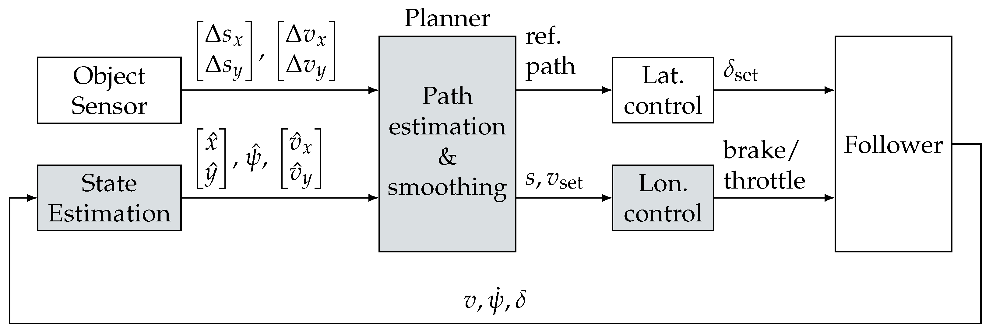
  • Unfortunately, the resulting spline from the spline-approximation algorithm, according to [19], lacks the local support property. That is, a variation of a single data point not only affects the related spline segment but all spline segments, if just a single point of the underlying approximation data changes. Considering that the spline Γ serves as the reference path for the path-tracking controller, as shown in Figure 1, this could result in jumps of the control reference and eventually of the control error every time the spline is updated. Although there are controllers that implement bumpless transfer functionality that could handle steps in the control reference to some extent [22], this is usually not the case; see, for example, the well known Stanley [23] and Pure-Pursuit [24] path-tracking controllers. Therefore, the iterative approach mentioned above was implemented, since it enables the extension of the spline path Γ by a spline segment γ i + 1 , while letting the segments γ 1 , , γ i be unaffected.
  • According to (7), the computational effort mainly depends on the number n of spline segments, considering k and l as fixed. Therefore, the computational effort can be reduced compared to calculating the spline Γ for all points p 1 , , p N during each iteration, depending on the actual values of ν and N.
  • These improvements are at the cost of only achieving continuous zeroth derivatives at the spline’s breaks. Simulation results showed that requesting higher order continuity at the breaks results in a spline approximation becoming unstable over time. During field tests, this disadvantage turned out to be neglectable.
This smoothing strategy is demonstrated in Figure 2 based on real-world measurement data, where the leader/follower convoy was driving from the top-right corner to the bottom-left corner of the graph.
The black dotted line shows the estimated path, according to Section 2.1, where each dot represents a position measurement obtained from a camera sensor. The red line shows the resulting spline consisting of four spline segments, where the segment’s terminal points are highlighted by dots. Although the spline is only G 0 continuous at the breaks, the overall smoothness is significantly improved in contrast to the estimated path.

2.3. Vehicle Control

From a control-design point of view and according to Figure 1, the lateral and longitudinal motion of the follower vehicle was considered to be decoupled. The corresponding controllers are presented in the following.

2.3.1. Lateral Control

The theoretical background of the lateral control component used in the context of the presented vehicle-following system was published in [22,25]. Since then, it was successfully applied to several practical implementations such as lane keeping [26]. Therefore, only the essence is recapitulated here.
Based on the linear single-track model [27] and a linearized and time-discretized path-tracking error model [25,26], a state-feedback control law
δ set = v ^ y ψ ˙ e lat e ψ χ k lat
is obtained via LQR design. The path-tracking error model, according to the classification introduced in [18], is as follows: The reference is located in the vehicle’s center of gravity, the look-ahead distance is along the vehicle heading, while the lateral error e lat and heading error e ψ , with respect to the reference path, are perpendicular to the vehicle heading. To account for a varying vehicle speed and a speed-dependant look-ahead distance, the feedback law (8) was gain scheduled and implemented using a look-up table. The dynamics of the demonstrator vehicle’s steering actuator were considered by a first-order transfer function [26], introducing one additional state χ .
The choice of the actual path-tracking controller was predetermined by the related error model, which should fit the problem statement. For the present application, the task is to follow the leader path as close as possible, to avoid cutting curves. As this requirement can only be fulfilled for a single point of a four-wheeled vehicle, a reasonable choice is the center of gravity along the vehicle’s longitudinal axis, in conjunction with zero look-ahead distance. Given this configuration, a vanishing control error would imply that the center of gravity perfectly tracks the reference path. Unfortunately, the look-ahead distance cannot be decreased arbitrarily as this also reduces the closed-loop phase margin [28] and can eventually lead to instability. The actual values used during deployment are given in Section 3.
It is also worth noting, that with the presented design, it would have been easily possible to replace the current controller with any other controller based on the same error model. A classification of path-tracking controllers from the literature, regarding their underlying error model, is given in Table 2 of [18].

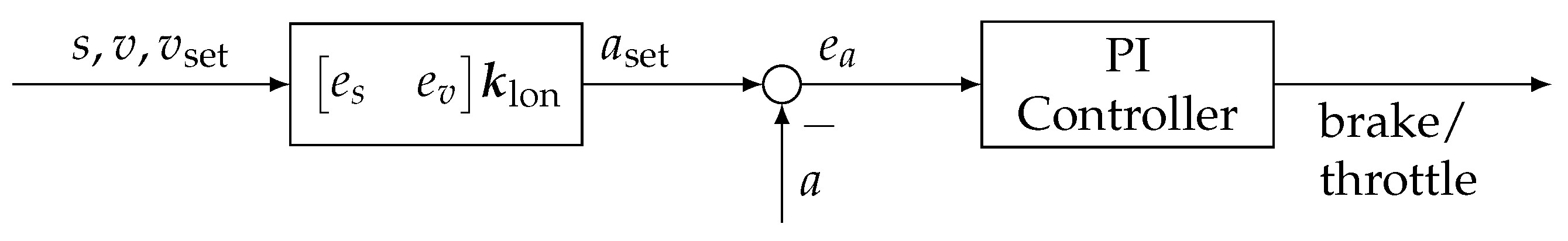
2.3.2. Longitudinal Control

The task of the longitudinal controller is to maintain a constant time gap t h from the leader vehicle, according to the constant time-headway policy [29]
s set = max { v set t h , s min }
given a desired speed v set and a minimum safety distance s min . The desired speed v set refers to the leader vehicle’s speed and was estimated according to
v set = v ^ x + v x ψ ˙ r sin ( θ ) v ^ y + v y + ψ ˙ r cos ( θ )
from on-board measurements, where
r = s x 2 + s y 2
θ = atan2 ( s y , s x )
are the distance r and bearing θ to the leader.
Considering that the distance s from the follower to the leader vehicle is negative, proportional with respect to the follower speed v, the follower’s longitudinal dynamics can be modeled as
x ˙ = 0 1 0 0 x + 0 1 a ,
with acceleration a and state x = [ s v ] t . The distance s to the leader is with respect to the reference path and determined via a Frenet transformation of the ego vehicle’s position. The error model then reads as
e = x set x
with distance error e s = s set s and velocity error e v = v set v . For the model (12), a controller
a set = k lon t e
can be designed via, e.g., pole placement.
The follower’s longitudinal-control strategy was eventually implemented as a cascaded control loop, according to Figure 3, where the desired acceleration (14) is tracked by the inner loop, implementing a PI controller.
This architecture was mainly motivated by the brake and throttle interfaces available in the test vehicle, in terms of pedal positions.

3. Test-Vehicle Integration and Field Trials

Until here, the vehicle-following system was mainly presented from a simulation-based perspective. This section discusses practical aspects related to the deployment of the proposed following system and also presents test results obtained under real operating conditions utilizing a series-production demonstrator car.

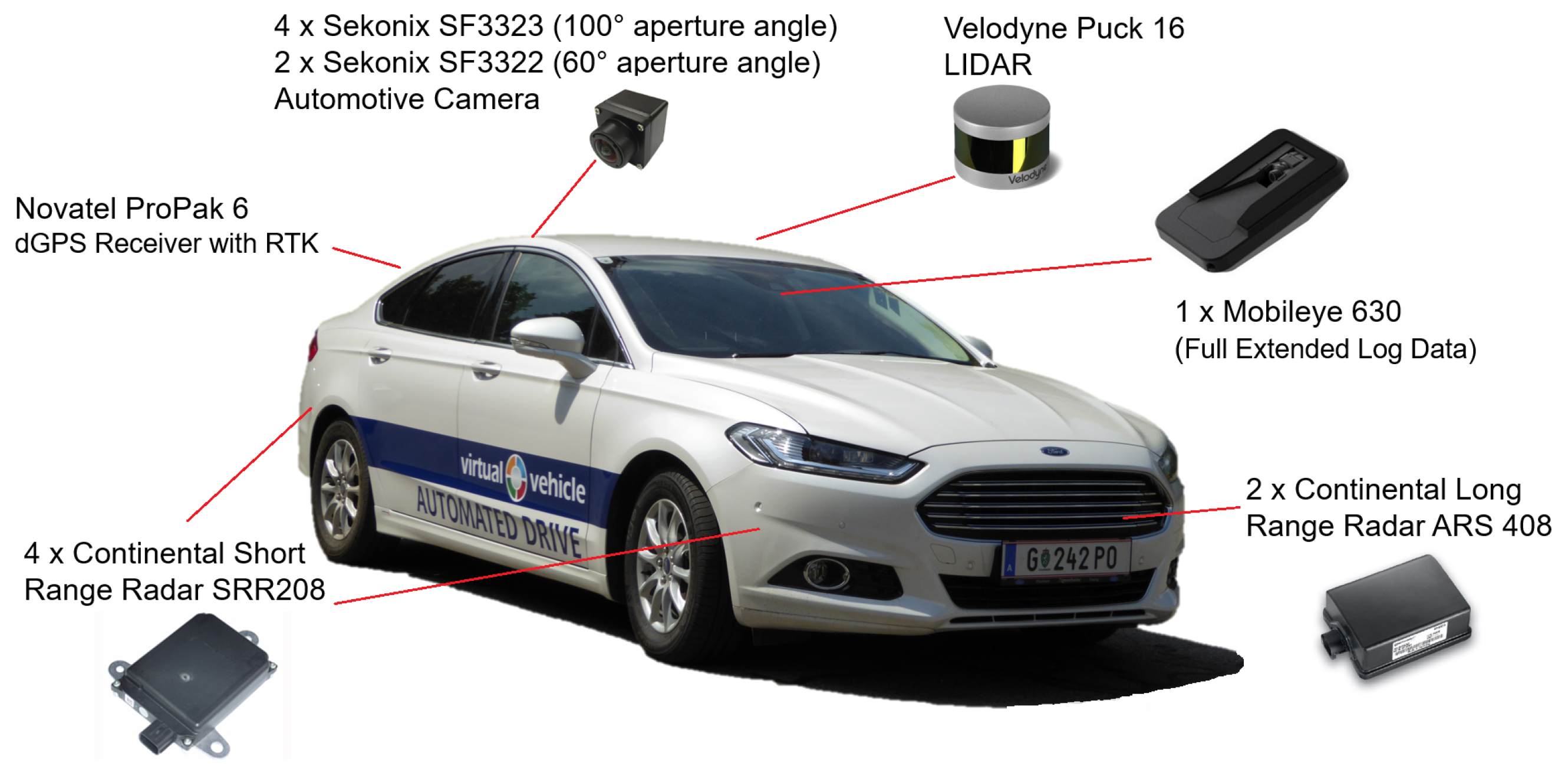
3.1. Demonstrator Vehicle

The demonstrator vehicle is a Ford Mondeo 2.0 Hybrid equipped with additional sensors and hardware; an overview is shown in Figure 4.
A so-called ADAS Kit from Dataspeed Inc. gives access to the vehicle’s CAN-bus. This allows for control of the steering wheel angle as well as brake and throttle via pedal-position commands. It also provides on-board sensor measurements like speed, acceleration, yaw rate, and series-production GPS readings.
The developed algorithms were deployed to a dSPACE MicroAutoBox II, equipped with a DS1401 processor board and 1511/1512 I/O boards. This setup served as the real-time control hardware executing the planning, state estimation, and vehicle-control algorithms. Additionally, RTMaps running on an industrial-grade PC was used as the interface to the Novatel differential GPS. This data was then transmitted to the MicroAutoBox via ethernet. Since the Mobileye 630 camera sensor provided the most robust object detection and classification, it was used during the field tests.

3.2. State Estimation

As pointed out in Section 2, estimates of the followers position ( x ^ , y ^ ) and orientation ψ ^ with respect to an inertial frame are required. This was accomplished by a dead-reckoning approach using a kinematic vehicle model [30] (p. 26)
x ^ ( t ) = 0 t v ( ξ ) cos ( β ^ ( ξ ) + ψ ^ ( ξ ) ) d ξ
y ^ ( t ) = 0 t v ( ξ ) sin ( β ^ ( ξ ) + ψ ^ ( ξ ) ) d ξ
ψ ^ ( t ) = 0 t ψ ˙ ( ξ ) d ξ
β ^ ( t ) = atan2 ( l r tan ( δ ( t ) ) , l f + l r ) .
In compliance with the requirements from Section 1.1, the implementation of (15) only requires measurements from on-board sensors, namely the vehicle speed v, the front-wheel steering angle δ , and the yaw rate ψ ˙ . Additionally, the front and rear axle offset from the center of gravity, denoted by l f and l r , are required.
Over time, this approach causes the estimates to deviate from the true position ( x , y ) and true orientation ψ . Assuming that the follower is tracking the leader vehicle with a steady-state time gap t h , the error between the actual and estimated values must be sufficiently small. In other words, the estimation error that accumulated during the time between obtaining a specific leader position until reaching this position is required to be small, to ensure satisfactory path tracking. This also implies that an upper bound for the time gap t h exists, depending on the estimation accuracy of the follower’s position and orientation.

3.3. Leader Selection

To simplify the development of the vehicle-following system, the task of identifying the leader vehicle from a list of multiple objects was neglected in simulations. Instead, just a single object was used as the leader vehicle. For the practical implementation during the field tests, object sensors mounted to the test vehicle were used for object detection. These sensors, like a camera, radar, or lidar, typically provide object lists containing not only the leader vehicle but also stationary objects or ghost objects. Therefore, a measure to identify the actual leader vehicle utilizing the spline path (5) was implemented.
From the path estimation and smoothing, an analytic formula of the leader path is available, given by the spline (5). Taking advantage of its analytic form, the path can easily be extrapolated by means of path parameter τ . For the actual implementation, the path parameter τ , referring to the arc length and the breaks τ 0 < τ 1 < < τ n , was obtained from the length of the polygonal path formed by the position measurements (2).
For the field tests, the actual path extrapolation distance was obtained by overestimating the traveled distance s of the leader vehicle, according to s = v set T s , where v set is the estimated leader speed (10) and T s is the sample time of the vehicle-following system. Given the extrapolated leader path and a list of objects, the leader vehicle was chosen as the closest object to the follower vehicle that intersects the extrapolated path. At initialization of the vehicle-following system, the estimated path is not available and the leader vehicle is selected according to the object type.

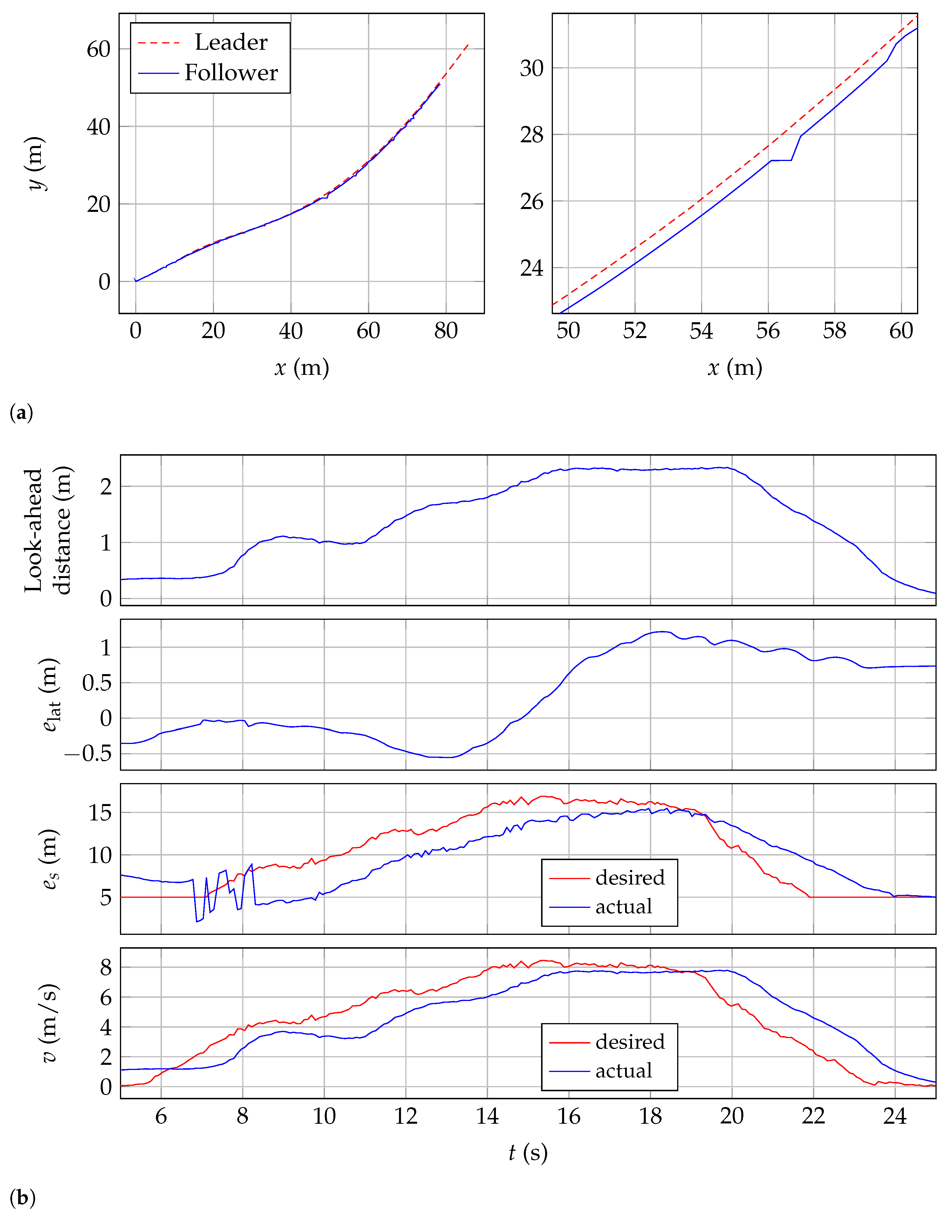
3.4. Experimental Results

The vehicle-following system was verified on a graveled land area at the campus of the Technical University of Graz, Austria. The tests were performed using two of Virtual Vehicle’s Automated Drive demonstrators; the automated follower vehicle is shown in Figure 4 and a bird’s-eye view of the test setup is shown in Figure 5.
Both the leader vehicle and the follower vehicle were equipped with DGPS to provide ground truth data. The vehicle-following system was executed on real-time hardware, as mentioned in Section 3.1, executing at a sample time of 20 m s . The complete list of parameters is stated in Table 1.
The test procedure was as follows: both vehicles were at a standstill, with the leader vehicle in front of the follower vehicle and within the object sensor’s field of view. After confirming leader detection, both vehicles started driving manually, meaning the follower vehicle needed to start idling before enabling the drive-by-wire mode.
Results of one exemplary trial are shown in Figure 6. Figure 6a shows a comparison of the leader and follower paths, while Figure 6b shows qualitative lateral and longitudinal control signals.
It should be pointed out, that the closed-loop lateral error e lat in Figure 6b is with respect to the reference path obtained from the spline-approximation algorithm. Since this path is an approximation of the estimated leader path, which is itself an estimate of the true leader path, the lateral error e lat does not reflect the follower’s offset from the true leader path. However, it reflects the performance of the path-tracking controller. According to the follower’s speed, the look-ahead distance varies during the trial. Although the related lateral-path tracking error e lat varies between roughly −0.5 m –1 m , the lateral offset with respect to the follower’s center of gravity stayed well between −0.4 m –0.4 m (Figure 6a). Around 7 s –8 s , the actual inter-vehicle distance s shows noisy characteristics. At this point in time, the follower reached the leader’s initial position, which was starting from a standstill. Due to that, several similar position measurements were added to the list (2), although the leader was not moving. This could have been avoided by tuning the area threshold parameter A ¯ with respect to the noise characteristics of the object sensor as well as the follower state estimation. Unfortunately, time constraints did not allow further investigation of this topic, as these effects are not easily reproducible during field trials. For future tests, recreating these effects in simulation to tune the related parameters beforehand is planned.

4. Conclusions and Outlook

In this work we have presented the concept, architecture, and real-world implementation of a state-of-the-art vehicle following a system relying on on-board sensors only. For detection of the leader vehicle, an optical sensor mounted to the follower vehicle was used. To obtain an estimate of the leader path, a new algorithm was proposed that considers the importance of new leader measurements with respect to the currently estimated path.
The smoothness of this estimated path was improved by a spline-approximation algorithm, which closes the gap between simple polynomial-fitting approaches [9] and computational-demanding ones, like presented in [10]. For the proof of concept of the proposed algorithms, field trials were performed on a graveled area achieving path-tracking errors between −0.4 m –0.4 m . We assume that these values can be improved by either tuning the existing path-tracking controller or implementing a more sophisticated one, which would be easily possible with the presented architecture.
For the future, it is planned to perform more extensive field trials utilizing various sensors for object detection. Another branch of investigation is regarding the path-tracking controller. The generic interface between the planning and the path-tracking component allows to benchmark various controllers from the literature and investigate the influence of their specific error models.

Author Contributions

Conceptualization, G.N. and J.R.; software, G.N.; validation, G.N.; writing—original draft preparation, G.N.; writing—review and editing, G.N., J.R. and S.S.; visualization, G.N.; supervision, G.N. All authors have read and agreed to the published version of the manuscript.

Funding

The publication was written at Virtual Vehicle Research GmbH in Graz, Austria. The authors would like to acknowledge the financial support within the COMET K2 Competence Centers for Excellent Technologies from the Austrian Federal Ministry for Climate Action (BMK), the Austrian Federal Ministry for Digital and Economic Affairs (BMDW), the Province of Styria (Dept. 12), and the Styrian Business Promotion Agency (SFG). The Austrian Research Promotion Agency (FFG) has been authorized for the program management.

Acknowledgments

The authors would like to express their thanks to the supporting industrial partner Infineon Austria.

Conflicts of Interest

The authors declare no conflict of interest.

Abbreviations

The following abbreviations are used in this manuscript:
CANController Area Network
DGPSDifferential Global Positioning System
GPSGlobal Positioning System
HDHigh Definition
LQRLinear Quadratic Regulator
MPCModel Predictive Control
PIProportional-Integral
SQPSequential Quadratic Programming
V2VVehicle-to-Vehicle

References

  1. On-Road Automated Driving (ORAD) Committee. Taxonomy and Definitions for Terms Related to Driving Automation Systems for On-Road Motor Vehicles; Technical Report; SAE International: Warrendale, PA, USA, 2021. [Google Scholar] [CrossRef]
  2. Zhang, L.; Ahamed, T.; Zhang, Y.; Gao, P.; Takigawa, T. Vision-Based Leader Vehicle Trajectory Tracking for Multiple Agricultural Vehicles. Sensors 2016, 16, 578. [Google Scholar] [CrossRef] [PubMed] [Green Version]
  3. Gehrig, S.K.; Stein, F.J. A trajectory-based approach for the lateral control of car following systems. SMC’98 Conference Proceedings. In Proceedings of the 1998 IEEE International Conference on Systems, Man, and Cybernetics (Cat. No.98CH36218), San Diego, CA, USA, 14 October 1998; IEEE: Piscataway, NJ, USA, 1998; Volume 4, pp. 3596–3601. [Google Scholar] [CrossRef]
  4. Daviet, P.; Parent, M. Longitudinal and lateral servoing of vehicles in a platoon. In Proceedings of the Conference on Intelligent Vehicles, Tokyo, Japan, 19–20 September 1996; IEEE: Piscataway, NJ, USA, 1996; pp. 41–46. [Google Scholar] [CrossRef]
  5. Goi, H.K.; Giesbrecht, J.L.; Barfoot, T.D.; Francis, B.A. Vision-Based Autonomous Convoying with Constant Time Delay. J. Field Robot. 2010, 27, 430–449. [Google Scholar] [CrossRef]
  6. Goi, H.K.; Barfoot, T.D.; Francis, B.A.; Giesbrecht, J.L. Vision-Based Vehicle Trajectory Following with Constant Time Delay. In Field and Service Robotics; Howard, A., Iagnemma, K., Kelly, A., Eds.; Springer: Berlin/Heidelberg, Germany, 2010; pp. 137–147. [Google Scholar] [CrossRef]
  7. Shan, M.; Zou, Y.; Guan, M.; Wen, C.; Lim, K.Y.; Ng, C.L.; Tan, P. Probabilistic trajectory estimation based leader following for multi-robot systems. In Proceedings of the 2016 14th International Conference on Control, Automation, Robotics and Vision (ICARCV), Phuket, Thailand, 13–15 November 2016; IEEE: Piscataway, NJ, USA, 2016; pp. 1–6. [Google Scholar] [CrossRef]
  8. Zou, Y.; Shan, M.; Guan, M.; Wen, C.; Lim, K.Y. A trajectory reconstruction approach for leader-following of multi-robot system. In Proceedings of the 2017 12th IEEE Conference on Industrial Electronics and Applications (ICIEA), Siem Reap, Cambodia, 18–20 June 2017; IEEE: Piscataway, NJ, USA, 2017; pp. 1534–1539. [Google Scholar] [CrossRef]
  9. Jansen, W.L. Lateral Path-Following Control of Automated Vehicle Platoons. Master’s Thesis, Delft University of Technology, Delft, The Netherlands, 2016. [Google Scholar]
  10. Fassbender, D.; Heinrich, B.C.; Luettel, T.; Wuensche, H.J. An optimization approach to trajectory generation for autonomous vehicle following. In Proceedings of the 2017 IEEE/RSJ International Conference on Intelligent Robots and Systems (IROS), Vancouver, BC, Canada, 24–28 September 2017. [Google Scholar] [CrossRef]
  11. Heald, M.A. Rational approximations for the Fresnel integrals. Math. Comput. 1985, 44, 459–461. [Google Scholar] [CrossRef]
  12. Wei, S.; Zou, Y.; Zhang, X.; Zhang, T.; Li, X. An Integrated Longitudinal and Lateral Vehicle Following Control System With Radar and Vehicle-to-Vehicle Communication. IEEE Trans. Veh. Technol. 2019, 68, 1116–1127. [Google Scholar] [CrossRef]
  13. Wang, Y.; Bian, N.; Zhang, L.; Chen, H. Coordinated Lateral and Longitudinal Vehicle-Following Control of Connected and Automated Vehicles Considering Nonlinear Dynamics. IEEE Control. Syst. Lett. 2020, 4, 1054–1059. [Google Scholar] [CrossRef]
  14. Floren, M.; Khajepour, A.; Hashemi, E. An Integrated Control Approach for the Combined Longitudinal and Lateral Vehicle Following Problem. In Proceedings of the 2021 American Control Conference (ACC), New Orleans, LA, USA, 25–28 May 2021; IEEE: Piscataway, NJ, USA, 2021; pp. 436–441. [Google Scholar] [CrossRef]
  15. Liu, J.; Wang, Z.; Zhang, L. Event-Triggered Vehicle-Following Control for Connected and Automated Vehicles under Nonideal Vehicle-to-Vehicle Communications. In Proceedings of the 2021 IEEE Intelligent Vehicles Symposium (IV), Nagoya, Japan, 11–17 July 2021; IEEE: Piscataway, NJ, USA, 2021; pp. 342–347. [Google Scholar] [CrossRef]
  16. Schinkel, W.; van der Sande, T.; Nijmeijer, H. State Estimation for Cooperative Lateral Vehicle Following Using Vehicle-to-Vehicle Communication. Electronics 2021, 10, 651. [Google Scholar] [CrossRef]
  17. Visvalingam, M.; Whyatt, J.D. Line generalisation by repeated elimination of points. Cartogr. J. 1993, 30, 46–51. [Google Scholar] [CrossRef]
  18. Rumetshofer, J.; Stolz, M.; Watzenig, D. A Generic Interface Enabling Combinations of State-of-the-Art Path Planning and Tracking Algorithms. Electronics 2021, 10, 788. [Google Scholar] [CrossRef]
  19. Ezhov, N.; Neitzel, F.; Petrovic, S. Spline approximation, Part 1: Basic methodology. J. Appl. Geod. 2018, 12, 139–155. [Google Scholar] [CrossRef]
  20. Eilers, P.H.C.; Marx, B.D. Flexible smoothing with B-splines and penalties. Stat. Sci. 1996, 11, 89–121. [Google Scholar] [CrossRef]
  21. Goepp, V.; Bouaziz, O.; Nuel, G. Spline Regression with Automatic Knot Selection. arXiv 2018, arXiv:1808.01770. [Google Scholar]
  22. Nestlinger, G.; Stolz, M. Bumpless Transfer for Convenient Lateral Car Control Handover. IFAC-PapersOnLine 2016, 49, 132–138, Special Issue: In Proceedings of the 9th IFAC Symposium on Intelligent Autonomous Vehicles IAV 2016, Leipzig, Germany, 29 June–1 July 2016. [Google Scholar] [CrossRef]
  23. Hoffmann, G.M.; Tomlin, C.J.; Montemerlo, M.; Thrun, S. Autonomous Automobile Trajectory Tracking for Off-Road Driving: Controller Design, Experimental Validation and Racing. In Proceedings of the 2007 American Control Conference, New York, NY, USA, 9–13 July 2007; IEEE: Piscataway, NJ, USA, 2007; pp. 2296–2301. [Google Scholar] [CrossRef]
  24. Coulter, R.C. Implementation of the Pure Pursuit Path Tracking Algorithm; Technical Report; Camegie Mellon University: Pittsburgh, PA, USA, 1992. [Google Scholar]
  25. Nestlinger, G. Modellbildung und Simulation Eines Spurhalte-Assistenzsystems. Master’s Thesis, Graz University of Technology, Graz, Austria, 2013. [Google Scholar]
  26. Solmaz, S.; Nestlinger, G.; Stettinger, G. Compensation of Sensor and Actuator Imperfections for Lane-Keeping Control Using a Kalman Filter Predictor. SAE Int. J. Connect. Autom. Veh. 2021, 4, 8. [Google Scholar] [CrossRef]
  27. Riekert, P.; Schunck, T. Zur Fahrmechanik des gummibereiften Kraftfahrzeugs. Ingenieur-Archiv 1940, 11, 210–224. [Google Scholar] [CrossRef]
  28. Hsu, J.C.; Tomizuka, M. Analyses of Vision-based Lateral Control for Automated Highway System. Veh. Syst. Dyn. 1998, 30, 345–373. [Google Scholar] [CrossRef]
  29. Swaroop, D.; Rajagopal, K. A review of constant time headway policy for automatic vehicle following. In Proceedings of the 2001 IEEE Intelligent Transportation Systems, Oakland, CA, USA, 25–29 August 2001; IEEE: Piscataway, NJ, USA, 2001; pp. 65–69. [Google Scholar] [CrossRef]
  30. Rajamani, R. Lateral Vehicle Dynamics. In Vehicle Dynamics and Control; Mechanical Engineering Series; Springer: New York, NY, USA, 2012; Chapter 2; pp. 15–46. [Google Scholar] [CrossRef]
Figure 1. System architecture of the developed vehicle-following system. Shaded components are addressed in this paper, while the main contribution is regarding the Planner component.
Electronics 11 01866 g001
Figure 2. Estimated path from sensor measurements and resulting spline path after applying the spline-approximation algorithm.
Electronics 11 01866 g002
Figure 3. Longitudinal dynamics control structure consisting of an outer control loop that regulates spacing error e s and speed error e v as well as an inner loop regulating acceleration error e a .
Electronics 11 01866 g003
Figure 4. Ford Mondeo demonstrator vehicle with additionally installed sensors. For the implementation presented in this paper, only the Mobileye 630 was used.
Electronics 11 01866 g004
Figure 5. Bird’s-eye view of the leader (left) and follower (right) vehicle setup, taken during the field tests. Video footage is available online at https://youtu.be/0EnHqTouIuc (Accessed on 1 May 2022).
Electronics 11 01866 g005
Figure 6. Results from an exemplary field trial run. (a) Leader and follower path obtained from differential GPS. The close-up (right figure) also shows an outlier around coordinate (57, 27). Due to its minor character and time constraints, we did not investigate the root cause. (b) Speed-dependent look-ahead distance, related lateral-tracking error, and longitudinal control signals in terms of distance and speed.
Electronics 11 01866 g006
Table 1. Parameter values used throughout the field trials.
NameSymbolValue
Sample time T s 20 m s
Max. number points N ¯ 100
Area threshold A ¯ 1 × 10 4   m 2
Min. clearance s min 5 m
Time gap t h 2 s
Look-ahead time300 m s
Samples per spline segment ν 12
Polynomial degreek3
Geometric continuityl2
Publisher’s Note: MDPI stays neutral with regard to jurisdictional claims in published maps and institutional affiliations.

