Deep Learning-Based End-to-End Carrier Signal Detection in Broadband Power Spectrum

Abstract

This paper presents an end-to-end deep convolutional neural network (CNN) model for carrier signal detection in the broadband power spectrum, so-called spectrum center net (SCN). By regarding the broadband power spectrum sequence as a one-dimensional (1D) image and each subcarrier on the broadband as the target object, we can transform the carrier signal detection problem into a semantic segmentation problem on a 1D image. Here, the core task of the carrier signal detection problem turns into the frequency center (FC) and bandwidth (BW) regression. We design the SCN to classify the broadband power spectrum as inputs and extract the features of different length scales by the ResNet backbone. Then, the feature pyramid network (FPN) neck fuses the features and outputs the fusion features. Next, the RegNet head regresses the power spectrum distribution (PSD) prediction for FC and the corresponding BW prediction. Finally, we can achieve the subcarrier targets by applying non-maximum suppressions (NMS). Moreover, we train the SCN on a simulation dataset and validate it on a real satellite broadband power spectrum set. As an improvement of the fully convolutional network-based (FCN-based) method, the proposed method directly outputs the detection results without post-processing. Extensive experimental results demonstrate that the proposed method can effectively detect the subcarrier signal in the broadband power spectrum as well as achieve higher and more robust performance than the deep FCN- and threshold-based methods.

1. Introduction

With the rapid development of wireless mobile communication, satellite communication, and other communication technologies, the electromagnetic spectrum space has become very complex and crowded. The safe use and effective control of the electromagnetic spectrum have turned into the critical task of radio monitoring, particularly in the non-cooperative electromagnetic spectrum monitoring field. Carrier signal detection is the first and most crucial step of non-cooperative signal processing. Through accurately detecting only the signal in the spectrum, we can further perform modulation recognition, channel coding identification, source coding identification, specific emitter identification, and other information analysis processes.

Few algorithms [1,2,3,4,5,6] are available for carrier signal detection, and these algorithms are mainly based on threshold values and human intervention, although some improvements have been noted using the double-thresholds method [7,8]. Kim et al. [9] proposed the use of a slope tracing-based algorithm to separate the interval of signal elements based on signal properties, such as amplitude, slope, deflection width or distance between neighboring deflections. For the practical application of these methods, many restrictions exist due to the fact that some parameters cannot be accurately estimated as well as the high complexity of computations.

Recently, artificial intelligence (AI), including machine learning, deep learning, and reinforcement learning, has been steadily growing as a research field and has shown successful results in diverse applications. Moreover, deep learning is one of the most exciting and fast-growing techniques with numerous improvements, particularly in domains, such as computer vision and natural language processing [10]. Meanwhile, many researchers have performed considerable exploration of AI and its application in wireless communication [11,12,13]. O’Shea et al. [14] discussed several deep learning applications for the physical layer. They introduced a new way of thinking about communications as an end-to-end reconstruction optimization task, using autoencoders to jointly learn transmitter and receiver implementations as well as signal encodings without prior knowledge.

Deep learning has been applied to carrier signal detection. For example, Morozov and Ovchinnikov [15] applied a fully connected neural network for the detection of FSK signals. Moreover, Li et al. [16] used generative adversarial network (GAN) and CNN for blind detection of underwater acoustic communication signals. In contrast, Yuan et al. [17] used deep learning for blind morse signal detection in wideband spectrum data.

Inspired by two-dimensional (2D) image semantic segmentation [18,19,20], we employed an FCN-based model [21] to solve the carrier signal detection problem in the broadband power spectrum. By regarding the broadband power spectrum sequence as a 1D image and each subcarrier on the broadband as the target object, we can transform the problem into a semantic 1D image segmentation problem. On the basis of the FCN-based model, the 1D deep CNN model was designed to categorize each point on a broadband power spectrum array into two categories (i.e., subcarrier or noise), then we can locate the subcarrier signals’ position on the broadband power spectrum. We use a simulated and real satellite broadband power spectrum dataset to train and validate the 1D CNN model, respectively. The experimental results demonstrate that the FCN-based method can successfully detect the subcarrier signal and achieve higher accuracy than the slope tracing method.

In accordance with [22], a deep learning-based framework named SigdetNet is applied to the multi-signal detection task, which focuses on each point classification of the power spectrum and is essentially based on FCN.

However, the FCN-based methods [21,22] cannot handle the carrier signal detection very well in these situations. One reason is that if a point in one subcarrier array has been categorized as noise, then the subcarrier would be wrongly recognized as two subcarriers. Another reason is that when two or more neighboring subcarriers are very close to each other, the FCN-based method cannot correctly distinguish between the demarcation points, and this would cause severe fault and leak detections.

In this paper, to solve the problems above, we propose SCN, an end-to-end CNN model based on deep learning. Contrary to the FCN-based method, which transforms the carrier signal detection problem into a semantic 1D segmentation image problem, we regard each subcarrier in the broadband power spectrum as an independent target object and directly localize its FC position and BW. Therefore, the carrier signal detection problem turns into a 1D image object localization problem. The proposed SCN classifies the broadband power spectrum as inputs and extracts the features of different length scales by the ResNet backbone. Then, the FPN [23] neck fuses the features and outputs the fusion features. Next, the RegNet head regresses the PSD prediction for FC and the corresponding BW prediction. Finally, we can achieve the subcarrier targets by applying NMS. Moreover, we train the SCN on a simulation dataset and evaluate it on an actual satellite broadband power spectrum set. As an improvement of the FCN-based method, the experimental results demonstrate that the proposed method can effectively detect the subcarrier signal in the broadband power spectrum as well as achieve higher and more robust performance than the FCN-based method. The main contributions of this work are summarized as follows:

• We propose an end-to-end deep CNN-based model for carrier signal detection in the broadband power spectrum, so-called SCN. Without prior knowledge and post-processing, the SCN directly achieves the detection results;
• We conducted several experiments to demonstrate the superiority of our proposed method compared with other existing methods. Additionally, the model scale and the amount of training simulation samples on the performance of the proposed method are investigated.

The remainder of this paper is organized as follows: Section 2 further describes the carrier signal detection problem in the broadband power spectrum. Section 3 introduces the details of the proposed method. Section 4 provides the specific experimentations, including the dataset for the experiments, training details, the evaluation results, and some comparisons with other methods. Finally, Section 5 concludes the paper.

2. Problem Description

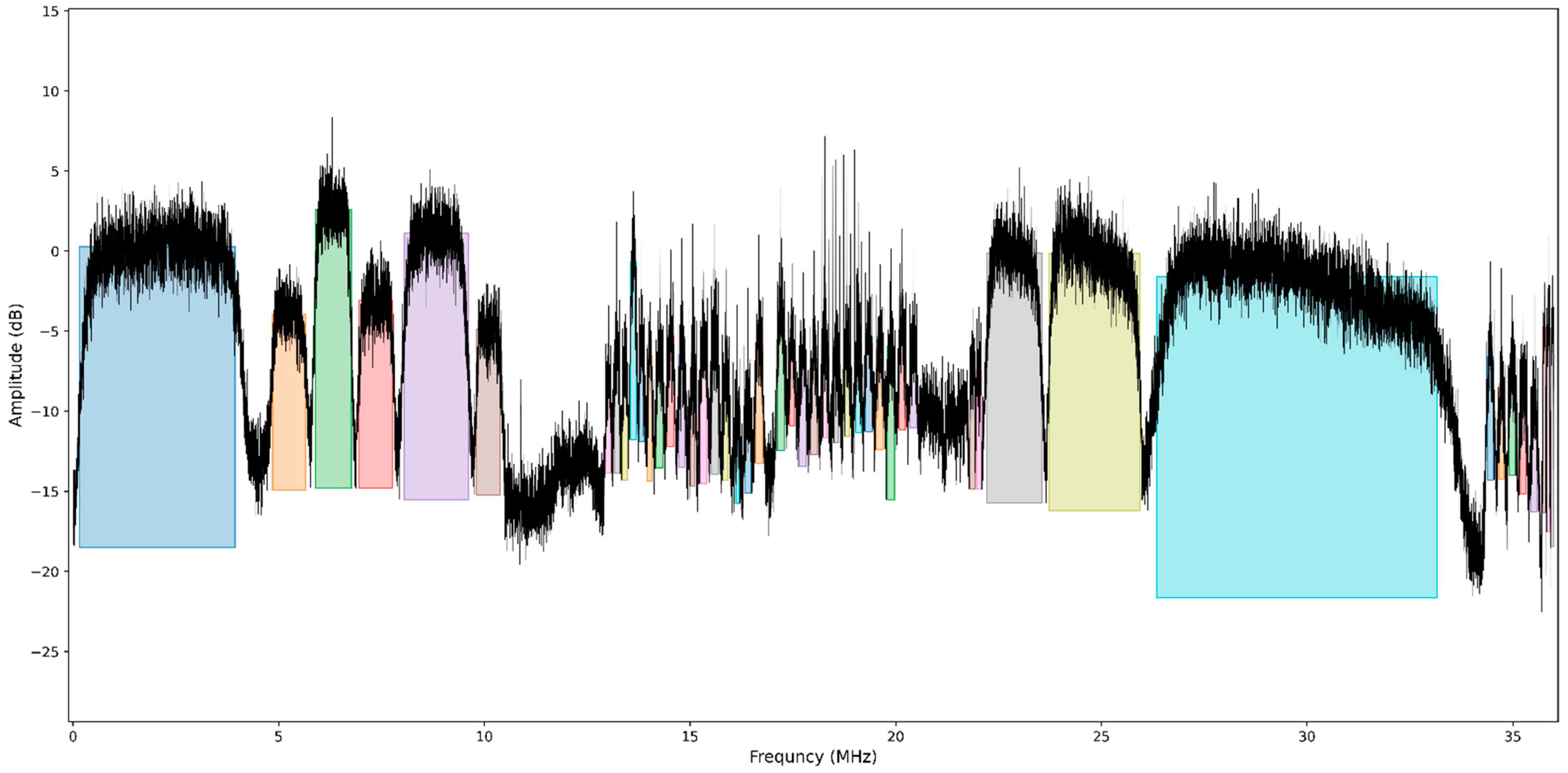
2.1. The Core Task of Carrier Signal Detection Problem

At present, in the 2D object detection problem, it is always preferrable to use a rectangle to localize the object in the images. Therefore, most of the end-to-end deep learning-based solutions are engaged in the regression of the corner points or center points position of the rectangle, as well as the width and height [24,25].

As Figure 1 shows, inspired by the 2D object detection problem, the 1D power spectrum is regarded as a 1D image and each subcarrier as an object. Moreover, we can use rectangles to localize the subcarriers. Therefore, the carrier signal detection problem turns into a 1D object localization problem. However, contrary to the 2D object detection problem, the core task of the carrier signal detection problem in the broadband power spectrum is the detection of the FC and BW of all subcarriers in the wideband power spectrum. Then, we can easily split the subcarrier signal from the broadband signal to perform modulation classification as well as further research and analysis.

The proposed SCN directly regresses the FC and BW in this paper and is an end-to-end carrier signal detector. Furthermore, its input is the broadband power spectrum, and the outputs are all of the subcarriers’ positions and the corresponding BW of the broadband.

2.2. The End-to-End Detection Process

Figure 2 shows the end-to-end detection process of the carrier signal detection in the broadband power spectrum. First, for the wideband time-domain signal, we utilize the Welch method [26,27] to estimate the broadband power spectrum. Then, considering that the broadband power spectrum is an input of the network, the proposed SCN can automatically regress the FC and the corresponding BW of all subcarriers.

The Welch power spectrum estimation is the average of the modified periodograms, namely:

$$P_{xx}^W=\frac{1}{k}{\displaystyle \sum }_{i=0}^{k-1}\frac{{\left|{{\displaystyle \sum }}_{n=0}^{M-1}{x}_i\left(n\right)\omega \left(n\right)e^{-j2\pi fn}\right|}^2}{{{\displaystyle \sum }}_{n=0}^{M-1}{\omega }^2\left(n\right)} i=0, 1, \dots ,k-1$$

(1)

The time-domain signal sequence is separated into k data segments with an overlap of 50% and a length of 2M. Additionally,$\omega \left(n\right)$ is the window function of a normalization factor for the power estimation results.

3. Methodology

3.1. SCN Architecture

Figure 3 presents the architecture of the SCN, which includes three main parts, the residual backbone, the FPN neck, and the RegNet head. The inputs of the SCN are the 1D broadband power spectrum, and the model outputs are PSD and BW regressions. Moreover, all the local maximums of PSD regression are the subcarrier FC positions.

• The Residual backbone

The residual backbone in SCN is modified by the deep residual network (ResNet) [28], which is widely used in the computer vision field. Additionally, it has emerged as a family of extremely deep architectures showing compelling accuracy and excellent convergence behaviors. In our work, since the inputs are a batch of 1D broadband power spectrum sequences, all of the parameters are suitable for setting the dimension of the inputs. Meanwhile, we still utilize the 2D Conv application interface (API) and fix the features to the width channel. For instance, if the Conv kernel size is $\left(1,k\right)$ with a stride of $\left(1,s\right)$, then the padding size would be $\left(1,\left(k-1\right)/\left(2\times s\right)\right)$.

As can be seen in Figure 3, we add a convolutional block attention module (CBAM) [29] for better feature extraction prior to the residual blocks. Contrary to the original CBAM, we directly concatenate the average global pooling (GAP) and maximum global pooling (GMP) features in the channel attention module (CAM). Additionally, we use a 1 × 1 Conv to replace the shared multilayer perceptron (MLP). Moreover, we set the groups to four to reduce the computing complexity.

In Figure 3, the residual layer in SCN is contrary to the original residual layer. Herein, we add a simplified CAM (S-CAM) prior to the last non-linear activation of the residual layer. Compared with the CAM, only GAP is used prior to the 1 × 1 Conv in S-CAM. Additionally, we use only one residual block and downsample the feature length in each residual layer, thus the downscale increases by two times. In our work, the input spectrum length is set to 32,768, which is considerably longer than the 2D image size in the object detection tasks. Therefore, we can set the downsample times (M) between 6 to 13 and name the whole corresponding model as SCN-M×. In the architecture of SCN-13× and the residual backbone, the number in the boxes represents the strides to the input spectrum length, which increases with the number of residual layers and is equal to $2^M$, as shown in Figure 3. Moreover, the output features of each residual layer are called PM. Furthermore, to reduce the complexity of the original residual layers, the number of feature maps is set to $64+32 M$.

• The FPN Neck

Feature pyramid structures (FPN) are essential in recognition systems to detect objects at different scales [23]. This top-down architecture builds high-level semantic feature maps with lateral connections at all scales. We utilize FPN as the features fusion neck module, as shown in Figure 3. With the skip-connections, the inputs of FPN are the outputs of the residual layers. We use the bilinear mode in the upsample layers and perform the last regression at four strides to the input spectrum length. All the Conv layers in the FPN head contain 256 channels. This architecture efficiently fuses all the top-to-bottom scale features.

• The Regression Network Head

The PSD and BW regressions are produced by almost the same structure modules in the RegNet head, as shown in Figure 3. The modules consist of a depthwise separable convolutional layer [30] with 256 channels, rectified linear unit (ReLU) [31], and a 1 × 1 Conv with one channel in common. However, we hope that in the PSD regression, all the values in the subcarrier center position are 1 and the others are considered as background and 0. Therefore, we can use the non-linear sigmoid function as the output layer. Moreover, since we directly regress the BW, the ReLU is used for the BW regression output layer to ensure positive results.

3.2. SCN Training Targets and Loss Function

As mentioned above, in SCN, we regress the two sets of prediction key points, PSD prediction for subcarrier FC positions and the corresponding BW prediction.

In Figure 4, the PSD targets are an example of the input power spectrum. Let $I\in S^L$ be an input power spectrum of length $L$. Therefore, we aim to produce the PSD outputs $P\in {\left[0, 1\right]}^{\frac{L}{4}}$ for the set output stride to a fixed value of 4 in SCN. Let $P_i$ be the score at the $i_{th}$ point in the predicted PSD, and let $Y_i$ be the ground-truth PSD, where the subcarrier center denotes $P_i=1$, corresponding to a detected keypoint, while the others are all background and $P_i=0$. In accordance with [24,25], a 1D Gaussian kernel $e^{-\frac{{\left(x-P_x\right)}^2}{2{\sigma }^2}}$ is used to produce the ground-truth at the frequency center of the PSD, where $\sigma$ is 1/3 of the corresponding BW. If the two Gaussians overlap, we consider the element-wise maximum [32].

In the training phase, we utilize a modified focal loss [33] to optimize the PSD outputs:

$$L_{psd}=-\frac{1}{N}{\displaystyle \sum }_{i=1}^L\{\begin{array}{c}{\left(1-P_i\right)}^{\alpha }\log \left(P_i\right) if Y_i=1\\ {\left(1-Y_i\right)}^{\beta }{\left(P_i\right)}^{\alpha }\log \left(1-P_i\right) otherwise\end{array}$$

(2)

where $\alpha$ and $\beta$ are hyper-parameters of the modified focal loss and $N$ is the number of all subcarriers in the power spectrum. We set $\alpha$ to 2 and $\beta$ to 4 in all our experiments. The loss reduces the penalty around the ground-truth locations.

Let $BSW$ be the broadband power spectrum bandwidth, and let $B{W}^k$ be the $k_{th}$ subcarrier bandwidth. Therefore, we can use an embedding vector to predict the BW regression. Here, the $k_{th}$ subcarrier center is the ground-truth embedding value set to ${\widehat{W}}^k=\frac{L\times B{W}^k}{BSW}$. As a result, we can predict a set of BW regression embedding and directly use the raw spectrum coordinates without normalizing the scale, so-called $W^k$. To train the BW regression, we utilize a L1 loss at the center point of the subcarrier. All the other locations are not considered and the formula is as follows:

$$L_{bw}=-\frac{1}{N}{\displaystyle \sum }_{k=1}^N\left|{\widehat{W}}^k-W^k\right|$$

(3)

To balance the PSD and BW losses, we use a constant ${\lambda }_{bw}$ to scale the BW loss. The overall training loss is as follows:

$$L_{det}=L_{psd}+{\lambda }_{bw}{L}_{bw}$$

(4)

In all our experiments, ${\lambda }_{bw}=0.1$.

3.3. SCN Inference Details

The aim of this work is to utilize SCN for the detection of the carrier signal results directly with the fusion of PSD and BW regressions in the inference phase.

First, we apply a 1 × 7 max pooling layer on the PSD regression to avoid the local maximum at inference time. Then, we pick the top 300 centers from the PSD regression, which are the scores of the predicted subcarriers. As a result, we can achieve the predicted subcarriers with the corresponding BW prediction by applying NMS.

In the NMS process, the intersection-over-unit (IoU) on carriers is defined by the following formula:

$$Io{U}_{carrier}=\frac{B{W}_{overlap}}{B{W}_{union}}$$

(5)

where the $B{W}_{overlap}$ and $B{W}_{union}$ are the length of overlap and length of union between the two predicted subcarriers, as shown in Figure 5. The predicted subcarrier scores remain as > 0.7 and IoU > 0.9.

4. Experiments

4.1. Data Preparation

In accordance with [21], the test set is a set of real-world satellite broadband power spectrum, consisting of 9581 subcarriers whose carrier-to-noise ratio (CNR) are all greater than 4 dB and BW regressions are greater than 10 kHz. The satellite power spectrum bandwidth is 36 MHz, and the raw coordinate length is 32,768.

The training set produced by the MATLAB simulation signal power spectra is estimated by the Welch method with a simulation of complex time-domain signals. This produces 100,000 simulation samples for training the network. Additionally, in all the training processes, the ratio of the number of training sets between the validation sets is 4:1.

4.2. Model Training

As can be seen in

Table 1. SCN training parameters.

Implement Library	PyTorch 1.10.0
Hardware Platform	2 GeForce RTX 3080Ti GPU, Intel(R) Bronze 3204 CPU
Operation System	Ubuntu 20.04
Model Input Length	32,768
Batch Size	32
Training Epochs	150
Dropout Probability	0.3
Optimizer	Adam
Learning Rate Strategy	Cosine Annealing Warm Restarts, initial value 2 × 105, T_0 = 10, T_mult = 2

, we implement the SCN in PyTorch [34]. Additionally, the parameters of the network are randomly initialized under the default setting of PyTorch with no pre-training on any external dataset. During the training process, we set the input length of the network to 32,768, which leads to an output length of 8192. Moreover, we adopt Dropout [35] prior to RegNet to reduce overfitting.

Adam optimization method [36] is utilized to optimize the overall training loss. Moreover, we employ a batch size of 32 and the network on 2 NVidia GeForce RTX 3080Ti graphic process units (GPUs) (Santa Clara, CA, USA) and Intel(R) Bronze 3204 CPU (Santa Clara, CA, USA), Ubuntu 20.04 operation system (London, UK). Furthermore, all the models for 150 epochs are trained with a learning rate strategy of cosine annealing warm restarts [37].

This paper proposes two different methods to train the proposed SCN. The first method compares the different residual downsample layers with the same training simulation samples, while the second method compares the different numbers of training simulation samples with the same residual downsample layers, as shown in Figure 6 and Figure 7, respectively. In Figure 6, 20,000 simulation samples are used to train the networks. The residual downsample layer ranges from 6 to 13 and the results demonstrate that both the PSD and BW losses converge with the training epoch. Subsequently, they increase and decrease with the increasing number of residual downsample layers. In Figure 7, a total of 10,000, 20,000, 40,000, 60,000, 80,000, and 100,000 simulation samples are used to train SCN-11x. Moreover, the results demonstrate that both PSD and BW losses converge with the training epoch. Subsequently, they increase and decrease with the increasing number of training simulation samples. Nevertheless, the specific converged loss values indicate that the scale of residual downsample layers significantly influences the scale of training samples.

4.3. Evaluation Results

During the evaluation, we calculate the F-score by the average precision rate (AP) and average recall rate (AR) to quantify and compare the performance of different trained models using the following formula:

$$AP=\frac{{\displaystyle \sum }TP}{{\displaystyle \sum }TP+{\displaystyle \sum }TN}$$

(6)

$$AR=\frac{{\displaystyle \sum }TP}{{\displaystyle \sum }TP+{\displaystyle \sum }FN}$$

(7)

$$F\text{-}Score=\frac{2\ast AP\ast AR}{AP+AR}$$

(8)

where $TP$ (true positive) denotes the number of subcarriers that are correctly detected, $TN$(true negative) denotes the number of subcarriers that are wrongly detected, and $FN$ (false negative) denotes the number of subcarriers that are not detected, but are included in the test set. F-score is the harmonic means of $AP$ and $AR$ and is more reasonable than the arithmetic means [38].

Figure A1, Figure A2, Figure A3, Figure A4, Figure A5, Figure A6, Figure A7 and Figure A8 show qualitative examples of the actual satellite broadband power spectrum set. All the subcarriers in these broadband power spectra have been correctly located and colored with a rectangle, which indicates that the proposed method is effective and achieves outstanding performance.

• SCN Model scale influence

With the application of CNN-based deep learning method in many fields, several studies [28,39,40,41] show that the network scale (depth or layers) is significant for the performance of CNN. Moreover, the more layers used, the better the performance of the model. Furthermore, the different scales of SCN are validated on the test set with the number of residual layers ranging from 6 to 13.

In Figure 8a, the F-score increases with the SCN model scale. Moreover, Figure 8b shows the precision-recall (PR) curves of these SCNs. Both AR and AP achieve high area under the curve (AUC) values when the network scale is beyond SCN-8x. The SCN-6x and SCN-7x do not have a good recall ratio, which leads to a deployment problem in real applications. The results indicate that the proposed method is effective and accurate.

• The effect comparison of the training set amounts

At present, deep learning is a data-driven science [10]. The more training samples used, the better the model would perform to a certain extent. Figure 9 shows the evaluation results of the SCN-11x trained with different numbers of training sets. We can see that the performance increases slightly as the training samples increase. On the basis of our analysis, all of the training samples are generated randomly through simulation, thus the diversity of the samples is insufficient. However, this also indicates that we do not have to use plenty of training samples to train the network for carrier signal detection in the broadband power spectrum. Furthermore, the fewer training samples used, the lower the cost of training time.

• Complexity comparison

On the basis of the performance comparison of the SCN scale, we know that the model performs better with the SCN model scale. In comparison, the model complexity would also increase, as shown in

Table 2. The performance comparison between the proposed method and other methods.

	AP	AR	F-Score
Double-Thresholds	77.64%	68.21%	72.62%
Slope Tracing	89.18%	88.63%	88.90%
SigdetNet with DiceLoss	95.64%	98.82%	97.20%
SigdetNet with FocalLoss	98.01%	98.79%	98.40%
FCN-Based 1	90.29%	89.47%	89.88%
FCN-Based 2	92.56%	93.71%	93.13%
FCN-Based 3	93.09%	93.88%	93.48%
FCN-Based 4	94.62%	95.66%	95.14%
FCN-Based 5	95.65%	97.39%	96.51%
FCN-Based 6	97.89%	97.49%	97.69%
FCN-Based 7	98.32%	98.13%	98.22%
FCN-Based 8	98.30%	97.43%	97.86%
FCN-Based 9	98.23%	97.66%	97.94%
FCN-Based 10	98.26%	97.56%	97.91%
FCN-Based 11	98.20%	97.25%	97.72%
FCN-Based 12	98.10%	97.70%	97.90%
FCN-Based 13	98.26%	97.89%	98.07%
SCN-6×	98.35%	43.09%	59.93%
SCN-7×	99.27%	60.59%	75.25%
SCN-8×	99.70%	82.01%	89.99%
SCN-9×	99.75%	94.55%	97.08%
SCN-10×	99.45%	96.99%	98.21%
SCN-11×	99.84%	99.12%	99.48%
SCN-12×	99.73%	98.59%	99.15%
SCN-13×	99.88%	99.08%	99.48%

. In practice, real-time is an essential factor in signal processing. A more complex model increases the processing time. Therefore, we need the most efficient model to balance the performance and processing time cost. Additionally, as can be seen in Table 2, the performance of SCN-11× is as good as SCN-13×, but the inference time cost is 89.35% of SCN-13×, which is the most appropriate candidate.

4.4. Performance Comparison to Other Methods

To demonstrate the superiority of the SCN, the performance comparison is carried out with four other methods, including the double-thresholds method [7], the slope tracing method [9], the FCN-based models [21], and SigdetNet [22]. Both of these methods are evaluated on the same test datasets. The two deep learning-based methods (FCN-based models and SigdetNet) are trained with 20,000 simulation samples, as mentioned in Section 4.2.

Table 2 shows the performance comparison between the SCN method and other methods. Compared with the double-thresholds method and slope tracing method, both of the deep learning-based methods are significantly superior. From our analysis, setting the appropriate thresholds for these threshold-based methods is difficult, which is the main reason for the vast performance gaps from the deep learning-based methods.

Compared with SigdetNet, the deep learning method provides different results [22], while we found that FocalLoss performs better than DiceLoss in our experiments. However, the proposed SCN achieves better performance when the SCN scale is greater than 10.

As an improvement of the FCN-based method, the SCN method improves the AP from 98.32% to 99.88%, AR from 98.13% to 99.12%, and F-score from 98.22% to 99.48%, respectively. It is evident that the proposed method achieves higher AP scores than the FCN-based method at all different scales of networks. However, the higher AP scores scarify the AR scores when the scale of the network is small in the SCN method.

Table 3. The complexity comparison between the proposed method and the other deep learning-based methods.

	Time Cost/ms	FLOPs/M	Parameters/K
SigdetNet with FocalLoss	15.32	909.97	297.52
FCN-Based 1	2.01	6.29	16.03
FCN-Based 2	3.32	7.86	25.44
FCN-Based 3	3.49	8.65	34.85
FCN-Based 4	4.78	9.04	44.26
FCN-Based 5	5.24	9.24	53.66
FCN-Based 6	5.71	9.34	63.07
FCN-Based 7	6.14	9.39	72.48
FCN-Based 8	6.46	9.41	81.89
FCN-Based 9	7.23	9.42	91.3
FCN-Based 10	7.93	9.43	100.7
FCN-Based 11	9.11	9.43	110.11
FCN-Based 12	9.71	9.44	119.52
FCN-Based 13	12.28	9.44	128.93
SCN-6×	8.98	12,923.99	3312.23
SCN-7×	10.25	13,338.22	4120.42
SCN-8×	11.45	13,545.35	4928.61
SCN-9×	12.85	13,648.92	5736.8
SCN-10×	14.36	13,700.71	6544.99
SCN-11×	16.7	13,726.62	7353.19
SCN-12×	16.83	13,739.58	8161.38
SCN-13×	18.69	13,746.07	8969.57

shows the complexity comparison between SCN and the other deep learning-based methods. Although the floating-point operations (FLOPs) and network parameters of the SCN models are dozens of times more than the SigdetNet and FCN-based methods, the inference time cost only increases by 22.0% and 52.2%. Due to the fact that the proposed SCN method is an end-to-end deep learning-based network without post-processing, while the FCN-based and SigdetNet methods only predict the classification probability of each point of the inputs, they cannot directly achieve the detection results. Therefore, without the post-processing time cost, the proposed method achieves higher performance using a considerably more complex CNN-based model.

Furthermore, the SCN method prevents the typical problem and false detection of the FCN-based method, which successfully improves the detection performance. For example, Figure A4 shows that the SCN method locates the precise subcarrier, whose bandwidth is very wide and the power distribution is relatively uneven, while it is a typical example of false detection in FCN-based method.

5. Discussion and Conclusions

In this paper, an end-to-end deep learning-based method for carrier signal detection in the broadband power spectrum, so-called SCN, was proposed. By regarding the carrier signal problem as an object localization task in the 1D broadband power spectrum image rather than the segmentation task in the FCN-based method, the core task is to regress the centers of all subcarriers and their corresponding bandwidths. To improve the FCN-based method, we apply the attention mechanism and use more complex residual layers in the feature extraction modules. Then, the FPN neck fused the different scales of features and automated regressions to PSD and BW predictions by the RegNet head. As shown in Table 2, the experiments have suggested that the SCN method, through training with the simulation samples, effectively handles the carrier signal detection problem and achieves higher performance than the FCN- and threshold-based methods.

Moreover, in the training process, Figure 6 and Figure 7 suggest that the proposed model converges with the training epochs. Meanwhile, increasing the scale of the model or using more numbers of training samples both improve the PSD and BW loss to a lower value. However, while the SCN scale is beyond 8, the distance of performance on the validation simulation samples becomes smaller as the training epochs increase, as shown in Figure 8. Furthermore, in Figure 9, the number of training samples slightly impacts the validation performance when the losses converge. Considering that the validation samples are simulated in the same conditions as the training samples, our analysis indicates that the model tends to overfit as the losses converge. Increasing the variety of sample generation conditions or the actual signal sample numbers would help alleviate this phenomenon.

Finally, in the evaluation phase, the performance increases with the SCN scale, as shown in Table 2. Meanwhile, Table 3 indicates that the SCN method requires significant computation complexity, which causes more inference time than the FCN-based methods, even though the SCN methods do not require post-processing. Therefore, in our future work, we plan to reduce the computation complexity of the proposed method to allow for more efficiency in real applications.

References

1. Henttu, P.; Aromaa, S. Consecutive mean excision algorithm. In Proceedings of the IEEE Seventh International Symposium on Spread Spectrum Techniques and Applications, Prague, Czech Republic, 2–5 September 2002; Volume 2, pp. 450–454. [Google Scholar]
2. Saarnisaari, H. Consecutive mean excision algorithms in narrowband or short time interference mitigation. In Proceedings of the PLANS 2004. Position Location and Navigation Symposium (IEEE Cat. No.04CH37556), Monterey, CA, USA, 26–29 April 2004; pp. 447–454. [Google Scholar]
3. Escbbach, R.; Fan, Z.; Knox, K.T.; Marcu, G. Threshold modulation and stability in error diffusion. IEEE Signal Process. Mag. 2003, 20, 39–50. [Google Scholar] [CrossRef]
4. Saarnisaari, H.; Henttu, P. Impulse detection and rejection methods for radio systems. In Proceedings of the IEEE Military Communications Conference, 2003. MILCOM 2003, Boston, MA, USA, 13–16 October 2003; Volume 2, pp. 1126–1131. [Google Scholar]
5. Keane, H.G. A new approach to frequency line tracking. In Proceedings of the 1991 Conference Record of the Twenty-Fifth Asilomar Conference on Signals, Systems & Computers ACSSC, Pacific Grove, CA, USA, 4–6 November 1991; Volume 2, pp. 808–812. [Google Scholar]
6. Mustafa, H.; Doroslovacki, M.; Deng, H. Algorithms for emitter detection based on the shape of power spectrum. In Proceedings of the Conference on Information Sciences and Systems CISS, The Johns Hopkins University, Baltimore, MD, USA, 12–14 March 2003; pp. 808–812. [Google Scholar]
7. Vartiainen, J.; Lehtomaki, J.J.; Saarnisaari, H. Double-threshold based narrowband signal extraction. In Proceedings of the 2005 IEEE 61st Vehicular Technology Conference VTC, Stockholm, Sweden, 30 May–1 June 2005; Volume 2, pp. 1288–1292. [Google Scholar]
8. Vartiainen, J. Localization of multiple narrowband signals based on the FCME algorithm. In Proceedings of the Nordic Radio Symposium NRS, Oulu, Finland, 16–18 August 2004; Volume 1, p. 5. [Google Scholar]
9. Kim, J.; Kim, M.; Won, I.; Yang, S.; Lee, K.; Huh, W. A biomedical signal segmentation algorithm for event detection based on slope tracing. In Proceedings of the 2009 Annual International Conference of the IEEE Engineering in Medicine and Biology Society, Minneapolis, MN, USA, 3–6 September 2009; pp. 1889–1892. [Google Scholar]
10. LeCun, Y.; Bengio, Y.; Hinton, G. Deep learning. Nature 2015, 521, 436–444. [Google Scholar] [CrossRef] [PubMed]
11. Simeone, O. A Very Brief Introduction to Machine Learning with Applications to Communication Systems. IEEE Trans. Cogn. Commun. Netw. 2018, 4, 648–664. [Google Scholar] [CrossRef] [Green Version]
12. Chen, M.; Challita, U.; Saad, W.; Yin, C.; Debbah, M. Artificial Neural Networks-Based Machine Learning for Wireless Networks: A Tutorial. IEEE Commun. Surv. Tutor. 2019, 21, 3039–3071. [Google Scholar] [CrossRef] [Green Version]
13. Luong, N.C.; Hoang, D.T.; Gong, S.; Niyato, D.; Wang, P.; Liang, Y.-C.; Kim, D.I. Applications of Deep Reinforcement Learning in Communications and Networking: A Survey. IEEE Commun. Surv. Tutor. 2019, 21, 3133–3174. [Google Scholar] [CrossRef] [Green Version]
14. O’Shea, T.; Hoydis, J. An Introduction to Deep Learning for the Physical Layer. IEEE Trans. Cogn. Commun. Netw. 2017, 3, 563–575. [Google Scholar] [CrossRef] [Green Version]
15. Morozov, O.A.; Ovchinnikov, P.E. Neural Network Detection of MSK Signals. In Proceedings of the 2009 IEEE 13th Digital Signal Processing Workshop and 5th IEEE Signal Processing Education Workshop, Marco Island, FL, USA, 4–7 January 2009; pp. 594–596. [Google Scholar]
16. Li, Y.; Wang, B.; Shao, G.; Shao, S.; Pei, X. Blind Detection of Underwater Acoustic Communication Signals Based on Deep Learning. IEEE Access 2020, 8, 204114–204131. [Google Scholar] [CrossRef]
17. Yuan, Y.; Sun, Z.; Wei, Z.; Jia, K. DeepMorse: A Deep Convolutional Learning Method for Blind Morse Signal Detection in Wideband Wireless Spectrum. IEEE Access 2019, 7, 80577–80587. [Google Scholar] [CrossRef]
18. Ronneberger, O.; Fischer, P.; Brox, T. U-Net: Convolutional Networks for Biomedical Image Segmentation. In Medical Image Computing and Computer-Assisted Intervention; Springer: Munich, Germany, 2015; Volume 9351, pp. 234–241. [Google Scholar]
19. Shelhamer, E.; Long, J.; Darrell, T. Fully Convolutional Networks for Semantic Segmentation. IEEE Trans. Pattern Anal. Mach. Intell. 2017, 39, 640–651. [Google Scholar] [CrossRef] [PubMed]
20. He, K.; Gkioxari, G.; Dollár, P.; Girshick, R. Mask R-CNN. In Proceedings of the IEEE International Conference on Computer Vision (ICCV), Venice, Italy, 22–29 October 2017; pp. 2980–2988. [Google Scholar]
21. Huang, H.; Li, J.Q.; Wang, J.; Wang, H. FCN-Based Carrier Signal Detection in Broadband Power Spectrum. IEEE Access 2020, 8, 113042–113051. [Google Scholar] [CrossRef]
22. Lin, M.; Zhang, X.; Tian, Y.; Huang, Y. Multi-Signal Detection Framework: A Deep Learning Based Carrier Frequency and Bandwidth Estimation. Sensors 2022, 22, 3909. [Google Scholar] [CrossRef] [PubMed]
23. Lin, T.Y.; Dollár, P.; Girshick, R.; He, K.; Hariharan, B.; Belongie, S. Feature Pyramid Networks for Object Detection. In Proceedings of the 30th IEEE Conference on Computer Vision and Pattern Recognition, CVPR 2017, Honolulu, HI, USA, 21–26 July 2017; pp. 936–944. [Google Scholar]
24. Law, H.; Deng, J. Cornernet: Detecting objects as paired keypoints. In Proceedings of the 15th European Conference on Computer Vision (ECCV), Munich, Germany, 8–14 September 2018; pp. 734–750. [Google Scholar]
25. Zhou, X.; Wang, D.; Krähenbühl, P. Objects as points. arXiv 2019, arXiv:1904.07850. [Google Scholar]
26. Proakis, J.G.; Manolakis, D.G. Digital Signal Processing: Principles, Algorithms and Applications, 3rd ed.; Prentice-Hall: Hoboken, NJ, USA, 1996; pp. 910–913. [Google Scholar]
27. Welch, P. The use of fast Fourier transform for the estimation of power spectra: A method based on time averaging over short, modified periodograms. IEEE Trans. Audio Electroacoust. 1967, 15, 70–73. [Google Scholar] [CrossRef] [Green Version]
28. He, K.M.; Zhang, X.Y.; Ren, S.Q.; Sun, J. Deep Residual Learning for Image Recognition. In Proceedings of the IEEE Conference on Computer Vision and Pattern Recognition (CVPR), Seattle, WA, USA, 26 June–1 July 2016; pp. 770–778. [Google Scholar]
29. Woo, S.H.; Park, J.; Lee, J.Y.; Kweon, I.S. CBAM: Convolutional Block Attention Module. In Proceedings of the 15th European Conference on Computer Vision (ECCV), Munich, Germany, 8–14 September 2018; pp. 3–19. [Google Scholar]
30. Chollet, F. Xception: Deep Learning with Depthwise Separable Convolutions. In Proceedings of the IEEE Conference on Computer Vision and Pattern Recognition (CVPR), Honolulu, HI, USA, 21–26 July 2017; pp. 1800–1807. [Google Scholar]
31. Maas, A.L.; Hannun, A.Y.; Ng, A.Y. Rectifier nonlinearities improve neural network acoustic models. In Proceedings of the International Conference Machine Learning (ICML), Atlanta, GA, USA, 16–21 June 2013; p. 3. [Google Scholar]
32. Cao, Z.; Simon, T.; Wei, S.-E.; Sheikh, Y. Realtime multi-person 2d pose estimation using part affinity fields. In Proceedings of the 30th IEEE/CVF Conference on Computer Vision and Pattern Recognition (CVPR), Honolulu, HI, USA, 21–26 July 2017; pp. 7291–7299. [Google Scholar]
33. Lin, T.Y.; Goyal, P.; Girshick, R.; He, K.; Dollár, P. Focal Loss for Dense Object Detection. IEEE Trans. Pattern Anal. Mach. Intell. 2020, 42, 318–327. [Google Scholar] [CrossRef] [PubMed] [Green Version]
34. Paszke, A.; Gross, S.; Massa, F.; Lerer, A.; Bradbury, J.; Chanan, G.; Killeen, T.; Lin, Z.; Gimelshein, N.; Antiga, L.; et al. PyTorch: An Imperative Style, High-Performance Deep Learning Library. In Proceedings of the 33rd Conference Neural Information Processing Systems (NeurIPS), Vancouver, Canada, 8–14 December 2019. [Google Scholar]
35. Srivastava, N.; Hinton, G.; Krizhevsky, A.; Sutskever, I.; Salakhutdinov, R. Dropout: A simple way to prevent neural networks from overfitting. J. Mach. Learn. Res. 2014, 15, 1929–1958. [Google Scholar]
36. Kingma, D.P.; Ba, J. Adam: A method for stochastic optimization. arXiv 2014, arXiv:1412.6980. [Google Scholar]
37. Loshchilov, I.; Hutter, F. SGDR: Stochastic Gradient Descent with Warm Restarts. arXiv 2016, arXiv:1608.03983. [Google Scholar]
38. Goutte, C.; Gaussier, E. A Probabilistic Interpretation of Precision, Recall and F-Score, with Implication for Evaluation. In Advances in Information Retrieval; Springer: Berlin/Heidelberg, Germany, 2005; pp. 345–359. [Google Scholar]
39. Howard, A.G.; Zhu, M.; Chen, B.; Kalenichenko, D.; Wang, W.; Weyand, T.; Andreetto, M.; Adam, H. MobileNets: Efficient Convolutional Neural Networks for Mobile Vision Applications. arXiv 2017, arXiv:1704.04861. [Google Scholar]
40. Szegedy, C.; Liu, W.; Jia, Y.; Sermanet, P.; Reed, S.; Anguelov, D.; Erhan, D.; Vanhoucke, V.; Rabinovich, A. Going Deeper with Convolutions. In Proceedings of the 28th IEEE Conference on Computer Vision and Pattern Recognition (CVPR), Boston, MA, USA, 7–12 June 2015; pp. 1–9. [Google Scholar]
41. Tan, M.X.; Le, Q.V. EfficientNet: Rethinking Model Scaling for Convolutional Neural Networks. In Proceedings of the 36th International Conference on Machine Learning (ICML), Long Beach, CA, USA, 9–15 June 2019; pp. 6105–6114. [Google Scholar]
Figure 1. The core task of carrier signal detection problem in the broadband power spectrum.
Electronics 11 01896 g001
Figure 2. The detection process of the carrier signal detection in broadband power spectrum. The whole process mainly includes two steps. First, the Welch power spectrum estimation method is utilized to estimate the broadband power spectrum. Then, the proposed SCN regresses the FC and the corresponding BW of all the subcarriers of the broadband power spectrum.
Electronics 11 01896 g002
Figure 3. The architecture of SCN-13× includes three main parts, the residual backbone, the FPN neck, and the RegNet head.
Electronics 11 01896 g003
Figure 4. The PSD target example of the input power spectrum.
Electronics 11 01896 g004
Figure 5. The carrier IoU.
Electronics 11 01896 g005
Figure 6. The training and validation loss of different scales of SCN, where Ldet is the total loss, Lpsd is the PSD regression loss, and Lbw is the BW regression loss.
Electronics 11 01896 g006
Figure 7. The training and validation loss of the SCN-11x trained with different numbers of simulation samples, where Ldet is the total loss, Lpsd is the PSD regression loss, and Lbw is the BW regression loss.
Electronics 11 01896 g007
Figure 8. The performance comparison of different scales of SCN. (a) F-scores change with training epochs. (b) PR curve.
Electronics 11 01896 g008
Figure 9. The performance comparison of SCN-11x trained with different numbers of simulation samples. (a) F-scores change with training epochs. (b) PR curve.
Electronics 11 01896 g009