Hunting Energy Bugs in Embedded Systems: A Software-Model-In-The-Loop Approach

Abstract

Power consumption has become a major design constraint, especially for battery-powered embedded systems. However, the impact of software applications is typically considered in later phases, where both software and hardware parts are close to their finalization. Power-related issues must be detected in early stages to keep the development costs low, satisfy time-to-market, and avoid cost-intensive redesign loops. Moreover, the variety of hardware components, architectures, and communication interfaces make the development of embedded software more challenging. To manage the complexity of software applications, approaches such as model-driven development (MDD) may be used. This article proposes a power-estimation approach in MDD for software application models in early development phases. A unified modeling language (UML) profile is introduced to model power-related properties of hardware components. To determine the impact of software applications, we defined two analysis methods using simulation data and a novel in-the-loop concept. Both methods may be applied at different development stages to determine an energy trace, describing the energy-related behavior of the system. A novel definition of energy bugs is provided to describe power-related misbehavior. We apply our approach to a sensor node example, demonstrate an energy bug detection, and compare the runtime and accuracy of the analysis methods.

1. Introduction

Nowadays, embedded systems are ubiquitous and can be found in domains such as agriculture, automotive, healthcare, smart home, and Internet of Things (IoT) or Industrial Internet of Things (IIoT) for industrial applications as the two domains with the highest expected growth. Researchers assume a continuing growth of IoT devices over the following years. In a study released by Transforma Insights [1], an increase from 9.4 billion IoT devices in 2020 to 28.0 billion in 2030 is expected, corresponding to an annual growth rate of 11%. The authors of [2] estimate the number of IoT devices with a constant power supply used in categories such as smart appliances, roads, lighting, and home assistant to be 5.7 billion by 2025. In the same year, battery-powered IoT devices will reach 23 billion units. Additionally, the standby power consumption of constant powered IoT devices of the same categories is expected to reach 46 TWh by 2025 [2]. As energy prices continue to rise [3], the power consumption of these systems becomes a critical design constraint.

Embedded systems are expected to be resource-constrained, especially for domains relying on low-power systems such as the IoT. In addition to general business-related constraints like total costs and short time-to-market, technical constraints such as the processor capacity, memory size, source code size, and battery capacity lead to multiple challenges in software development. Software developers also have to deal with the increasing complexity of embedded system designs due to the variety of processor architectures, communication interfaces, and a growing number of peripheral devices with distinct functionalities such as sensors. Especially for battery-powered IoT devices, power-related non-functional requirements (NFR) have to be defined since the battery capacity is one of the most critical factors determining the operational lifetime of the device. From an economical and technical perspective, recharging or replacing the battery may exceed the cost of the IoT device or may not be possible, e.g., if applied in unreachable or harsh environments [4]. While energy consumption and optimization are commonly associated with the hardware layer, little attention has been given to the software layer as the driver of hardware utilization. The definition of power-related NFRs in early development phases prompts developers to design energy-aware software applications. However, energy awareness is often completely ignored [5], or developers may be unaware of the causes of high energy consumption and lack knowledge of how to reduce the energy impact of software applications [6,7]. Power-related NFRs may be ignored in early development phases if no methods and analysis tools are available that can be integrated into the development workflow and support software developers in evaluating software applications. As a result, software applications may contain energy bugs that are difficult to detect with conventional software testing methods since they do not necessarily lead to functional misbehavior. When not addressed in early design phases, such energy bugs remain undetected and only become visible in later development phases.

Approaches such as model-driven development (MDD) may be used in software engineering to manage the complexity of software applications for embedded systems and enable the analysis at the design and architecture level. In MDD, models and model representations are central artifacts to define the software application. By this, higher levels of abstraction can be achieved, which can help developers to focus on the essential complexity of software applications. Models can be exchanged between domains and reused with concepts like model-to-model and model-to-text transformation, increasing developer productivity. Exemplary for software applications used in airplanes, [8] compared an architecture-modeling approach with existing development paradigms and observed that 70% of the software defects are located at the requirement or design level. While more than 50% were identified during the hardware/software integration, less than 10% of these defects had been detected in their respective phases. Due to this, the rework costs were 100 times higher than the costs for correcting the defects at the levels they occurred. A recent article published by McKinsey [9] addresses the increasing complexity in software development within embedded systems and suggests the consequent application of domain-driven design (DDD) and the use of a ubiquitous language. As a ubiquitous language, the unified modeling language (UML) [10] is used in both DDD and MDD [11]. As the most used modeling language in the embedded software industry [12], UML provides concepts to model structural and behavioral aspects of software applications in an object-oriented manner and offers graphic notation techniques so that software developers can focus on the application design, behavior, deployment and program flow. Additionally, with UML profiles, UML provides a generic extension mechanism to include domain-specific concepts in the definition of models using stereotypes, tag definitions, and constraints. The systems modeling language (SysML) is an example of a UML profile for system engineering applications. However, UML lacks the ability to model non-functional properties, such as power-related aspects. The modeling and analysis of real-time and embedded systems (MARTE) profile [13] supports modeling high-level hardware aspects and embedded software applications. MARTE also addresses timing descriptions, non-functional properties for hardware and software models, performance evaluation, and schedulability analysis.

The proposed approach focuses on UML-based software application models for embedded systems in early development phases. Since the effect of optimization is larger on higher levels, design flaws and bugs in software applications should be identified early in development to minimize costs and development time. This is especially significant for energy bugs since they only reveal themselves in later development phases, for example, in field or burn-in tests when the operational lifetime of the IoT device is lower than expected. Such results can lead to a revision of both the software application and the hardware platform resulting in serious delays until product deployment. In this article, methods for reducing energy requirements in later development phases are only marginally considered since the potential for energy savings is expected to be lower. Source code optimizations mainly target the CPU utilization while other peripheral devices such as sensors, actuators, and communication interfaces are not considered. Instead of the generated source code, the software design needs to be optimized to include peripheral devices. However, since our approach operates on the architecture level, the software application design and, therefore, the complete embedded system can be considered. To address the ideas in the context of embedded systems, we derived the following research questions (RQs), focusing on early development phases of software applications:

RQ1:

How can energy bugs, as the energy-related misbehavior of embedded systems, be described and classified, and which constraints should be considered?

RQ2:

How can software application models be extended to consider functionalities and energy-related characteristics of the hardware platform so that an energy model is created along with the software model to make interactions visible and traceable?

RQ3:

How can the energy-related impact of software application models be determined and energy bugs identified if the hardware platform is not or only partially defined?

To address RQ1–3, this article presents a novel holistic framework for a power consumption estimation and optimization of UML-based software application models for embedded systems in MDD. Due to the level of abstraction introduced by MDD and the formal description of UML and MARTE, an analysis can be achieved in early development phases. In [14], the authors present architectural patterns to design energy-efficient software applications, which may be used in MDD when designing software application models. The main contributions provided in this article can be summarized as follows:

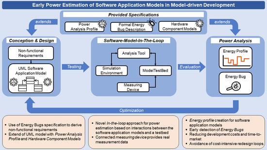
• A formal description and classification of energy-related bugs to specify energy-related NFRs. The concept of energy bugs is integrated into the automatic power analysis and evaluation of NFRs in early phases to optimize the software application model.
• A UML-based description of hardware components extended with a UML profile to model power-related aspects. The provided descriptions can be linked with the software application and provide interfaces for their utilization. Our approach can take the microcontroller unit (MCU) and connected peripheral devices into account, thus enabling a system-wide power estimation.
• Two methods for power estimation of software application models in MDD which are applied in different development stages. The indirect power analysis method provides a simulation-based rapid power analysis without needing an existing hardware platform. The direct power analysis method is based on a novel in-the-loop testing approach and uses a testbed for the estimation process. Additionally, the software application model can interact with the testbed, e.g., to obtain real measurement data from sensors during simulation.

To estimate the power-related impact of software application models, software-hardware interactions must be considered. The proposed approach offers concepts to model hardware components and integrates them into the software application model domain. The UML profile is based on MARTE and extends the concepts for a more detailed modeling of power-related aspects and the ability to consider dynamic changes. While initially presented in [15,16], the UML profile has been modified to integrate the concepts proposed in this article. Moreover, with the introduction of an analysis tool and defined protocols for message exchange, the presented approach is no longer limited to specific MDD tools for simulation and evaluation. The approach also enables the estimation and actual measurement of power consumption, which may be used along with the software model to derive an energy trace of the system as the key element for visualizing and detecting energy bugs in early development phases. We also provide an in-depth analysis of the efficiency of the direct estimation method for an IoT sensor node example and demonstrate how energy bugs can be defined and detected using the proposed concepts. To the best of our knowledge, this is the first approach to make the impact of non-functional aspects like power consumption of software application models in MDD visible. Software developers may utilize the provided energy model to estimate and improve the power-related behavior of software application models for embedded systems.

The remainder of this article is structured as follows: Section 2 discusses the background on power estimation, energy bugs, and in-the-loop testing. Section 3 summarizes the related work, while Section 4 introduces the IoT application example to which our concepts are applied. Section 5 presents an overview of the two analysis methods and the developer workflow. Section 6 introduces the concepts of hardware component models and the extended UML power analysis profile. Section 7 presents the exemplary implementation of our concepts and introduces software and hardware models for the IoT application. Section 8 provides an evaluation of the proposed concepts and energy bug detection. Section 9 discusses our approach, while Section 10 concludes this article.

2. Background

This section provides a formal definition of the power estimation process based on state machines as a key element of this article and a formal definition and classification of energy bugs. As another key element, this section briefly summarizes in-the-loop testing.

2.1. Energy Model of Hardware Components

In order to describe the underlying concepts of the proposed approach, this section aims to provide a brief definition to model the behavior of hardware components and theoretical background for calculating the power and energy needed to derive energy traces. The term embedded system S refers in this article to a hardware platform consisting of a finite set of n independent hardware components C, so that:

$$S=\{C_1,C_2,...,C_n\}$$

Each hardware component $C_i$ contains a finite state machine (FSM). For example, an embedded system may consist of a MCU, sensor, and radio module, as outlined in Section 4. The state of the embedded system S at a specific time is determined by the active state of each hardware component $C_i\in S$. The electric power $P_{C_i}$ and energy $E_{C_i}$ of a hardware component $C_i$ for a specific time point $t\in T$ can be expressed as:

$$\begin{array}{cc}\hfill P_{C_i}\left(t\right)& =V_{C_i}\left(t\right)·I_{C_i}\left(t\right)\hfill \end{array}$$

(1)

$$\begin{array}{cc}\hfill E_{C_i}\left(T\right)& ={\int }_{t=0}^T{P}_{C_i}\left(t\right)dt\hfill \end{array}$$

(2)

To calculate the electric power $P_{C_i}$ of a hardware component $C_i\in S$, the time-dependent supply voltage $V_{C_i}\left(t\right)$ and the time-dependent current consumption $I_{C_i}\left(t\right)$ are used and rely, for example, on the current state of the component. Similar to Equations (1) and (2), the electric power $P_{\mathit{S}}$ and energy $E_{\mathit{S}}$ of an embedded system S consisting of n hardware components $C\in S$ can be defined as:

$$\begin{array}{cc}\hfill P_{\mathit{S}}\left(t\right)& =\sum _{i=1}^n{P}_{C_i}\left(t\right)\hfill \end{array}$$

(3)

$$\begin{array}{cc}\hfill E_{\mathit{S}}\left(T\right)& ={\int }_{t=0}^T{P}_S\left(t\right)dt={\int }_{t=0}^T\left(\sum _{i=1}^n{P}_{C_i}\left(t\right)\right)\hfill \end{array}$$

(4)

Each state and transition defined in the FSM for a hardware component $C_i$ is annotated with power and timing aspects. These descriptions are used to calculate the actual power consumption based on Equations (1)–(4). To address RQ2, the presented definitions are part of the UML profile (cf. Section 6). The energy model abstractly describes the energy consumption of a hardware component and uses the physical relations in Equations (1)–(4). To describe the energy model, a UML profile as an extension for UML models (cf. Section 6) is developed in this article. The UML profile makes it possible to assign energy properties to state machines and class definitions. Furthermore, two methods (cf. Section 5.1) are presented to determine the energy consumption of an application on the system level. The result of these measurements is denoted as an energy trace. In order to distinguish between modeling (UML profile) and measurement, this article uses the term energy trace for measurement results which is synonymous with the term energy profile used in the literature.

2.2. Energy Bugs

The behavior of a system to consume more energy than required to fulfill the intended task is already known. The term energy bug to describe such behavior has gained more attention due to the increasing number of battery-powered embedded systems over the last few years. Researchers have published numerous works [17,18,19] to analyze energy consumption and to detect and describe energy bugs for smartphones and mobile applications [20,21,22]. Even if the basic findings and concepts are also valid for smaller embedded systems in the IoT domain, major differences exist. Due to this, the definition has to be revised. Unlike smartphones, embedded systems, especially in the IoT, have even more limited hardware resources like CPU power, memory, interfaces, and energy storage and operate on lower levels. These limitations can be more challenging for software developers. Additionally, while smartphones are more universal devices built on state-of-the-art components, embedded systems used in IoT are optimized for specific use cases. At the same time, software developers have to deal with less common and use case specific components, e.g., communication interfaces or sensors.

Common descriptions of energy bugs exist that mainly refer to the effects but do not provide a clear definition or specific sources of energy bugs [20,23]. For example, in [20], the categories of energy hotspots and energy bugs were presented. While an energy hotspot describes a high battery power consumption even if the utilization of hardware resources by an application is low, the definition of an energy bug only covers scenarios in which a malfunctioning application prevents the system (e.g., smartphone) from entering a lower power state (e.g., idle) after the execution is finished. However, the introduced descriptions are insufficient for software developers of embedded systems. First, software applications for embedded systems like IoT sensor nodes use special purpose and resource-efficient operating systems with less functionality. Second, a more precise control of individual sub-components of embedded systems is needed to address energy-related misbehavior that is not covered by the classification and examples mentioned in [20].

2.2.1. Definition

In this article, the term energy bug refers to an unintended behavior of an embedded system consisting of peripheral devices and a software application causing a higher power consumption, which is unnecessary to provide the current functionality. To address RQ1, we introduce a new definition that incorporates previous considerations and is more precise for embedded systems. To describe a non-conformant energy consumption of a system S, component $C_i$ or application, we introduce a tuple of two parameters $\langle E_{\mathit{qu}},I_{\mathit{dmax}}\rangle$. The energy quota $E_{\mathit{qu}}$ describes the energy available for a period T for the unit under consideration. The second parameter specifies the maximum demand current $I_{\mathit{dmax}}$. If a battery-powered system is considered, this corresponds to the maximum continuous discharge current. The behavior of a software application is generally dependent on the environment and context in which it is executed. This applies in particular to embedded systems such as IoT devices. As a result, the power demand and the power consumption are directly or indirectly influenced by the context. To address this behavior, we introduce the additional parameter $SC$ for a scenario and informally define $SC$ as a set of conditions and constraints that apply to a time period T under consideration. For example, the ambient temperature influences the energy quota since low temperatures increase the self-discharge of a connected lithium-ion battery. Poor network connectivity can result in multiple transmit or receive cycles increasing the power consumption of a wireless module.

Definition 1.

We define a system S (or a subset of components $C_i$) to beenergy bug-freeif the following two conditions (5) and (6) are satisfied for a given scenario $SC$:

$$\begin{array}{cc}\hfill E_S\left(T\right)& \le E_{\mathit{qu}}\hfill \end{array}$$

(5)

$$\begin{array}{cc}\hfill max\left(I_S\left(t\right)\right)& \le I_{\mathit{dmax}}\hfill \end{array}$$

(6)

Therefore, an energy bug infringes at least one of the two conditions and thus describes a deviation from a previously defined requirement. In addition to the faulty behavior, unused energy-saving opportunities must also be considered.

Definition 2.

We define a system S (or a subset of components $C_i$) to beenergy-awareorenergy-efficientif we apply a set of measures that minimizes $E_S\left(t\right)$ and/or $\mathit{max}\left(I_S\left(t\right)\right)$.

Such measures can be, for example, the application of a suitable design pattern, an optimizing compiler, or the replacement of an algorithm. It is important to note that these measures do not negatively impact the system’s functionality or other NFRs (e.g., safety, real-time behavior, response times). The approach presented in this article allows, on the one hand, to find and eliminate energy bugs and, on the other hand, to test and evaluate energy-efficient measures.

2.2.2. Classification

In general, energy bugs do not necessarily reveal themselves through the misbehavior of the software application itself. Thus, a functionally correct software application can still contain energy bugs resulting in increased power consumption and shorter battery life. Due to our research, energy bugs can arise from different sources, which can be classified into broad categories:

• Type A: An incorrect hardware design or faulty hardware component leads to increased power consumption during runtime. The cause of such an error can be, for example, in the layout and become visible due to changed environmental conditions.
• Type B: Unknown or unconsidered consumers, which can be hardware or software components, lead to an increased power demand. For example, additional LEDs in the layout indicating a correct operation increase the power requirement.
• Type C: Energy bugs in this category are mainly caused by the software application itself. Flaws in the software design, incorrect utilization, or inappropriate design patterns [14] may lead to higher power consumption. Hardware components may also have a fixed energy offset described as ramp and tail energies [20,24] before and after the execution of tasks. The offset substantially affects the overall consumption if these operations are executed at a high frequency. Examples of avoidable additional power consumption are unnecessarily high sampling rates of sensors.
• Type D: Components such as MCUs and peripheral devices realize a sleep mode that is activated when the component is not accessed. Unintentional accesses can thus prevent these components from switching to a sleep mode (no-sleep bug [25]). Peripheral devices can also be bound too early or too long in specific parts of the software workflow. As a result, they may persist in a high-power state longer than necessary.

The causes of bugs in categories A and B are mainly located in the hardware layer of the system. In many cases, troubleshooting cannot be done by software, and, in the worst case, the hardware must be replaced, or the layout reworked. Type C and D energy bugs are mainly related to the software of the embedded system. However, Type D errors can be considered as a special case of Type C errors. Due to the frequent occurrence of Type D errors, they are assigned to a separate category. With the energy quota $E_{\mathit{qu}}$ and the maximum demand current $I_{\mathit{dmax}}$, indicators and threshold of energy bugs can be quantified. Considering Definitions 1 and 2, Equation (5) may be used to specify an indicator for all types of energy bugs, while Equation (6) may be used to define thresholds for Types A–C.

2.3. X-in-the-Loop Testing

If software applications are developed using model-based methods, in-the-loop tests may be performed as a consistent testing process from the initial (partial) model to the finished system [26,27]. For early steps in the development process, model-in-the-loop (MIL) tests may be applied where only the system under test (SUT) and an environment simulation are required. MIL can be executed without an existing hardware platform (e.g., IoT node) and relies only on model representations. Due to this, MIL tests are used in early development phases where the model itself or independent parts of the model may be evaluated. In hardware-in-the-loop (HIL) tests, the software application model is executed on the hardware platform (e.g., the prototype of an IoT node). Such tests are typically performed in later development phases and used as integration and system tests to identify software and hardware platform-related problems. Other approaches like software-in-the-loop or processor-in-the-loop are not discussed in detail because the verification of the generated platform-specific source code of the software application model and its execution on the target hardware are not related to the concepts presented in this article.

The aforementioned approaches mainly evaluate the software application model for intended behavior. The software application model can be fully operational and functionally correct while power-related NFRs (e.g., maximum peak power or battery lifetime) may not be met. Without adjusted test setups, such requirements can only be evaluated during the end of the development phase, resulting in increased rework phases and higher costs. The presented concept of this article utilizes the concepts of MIL and HIL in an adapted manner to obtain energy traces as the energy footprint of a software application model when interacting with a testbed. To summarize the concepts for the following sections, this article introduces the term software-model-in-the-loop as an in-the-loop approach for a software application model with an integrated energy model.

3. Related Work

Many research efforts use various techniques to address power consumption estimation for embedded systems on different abstraction levels. Low-level approaches at transistor level, gate level, and register transfer level (RTL) [28,29,30] offer highly accurate simulations but require a deep understanding of the internal structure of the hardware component to be modeled. Due to the complexity, these techniques are often used to simulate single components or intellectual properties (IP) of a component. Because of the hardware-specific modeling and extensive simulation times, they do not become relevant for software developers who want to optimize the software application.

Instruction-level power analysis (ILPA ) and functional-level power analysis (FLPA) may be used on higher levels. ILPA estimates the power consumption based on instruction and instruction pairs [31,32,33]. Software applications in high-level languages must be translated into assembly language, while instruction set simulators may be used for evaluation and analysis [34]. The energy cost for each instruction has to be measured in detail using experimental environments of the CPU, which can quickly become unmanageable for complex architectures with large instruction sets. FLPA decreases the time needed to build energy models. As function-level power estimation first mentioned in [35], built-in library functions as a sequence of instructions and user-defined functions as a combination of both are used to estimate the power consumption. FLPA, however, is focused on the functional level of the CPU itself. For this, the CPU is modeled as a block [36] or divided into multiple functional blocks [37,38]. The consumption then depends on algorithmic and configuration parameters. Both ILPA and FLPA perform power estimation at the assembly level. FLPA has also been extended for the C programming language [36]. Again, they are focused on estimating the power consumption for single components, primarily the CPU, and are not intended to be used for a system-wide analysis of software applications interacting with other devices. In general, low-level methods based on assembly or specific programming languages are not relevant for software developers in MDD because the generation of platform-specific source code is ideally performed at later stages of the development process automatically. Other approaches like [39] may be used in later stages to optimize generated source code on the task level considering MCU-specific properties.

Besides theoretical models [40,41] to address power estimation on higher abstraction levels, other work [42,43] has been published focusing on the system level, where multiple components are modeled as functional blocks and state machine representations. Additionally, the combination of power states from different components is used to specify workflows representing the power-related behavior of the system [44]. However, they do not consider the integration into a model-driven concept.

In [45], a model-driven hybrid power estimation approach for embedded systems based on cycle- and bit-accurate simulations in SystemC [46] is proposed. The approach focuses on the CPU, cache and shared memory, and communication buses as part of a system on a chip (SoC), while the consumption models for the aforementioned components are designed as black-box and white-box models. A white-box model is integrated into the SystemC source code of a component and counts the occurrences of each state, while black-box models are additional modules connected between components to determine the current state of a component based on exchanged signals. Both models can be used concurrently in the simulation, resulting in the hybrid concept. However, the approach presented in [45] is not intended to consider a complete embedded system. Additionally, if the system consists of multiple complex components, e.g., dedicated sensors or wireless modules, an in-depth analysis of each component must be done to derive the behavior of internal memory and communication buses. This is especially true if components are black boxes and vendors do not provide detailed information. While our approach focuses on the software application level and software-hardware interaction for the estimation process, their work is more concerned with the design space exploration of SoCs. Furthermore, our approach considers black-box and white-box modeling but only defines a single state machine for each hardware component, reducing the time-related overhead during simulation.

A framework for a model-driven architecture to estimate the power consumption of near field communication (NFC) devices is presented in [47]. The proposed modes are based on SystemC, where each module (e.g., hardware component or peripheral device) is extended with a power state machine. Furthermore, use cases defined as sequence diagrams represent the software application. Although the basic idea to integrate physical hardware into the simulation process is similar to ours, the power estimation of the presented approach is limited to use cases for the communication between the NFC-Reader and NFC-Bridge, supplied by the NFC-Reader during communication. Our approach instead is designed to consider the complete system. A more fundamental difference compared to [47] is that our approach aims to evaluate software application models that will later be executed on the system connected to the simulation instead of additional components (e.g., NFC-Readers) connected to an existing system.

Another approach for a system-level power and energy estimation based on the architecture analysis & design language (AADL) is presented in [48,49]. The authors focus on power estimation of real-time operating systems, field-programmable gate arrays (FPGAs), and data transfers for the Ethernet communication of client-server architectures, as presented in [50]. In AADL, software components consist of data, threads, and process components and are bound to hardware platform components (e.g., CPU, buses, and memories). On the other hand, our approach is based on class and state machine definitions and uses the same concepts to model software and hardware components. Instead of using the property extension language of AADL, our approach focuses on software application models based on UML as the most used modeling language in the embedded software industry [12]. Our approach considers embedded systems typically used in IoT and IIoT consisting of an MCU, sensors, and actuators, rather than focusing on FPGAs. Additionally, our power analysis profile is based on MARTE, which is compatible with AADL component models [13,51]. As part of the estimation process, software and hardware platform components are extended with PowerBudget, EnergyBudget, and PowerCapacity properties, which are calculated in a two-step process. The basic power model for each hardware component is defined as a set of consumption laws for different parameter combinations. However, the consumption laws specified as linear equations are not integrated into AADL models. In contrast, our approach provides model annotations for all power and time-related properties as well as methods to define the dynamic behavior of hardware component models enabling a model-to-model transformation without loss of information.

An approach for power estimation and optimization of CPUs using UML profiles is proposed in [52]. The application is modeled at the task level, while the CPU model consists of a state machine with associated operations modes, defined as a tuple of voltage and frequency values and thresholds for over- and underutilization. For each additional operation mode mapped to a logical state of the CPU (e.g., execution, sleep, and idle in [52]), an additional state has to be defined, which makes the approach prone to the state explosion problem [53]. State transitions are executed at the start or end of a task based on the current utilization of the CPU. While our approach focuses on the application level and interactions between software and hardware components, their work is concerned with finding the best CPU utilization while not taking any other components of the system into account. Moreover, the approach does not consider the dynamics originating from the application. For example, it is not possible to adjust the frequency within a task, e.g., based on external events. Additionally, no measurements were performed to validate the results.

There are also approaches in MDD to model software applications and hardware aspects of embedded systems for a power consumption estimation based on UML and MARTE. In [54] and follow-up work [55], an approach for energy-aware scheduling and timing analysis of software applications is presented. The concept is similar for both approaches and is based on a timing-energy analysis model obtained by reverse engineering processes of existing source code resulting in UML class representations. However, the timing-energy analysis model does not include any implementation details. As a result, the evaluation is based on task level and predefined execution times. While our work is able to take dynamic behavior and multiple hardware components into account, their work focuses on analyzing the power consumption of the MCU.

Another profile based on UML and MARTE for power consumption and real-time analysis of embedded systems is proposed in [56]. Stereotypes of the profile provide tagged values for properties such as the switching capacitance, energy consumption per clock cycle, and voltage-frequency pairs as working modes of CPUs. While batteries are extended with voltage and capacity descriptions, other components like displays are limited to their static power consumption. To consider the software application, tasks without implementation details are defined and annotated with their execution interval and worst-case execution time and cycles instead. The simulation calculates the most power-efficient task-by-task working mode for a CPU while respecting real-time requirements of every task and task chains. However, the proposed approach focuses on executing inalterable tasks on CPUs, while our approach is designed to integrate the software application into the estimation process. By providing stereotypes for class and state machine diagrams, both static and dynamic aspects of hardware components can be considered.

As an extension of MARTE, the authors in [57,58] introduce a profile to address system-wide dynamic power management (DPM) aspects of embedded systems. The system-level view is achieved by defining power configurations. A power configuration specifies the state of each hardware component while the current configuration is active. The behavior of a hardware component is modeled with state chart diagrams. The DPM profile provides stereotypes to add power-related meta descriptions to states and transitions, e.g., frequencies, static and total power. The concept introduced in [58] provides two different approaches for the DPM profile. The first approach defines a power state machine of a many-core CPU, including states for each core configuration with associated power configuration. Based on over- and underutilization measurements, the number of active cores can be adjusted during simulation. In the second approach, the software application is modeled as use cases, e.g., boot, idle, and associated with a specific power configuration. The concept of dynamics is limited to the idea that hardware components may have different states depending on the active use case. However, configuration details of hardware components are considered only slightly. Due to the lack of integration of software application models, the presented approach offers no support for software developers for optimizations based on quantifiable values resulting from the simulation and evaluation. This also includes the detection of energy bugs located at the application level. However, while our approach introduces two analysis methods, which may be applied in different development phases, their work is defined at the conceptual level, with no evaluations performed using simulations, physical hardware components, or measurements.

Finally, to the best of our knowledge, with the presented concepts in this section, software developers cannot predict the impact on the power consumption of software application models for embedded systems. Furthermore, misbehavior of software applications such as energy bugs is not addressed. In contrast, this article presents a novel approach that enables a power consumption estimation of software application models in early development phases. We provide a formal definition of energy bugs and present an analysis tool to derive energy traces of software application models using simulation data or our novel in-the-loop approach. For this purpose, the analysis tool is able to control measuring devices and interact with testbeds as an executing entity. The resulting energy trace may be used to evaluate power-related NFRs and to detect energy bugs. Our approach may be integrated into the development workflow to achieve a concurrent and continuous evaluation of power-related aspects. Moreover, we extensively evaluate our concept using an IoT application example with a fully functional software application model evaluated in a simulation and model-in-the-loop environment.

4. IoT Application Example

This section describes a beehive microclimate sensor node to monitor western honeybee (apis mellifera) colonies shown in Figure 1 as an IoT application to demonstrate the process of hardware component modeling and annotation (cf. Section 7.3) and to evaluate the overall performance of the presented approach (cf. Section 8.2).

In general, beekeeping in magazines made of wood or polystyrene can negatively affect bees since the magazines do not correspond to natural housing. Bees can actively influence the humidity of a magazine to ensure optimal environmental conditions for larvae and the colony [59]. The sensor node monitors the actual condition in the magazine and propagates the environmental data over a wireless communication interface. A block diagram of the sensor node is shown in Figure 2 and consists of an Espressif ESP32 MCU [60] and a Bosch BME280 environmental sensor [61] connected via the inter-integrated circuit (I²C) which is placed inside the beehive magazine measuring temperature, humidity, and air pressure.

For energy-efficient and long-range wireless communication, a long-range wide area network (LoRaWAN) [62] is used to transmit sensor data obtained by the BME280 to an open IoT infrastructure with a cloud service such as The Things Network (TTN) [63]. To extend the sensor node with LoRaWAN capabilities, a RAK Wireless RAK811 WisDuo LoRa module [64] based on the Semtech SX1276 LoRa transceiver [65] is connected via the serial communication interface universal asynchronous receiver-transmitter (UART). The sensor node is configured as LoRaWAN class A device [66], which represents the most energy-efficient type of end device defined in the LoRaWAN specification [62]. As the main characteristic of class A devices, the communication can only be initiated by the end device with an uplink message resulting in a transmit (TX) window. After transmitting data, a first receive (RX) window is opened, followed by a second RX window if no downlink message has been received during the first RX window. While using the prototype of the IoT sensor node, as shown in Figure 1, an unexpected behavior was observed, resulting in a depleted battery within a few days. The concepts presented in this article are intended to demonstrate how such misbehavior can be addressed in the early development phases of the software application.

5. The Proposed Power Analysis Concepts and Developer Workflow

This section describes the overall concept of the power analysis process and presents a developer workflow, which describes the individual steps if the power analysis process is integrated into the software development workflow.

5.1. Power Analysis Concepts

The framework offers two main estimation concepts to derive energy traces, which can be used in different phases of the development process in MDD. The first estimation concept presented in this article and shown in Figure 3 is described as indirect power analyses (IPA) and can be applied to very early development phases where the hardware platform may not be available or defined yet. It relies on energy models for each hardware component and is based on estimated current consumption values of individual hardware components.

The main concept was introduced in [15] but has been redesigned and extended due to recent research findings. The MDD tool in Figure 3 is used to design the software application model and hardware component models. Additionally, the MDD tool may offer a simulation environment where the software application model can be executed. Compared to the previous approach, a central tool for the simulation and analysis has been defined. The analysis tool directly interacts with the simulation environment provided by the MDD tool to trace all hardware accesses of the simulated software application, which can lead to changes in the energy-related behavior of one or more hardware components. Additionally, data values for hardware components (e.g., measurements) can be predefined and passed to the simulation if, e.g., a sensor is activated to collect data. By this, scenarios (cf. Section 2.2) as an environment definition for simulating software application models can be realized. The second concept, shown in Figure 4, is called direct power analysis (DPA) and implements the software-model-in-the loop approach. It introduces a procedure in which software-hardware interactions are generated in the simulation, forwarded to a hardware platform (ModelTestBed), and reproduced by a message interpreter instance. Since our approach focuses on deriving energy traces to evaluate NFRs, only software-hardware interactions instead of the complete software model have to be replicated on the ModelTestBed. Each instance of a hardware model in the simulation of the MDD tool is linked to s specific peripheral device on the hardware platform, which addresses RQ3. This article focuses on concepts provided by DPA for the implementation of the power analysis process (cf. Section 7) and the evaluation (cf. Section 8) since all concepts of IPA are also used in the DPA approach.

For IPA and DPA, we developed the unit for central control and estimation (UC²E) tool (cf. Section 7.1) as a central component to provide analysis and control functionalities. A measuring device is connected to the ModelTestBed for continuous voltage and current measurements. The measured values are accumulated and evaluated by the UC²E tool. Since the UC²E tool is aware of the internal state of each hardware component based on trace data sent by the simulation, state and state transitions of each hardware component model can be mapped to a specific time or time frame of the measurement. Due to this, an extensive power analysis can be achieved, which leads to more detailed energy traces. The proposed approach has been designed as a modular architecture, enabling the rapid development of new setups for specific test cases. The communication interface between the simulation and the UC²E tool is independent of a specific MDD tool, enabling the usage of different MDD tools such as MathWorks MATLAB or IBM Engineering Systems Design Rhapsody–Developer [67,68], abbreviated as IBM Rhapsody in the subsequent sections. With ModelRPC (cf. Section 7.2) for the communication between the UC²E tool and the ModelTestBed, we defined a novel communication protocol to provide universal control and management of hardware resources. Hence, the ModelTestBed is not limited to specific controller platforms and allows the integration of peripheral devices dynamically to evaluate power consumption. Additionally, the ModelTestBed may be used to provide actual data (e.g., sensor measurements) for the simulation of the software application model. This approach also supports different types of measuring devices due to the integration of universal communication protocols like the standard commands for programmable instruments [69] and the virtual instrument software architecture standard [70,71].

5.2. Developer Workflow

In addition to the introduced power analysis concepts, this section illustrates the developer workflow. The UML activity diagram in Figure 5 describes the different steps and resulting artifacts starting with the development towards the evaluation and analysis of the software application model. The first actions 1(a) and 1(b) in Figure 5 describe the definition of functional and non-functional requirements and the creation of a suitable hardware component list, resulting in artifacts A1 and A2. The artifact A1 also includes defined scenarios $SC$, energy quotas $E_{\mathit{qu}}$, and maximum demand currents $I_{\mathit{dmax}}$ (cf. Section 2.2), which are used in later steps to detect energy bugs. Based on the specifications (A1), a functional UML model of the software application (A3) is created in step 2. In parallel, hardware component models are created in steps 3–4. It is possible to import hardware component models into an existing project using a model repository or to create new models and use the power analysis profile (PAP) to apply a set of power-related stereotypes. The energy model for a hardware component is defined by using PAP to describe power and time-related aspects. The results are multiple objects (artifact A4) representing abstractions of hardware components that can interact with the software application model. Step 5 integrates the software application model (A3) with hardware component models (A4), resulting in a system model (A5). The last step 6 of the development process includes a model-to-text transformation of the hardware component models using the JSON-based interchange format presented in [15]. Step 7 describes the import of the hardware component model descriptions into the analysis tool as the first step of the evaluation process. Based on the information provided by PAP, an energy model of each hardware component for the analysis during simulation can be derived. In step 8, the test environment is configured before the software application model is simulated in step 9. As a result of the simulation, the energy trace (A6) is obtained, analyzed in step 10, and compared to the specified requirements (A1). If power-related requirements are not met, or energy bugs are not detected, the software application model is optimized by fixing detected energy bugs in step 11. Afterward, the analysis process is repeated, starting with step 9. Note that steps 4–6, shown in Figure 5, can be executed automatically, e.g., due to extensions implemented for the MDD tool.

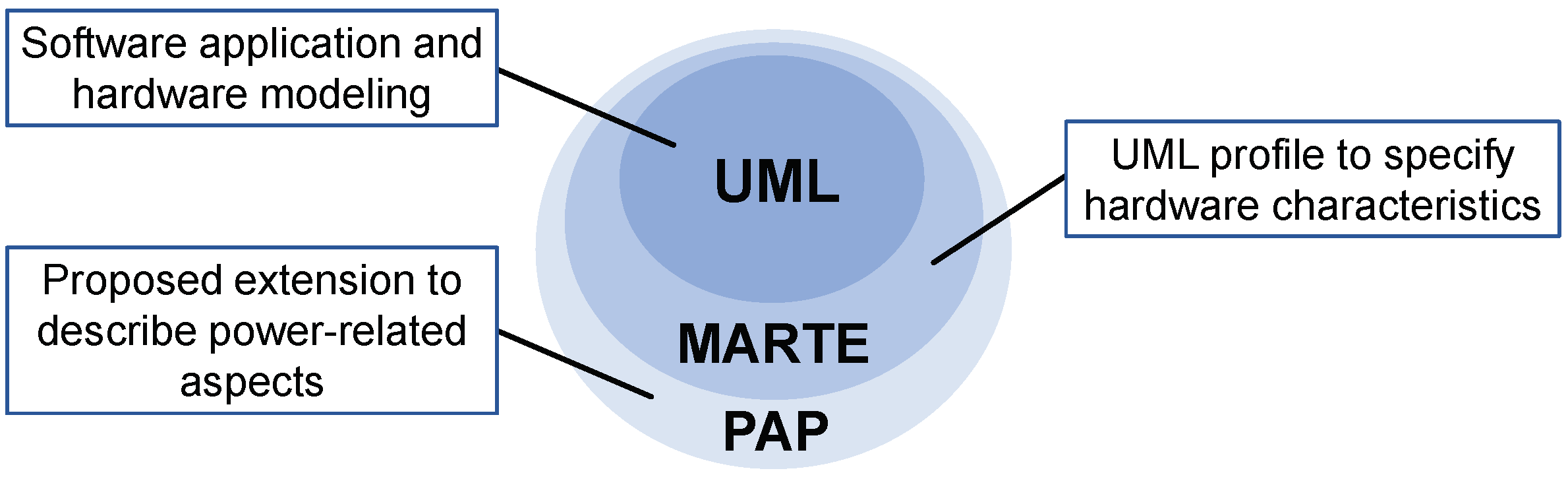
6. The Proposed Hardware Component Model and Power Analysis Profile Specification

This section describes the specification of hardware component models based on concepts provided by UML and PAP as the key approach to model non-functional aspects. Figure 6 shows the relation between UML used to define hardware component models, MARTE as an extension of UML, and the PAP to model power- and timing-related aspects based on MARTE. The presented concepts in this section address RQ1–2 and are conceptually located in part 4 of the developer workflow shown in Figure 5. Furthermore, a dimmable LED as an exemplary hardware component model is presented across Section 6.2 and Section 6.3.

6.1. Hardware Component Model Specification

To enhance the understanding of the overall approach, this section summarizes the main components of a UML-based modeling hardware component model as a basis for the PAP. The general structure of hardware component models follows the hardware proxy pattern [72] and also offers the possibility of considering non-functional aspects. When modeled with UML, hardware component models are represented as UML classes (referred to as proxy class in [72]) extended with behavioral state machines applied as classifier behavior [10]. States of the behavioral state machine represent operational states of the physical hardware component while transitions lead to state changes initiated, for example, if operations of the proxy class are called within the software application model. To enable a communication for the IPA and DPA concepts (cf. Section 5.1), a policy-based device pattern as a hardware abstraction layer (HAL) introduced in [16] is used. Furthermore, elements of the UML class and state machine definitions can be annotated with the PAP (cf. Section 6) to model non-functional aspects. State machines used in the context of hardware component models are also referred to as power state machines [73].

6.2. Overview: Power Analysis UML Profile

The basic idea of the UML-based PAP shown in Figure 7 is to use stereotypes to annotate different types of UML elements with power-related meta information. The profile is based on MARTE [13] and designed to be applied on hardware component models, e.g., as described in Section 5.2 during the development process, located in step 4(b) of the developer workflow shown in Figure 5.

The basic definition of the PAP was first published in [15] but has been modified and expanded based on the novel concepts presented in this article. PAP is designed to annotate UML-based models and provides a set of stereotypes that can be applied to different UML elements to extend the semantic description. All defined stereotypes are assigned to one of the two sub-profile packages based on their particular purpose shown in Figure 7 and may be used to specify power-related aspects of UML-based hardware component models. Stereotypes for class definitions of hardware component models are described in Section 6.2.1, while Section 6.2.2 introduces stereotypes for behavioral state machines. Section 6.3 covers the concept of mapping dynamic energy-related behavior via stereotypes.

6.2.1. Hardware Abstraction Model with Energy-related Elements

Stereotypes of the HardwareAbstraction sub-profile package are designed to provide additional information for UML class elements, e.g., operations and attributes, of a hardware component model. Figure 8 gives an overview of the stereotypes provided by this package.

The stereotype HWDeviceAbstraction specifies hardware component models in the model application and provides tagged values for basic properties, e.g., the supply voltage and supported frequencies. Since the data types provided by MARTE are not sufficient for this approach, an additional data type with the name NFP_Voltage is defined in PAP to specify the electrical voltage of a hardware device and to provide rules for conversion between units. If attributes of the UML class affect the execution time or the current consumption of a hardware component model, they can be annotated with the HWPowerAttribute or HWTimingAttribute stereotype, respectively. With the provided tagged values, developers can configure a unique id of the attribute to implement dynamic power-related behavior as described in Section 6.3. The remaining tagged values direction and type describe further properties of attributes, which can be included in model-to-model or model-to-text transformations. The stereotype HWBehavioralImpact is used to annotate all functions, which can affect the power-related behavior of a hardware component model or manipulate values of attributes annotated with the stereotypes HWPowerAttribute or HWTimingAttribute. Note that stereotypes for operations are mainly used as an identifier for later model transformation processes. For example, if such operations affect power- or time-related attributes, additional automatic source code generation steps [74] may be performed prior to the simulation to extend the opaque behavior with additional trace commands, including affected attributes and their new values.

To illustrate the usage of stereotypes provided by the HardwareAbstraction package, the class definition shown in Figure 9 describes the structure of the hardware component model for the dimmable LED. The class DimmableLED inherits from PeripheralDevice as one of two base classes specified in [15] to provide a set of predefined operations for the interaction with the software application, e.g., to turn the device on or off. The DimmableLED class provides an attribute brightnessLevel to represent the current brightness of the LED, which can be changed by the software application using the setBrightness method. The attribute is annotated with the HWPowerAttribute stereotype to specify an id for later usage in expressions. The PercentageInteger data type of the attribute may be used to derive test data in later steps. The definition shown in Figure 10 follows MARTE [13] concepts and includes boundary definitions. Note that the generation of test cases is outside the scope of this article. However, PAP has been designed to be compatible and used along with MARTE.

6.2.2. Hardware Behavior Model with Energy-related Elements

The HardwareBehavior sub-profile package provides stereotypes to apply the concept of power state machines [73] to UML behavioral state machines [10]. Figure 11 shows the stereotypes provided by the HardwareBehavior package and the corresponding UML elements to which the stereotypes can be applied. A power state machine does not need to cover and describe all logical operation modes. For example, two operation modes can be aggregated if they cannot be observed or distinguished externally (black box behavior) or if they do not have different current consumption values and thus have the same impact on the overall power consumption. On the other hand, an operation mode of a hardware component can be separated into different power modes if the operation mode has a varying consumption characteristic for different phases, e.g., if a measurement state of a sensor consists of a pre-head and a data collection phase.

A state machine may be extended with the stereotype HWDeviceBehavior if it represents a power state machine. The stereotypes HWDeviceBehavioralState and HWDevice-BehavioralTransition are applied on UML states and transitions to provide the following set of tagged values, namely:

• hasDynamicConsumption: Defines if the consumption of the state or transition is variable or static.
• hasDynamicExecutionTime: Defines if the execution time of the state or transition is variable or static.
• current: Contains the electric current consumption of a state or transition.
• executionTime: Contains the execution time of the state or transition.

An additional non-functional property (NFP) data type NFP_Current has been defined in PAP and applied on the tagged value current to represent electric current with the base unit ampere. For states, the tagged value executionTime can be left empty if the current state is maintained until an external source initiates a state transition, e.g., turning a hardware component on and off. The two stereotypes hasDynamicConsumption and hasDynamicExecutionTime define whether a state or transition has a static or dynamic current consumption or execution time. All stereotypes of this package inherit from the ResourceUsage stereotype of the MARTE profile [13]. Due to the inheritance, additional tagged values such as msgSize or allocatedMemory are available and may be used to provide further domain-specific descriptions. To aid in readability, only stereotypes introduced by PAP are shown in Figure 11. States and transitions may also contain simulation-dependent source code to realize behavioral characteristics and calculate delays.

The state machine shown in Figure 12 defines the behavior of the dimmable LED and consists of the two states On and Off. Instructions defined in class operations, e.g., powerOn() and powerOff(), generate events to initiate state transitions. Both states are annotated with the proper stereotype of the PAP. For state Off, the consumption is set to 0 mA while the state On has a dynamic consumption indicated by the tagged value hasDynamicConsumption. Assuming that each state change is instantaneous, the tagged values current and executionTime for transitions between the two states On and Off are set to 0 mA and 0 ms, respectively.

6.3. Managing Dynamic Power-Related Behavior

For an energy model, it is necessary to define the current consumption and the execution time for each hardware component state. The current consumption and execution time can be specified as a fixed numeric value if they are static and do not change during execution, as described by the related approaches in Section 3. However, both values may become time-dependent when affected by the software application resulting in varying values during runtime. This section presents a concept to consider the power-related behavior for the analysis process. Note that even if only states are annotated in the example of the dimmable LED, the same concept can also be applied to transitions.

The tuple notation (value, expr, unit, statQ, dir, source, precision) of NFP types specified by MARTE [13] structures the content of tagged values (e.g., current and execTime) provided by stereotypes of the PAP. In this approach, only the elements value, expr, and unit are used to describe tagged values, e.g., (20, mA) or (5·20, ms). While the unit element is mandatory, either the value or the expr element has to be defined depending on the use of static values like fixed numbers or dynamic values defined as expressions. Optionally, the element source may be used the specify if the value, e.g., current consumption, has been derived from the datasheet as an estimation (source = est), obtained by an actual measurement (source = meas), or calculated (source = calc). Note that the use of the source element has only an informal character with no effect on the processing of NFP types. As introduced in Section 6.2.1, attributes of a class can affect the power consumption of a hardware component model. For such conditions, expressions described with the value specification language (VSL) [13,75] are applied. Our approach requires cross-references between tagged values of different UML elements to reflect dynamic behavior in the model definition. The declaration and usage of variables defined in the VSL::Expressions package of the MARTE specification have been slightly enhanced. Changes are described in Listing 1 using the extended Backus–Naur form (EBNF).

Listing 1. Selected parts of the value specification language specification for variables described in extended Backus–Naur form. A definition of the nonterminal symbol 〈init-expression〉 can be found in [13]. Adaptations are highlighted in bold.
〈variable-call-expr〉	⊨	〈variable-name〉
〈variable-declaration〉	⊨	[〈variable-direction〉] ‘$’ 〈variable-name〉
		[‘:’ 〈typename〉] [‘=’ 〈init-expression〉]
〈variable-direction〉	⊨	‘in’ | ‘out’ ‘ | inout’
〈variable-name〉	⊨	[〈namespace〉 ‘.’] | 〈body-text〉
〈namespace〉	⊨	〈pap-prefix〉 [ ‘.’ 〈pap-postfix〉 ] 〈body-text〉
〈pap-prefix〉	⊨	‘PAP’
〈pap-postfix〉	⊨	‘SM’ | ‘ATTR’
〈body-text〉	⊨	terminal symbol consisting of string of characters

By defining a dedicated namespace as a separation between the basic concepts of MARTE and the extension provided by PAP, the compatibility between MARTE and PAP is maintained. The main reason for the extension shown in Listing 1 is to define object-level cross-references and references between objects and their structure and behavior. This results in the following set of rules if an MDD project makes use of PAP:

• If a variable for PAP is defined, the namespace has to start with a specific prefix, while the use of the postfix is optional and depends on the type of reference.
• For the prefix, the term PAP has to be used.
• The postfix can be one of the two terms SM or ATTR.

To access the bounds attribute of the IntegerInterval type (cf. Figure 10) for the dimmable LED defined in package Pkg, the namespace Pkg.DimmableLED.brighnessLevel. bounds has to be used. However, while properties of a data type for a specific class attribute are constant, values of attributes become instance-related and differ for each class instance. Two instances of a sensor class, for example, can be configured differently and therefore have various current consumption values when performing a measurement. These instance-related values are necessary for an analysis of power consumption. To include the value of the brighnessLevel in equations of tagged values provided by PAP, the reference PAP.ATTR.brightness may be used where PAP indicates the usage in the context of the profile, ATTR refers to an attribute of the class annotated with the aforementioned stereotypes, and brightness refers to the tagged value id. However, this concept is not limited to attributes and can also be applied to cross-reference tagged values for state machine elements. For example, PAP.SM.NameOfState.NameOfTag references a tagged value of another state. To refer to a tagged value in the scope of the current UML element, e.g., state or transition, the definition PAP.NameOfTag may be used. However, the interpretation of namespaces is not defined in the MARTE specification and has to be implemented by the analysis tool. During a model transformation, the stereotypes HWPowerAttribute and HWTimingAttribute may be used to extract the <variable-direction>, <variable-name>, and <typename> described in Listing 1 by using the tagged values direction, id, and type, respectively.

To conclude the example of the dimmable LED, the dynamic behavior is modeled with the concepts introduced in this section. The current consumption for the On state, as shown in Figure 12, can vary between 0.05 mA and 5 mA due to the definition of the interval $[1,100]$ for the type of the attribute brightnessLevel (cf. Figure 10). Instead of defining multiple states to cover each possible current consumption, our profile prevents state explosion [76] and addresses such dynamic behavior. The expression used to calculate the current consumption includes the previously defined reference PAP.ATTR.brightness, as shown in Figure 12. A software application model can modify this attribute during simulation, resulting in a reevaluation of all expressions that include the tagged value. While this type of dynamic behavior introduced by PAP is not specified in MARTE, analysis tools (cf. Section 7) have to keep track of changes for all variables annotated with the HWPowerAttribute stereotype during execution to make an evaluation possible.

7. Implementation of the Power Analysis Process and IoT Application

This section describes the implementation of the power analysis process based on the concepts introduced in Section 5 and Section 6 and gives a brief overview of the technologies used.

Additionally, this section covers the implementation of the beehive microclimate sensor node as the IoT application example introduced in Section 4. Figure 13 shows a concrete implementation of the DPA concept previously introduced in Section 5.1. In the following subsections, the specific parts of the concept are described in more detail. An overview of the UC²E tool, marked as (A1), and the communication protocol between the UC²E tool and the simulation (A2) are given in Section 7.1. Additional extensions for a model transformation of the hardware component models have been developed to export energy-related information from IBM Rhapsody (dashed line in Figure 13), used for the analysis process in the UC²E tool. A description of the JSON-based representation format used for the model transformation can be found in [15]. The architecture and functionalities of the ModelTestBed (B1) are introduced in Section 7.2. In addition, ModelRPC (B2) as a communication protocol between the UC²E tool and the ModelTestBed is also part of Section 7.2. Section 7.3 covers the implementation of the UML model for the beehive microclimate sensor node representing (C) in Figure 13. As a UML modeling tool and simulation environment for UML-based models, IBM Rhapsody in Version 9.0 [68] is used while measurements (D) are performed with a Qoitech Otii Arc [77].

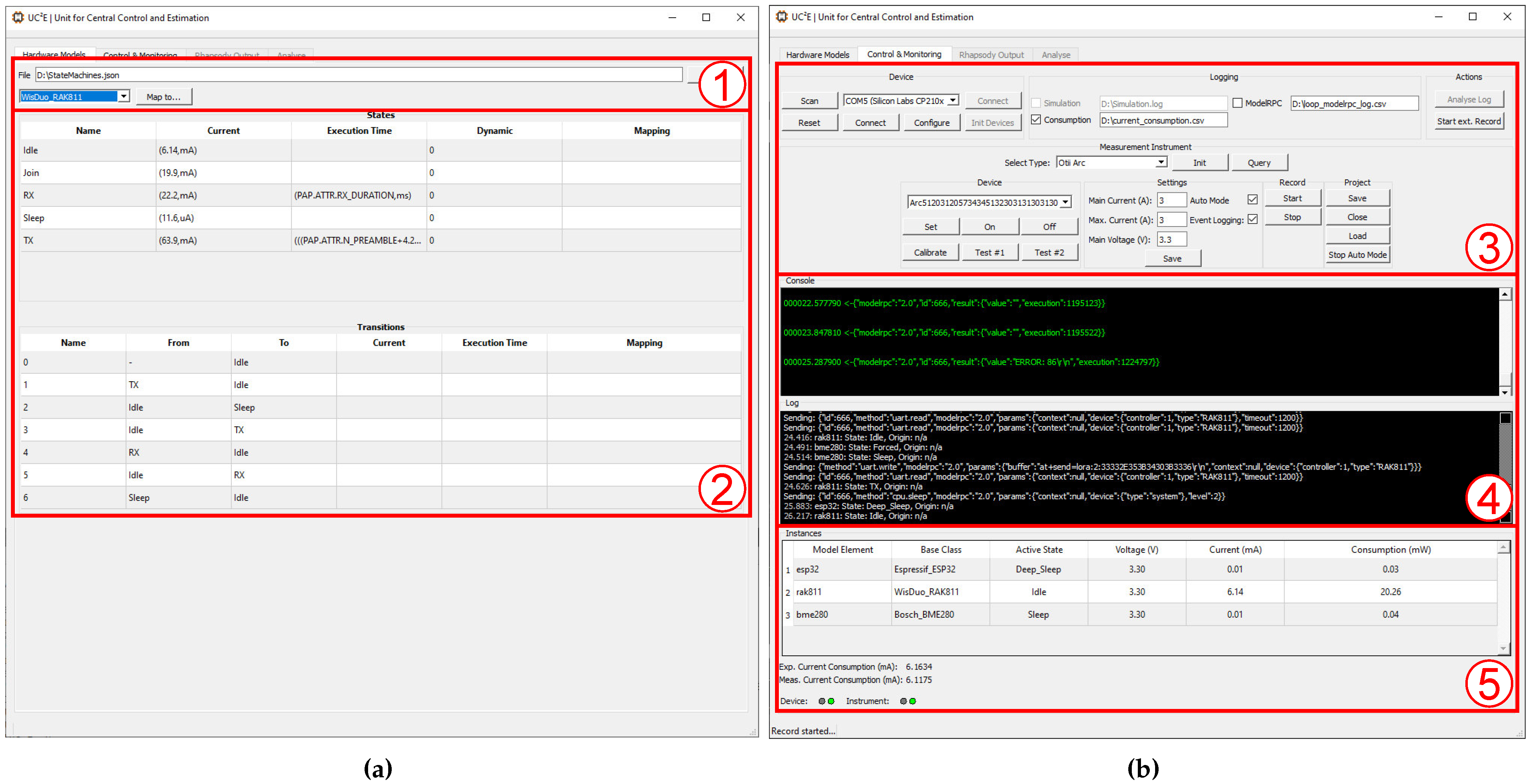
7.1. Unit for Central Control and Estimation

We developed the UC²E tool that enables developers to estimate the power consumption of software application models in MDD. It can perform a power estimation and energy bug detection based on the two concepts presented in Section 5.1. As the central element of the presented approach, it defines the test and runtime analysis environment for software models by providing interfaces to connect measurement devices and executable environments. Figure 14 shows two views of the developed prototype.

With the first view shown in Figure 14a, developers may import (1) state machines of hardware component models described in the JSON-based interchange format previously presented in [15] to configure the UC²E tool. Furthermore, the extracted energy model for each hardware component is displayed, highlighted as (2) in Figure 14a. The developer can adjust the tagged values of states and transitions provided by PAP if necessary. Figure 14b shows the Control & Monitoring view, in which the developer can establish the connection to the ModelTestBed, configure and control the measuring unit, and initiate a diagram generation (3). The middle part shows the live analysis features with two output windows for the ModelTestBed communication and the interaction with the simulation environment, including request and response simulation messages (4). The lower part of Figure 14b contains a table with instances of hardware component models (5) used in the current simulation and their active states and expected current consumption. Additionally, the estimated and measured current consumption is displayed in this view.

In order to provide a bidirectional communication protocol between the simulation environment and the external UC²E tool (cf. Figure 3), a message exchange format has been specified containing the message types register, behavior, and action. These message types enable a well-defined exchange of trace information, simulation data (e.g., sensor data), and control commands for the real-time interaction with the ModelTestBed. The specification is not limited to a particular representation format (e.g., JSON, XML, or CSV) and can be used with any two-way communication interface. In the presented approach, the simulation and UC²E tool are connected via a TCP socket while using a CSV representation format as it has the lowest overhead.

The register message type is used whenever a hardware component model instance is created in the simulation environment. To register a hardware component model at the UC²E tool, the instance name of the hardware component in the simulation environment and the actual type of the hardware component model has to be provided. Since our approach is designed to support and distinguish multiple instances of the same hardware component model, this runtime information must be provided for analysis and tracing. For example, if an embedded system consists of two sensors of the same type, two register messages with different instance names are sent to the UC²E tool before the software application interacts with those instances. The register message can include additional information about the wiring and hardware interfaces as key-value pairs. The UC²E tool may utilize this information to configure the ModelTestBed using the ModelRPC protocol (cf. Section 7.2) before the software application simulation starts.

The behavior message type is primarily used to report state changes of hardware component instances so that a tracing and external analysis outside the simulation environment can be achieved. For example, information that may be transmitted include the new power state of the hardware component model instance and the simulation time at which the event occurred. Furthermore, attributes used to calculate the electric current consumption or execution time (cf. Section 6.2.1) are included in a behavior message. By this, external tools are notified during the simulation and can recalculate the affected values of the energy model in near real-time.

The action message type is used for communication between the simulation environment and ModelTestBed. A bidirectional communication between the aforementioned components is implemented based on the request-response pattern. This message type specifies two identifiers for messages that affect the state of a peripheral device or the MCU. Compared to peripheral devices, the MCU of the ModelTestBed is considered as a special case. The application’s life cycle executed on the ModelTestBed is directly affected by modifications of the operating modes of the MCU. In order to achieve a defined behavior of the ModelTestBed while the MCU is operating in a low power mode, special configurations must be implemented so that the MCU can be switched from a low-power mode to a higher operating mode even if the software on the ModelTestBed is currently not executed. Two additional identifiers are specified to utilize communication interfaces for sending and requesting data, such as triggering the start of a measurement, writing configurations, or reading values of a sensor.

Note that for a proper tracing, the simulation environment must generate a behavior and an action message if the software application model sets a peripheral device to a lower power state. A reason for sending multiple messages is that behavior messages are generated within state machines and action messages by method calls of the class instance. Since state changes of a hardware component do not necessarily require communication with the ModelTestBed and not every message sent to the ModelTestBed results in a state change (e.g., a parameter configuration), these cases are handled separately.

7.2. Hardware-Based ModelTestBed

Following the software-model-in-the-loop approach introduced by the DPA concept in Section 5.1, we specified a hardware-based ModelTestBed, that allows interaction with the model function-wise and energy-wise. Figure 15 sketches the setup in SysML-notation [78], where the UML model under test interacts with the ModelTestBed. An additional power analyzer profiles the power consumption and can emulate a battery in different scenarios.

On the one hand, the ModelTestBed enables functional access to the connected devices. On the other hand, it is possible to change the system state of the MCU, for example, to put the MCU into a sleep state. The MCU is then woken up via a corresponding GPIO set by the runtime environment. For time synchronization in the wake-up phase between the ModelTestBed and the model, another GPIO is available that reports back the availability of the ModelTestBed respectively the CPU.

Serialization of data can be either textual or binary. The Protocol Buffer Language [79] is a representative for the exchange of binary encoded messages. Source code for different programming languages can be generated from an abstract message description. With gRPC [80], a standardized protocol for the message exchange based on remote procedure call (RPC) is available. However, the area of application is rather in the range of communication of Internet-based services and less in the range of embedded systems. XML is the approach with the most comprehensive capabilities for text-based encoding of messages. However, processing XML-based messages on an embedded system is too costly. Furthermore, the communication interface between the model and the ModelTestBed becomes more important due to the strict decoupling between these two components. In this context, possible future extensions should not be disregarded.

Based on JSON–RPC [81], we define ModelRPC as a novel standardized communication channel for a lightweight and bidirectional exchange of messages between the model and ModelTestBed. JSON–RPC implements a client-server architecture based on request-response messages. These messages are formulated as JSON objects [82]. Basically, there exist four different message types: request, response, notification, and error. A request message is answered with a response message or in case of an error with an error message. A notification message is sent from the client to the server without a response. In addition to the single message mode, there is the possibility to send several messages as a batch. The use of ModelRPC offers advantages such as the readability of text-based messages and the resource-saving implementation on systems with limited resources. The disadvantage of a lower performance compared to binary encoded messages is accepted. If the model requires hardware access, the runtime environment translates corresponding method calls into RPC calls. The responses from the ModelTestBed are then subsequently returned to the model. We use the UART interface as the transport mechanism, but this can easily be replaced by other interfaces such as network sockets if the model and the ModelTestBed do not have a direct connection. However, the impact of possible latencies on the timing behavior of the model must be taken into account (cf. Section 8). Here the functional style of the language syntax is extended in an object-oriented way to distinguish between different instances. For example, a read function requires the correct bus identifier if an MCU provides several I²C buses.

For addressing a device, the params entry contains a device object whose format depends on the component of the MCU. In the following example in Listing 2, the model sets an LED connected to GPIO 33. If the id entry is omitted, the server does not return a response (notification style). In Figure 16, the simulated software model sends a configuration message for a peripheral device connected to the UART interface of the ModelTestBed. The message in the next step includes a read command for the UART interface to receive a confirmation of the configuration changes. The ModelTestBed sends a proper response message with the result of the read operation.

Listing 2.ModelRPC example: client enables an LED connected to GPIO 33.
{
"modelrpc"	: "2.0",
"method"	: "pin.set",
"params"	: { "device" : { "gpio" : 33 }}
}

7.3. Example Application

Section 7.1 and Section 7.2 have discussed the design and implementation of the basic concepts for the power analysis process. As a proof-of-concept, Section 7.3.1 describes the process of modeling hardware components for the IoT application example introduced in Section 4. The software application model for the beehive microclimate sensor node is introduced in Section 7.3.2.

7.3.1. Hardware Component Models of the Beehive Microclimate Sensor Node Example

As mentioned in Section 6.1, the design principle for all hardware component models follows the basic idea of the pattern described in [72]. Due to the use of this specific design pattern, communication interfaces, implementation details (e.g., encoding, encryption, and processing of sensor values) and configuration details (e.g., I²C address, memory addresses, settings) are realized by class representations of hardware component models and hidden from the software application model. In order to define state machines for each hardware component model, datasheets for each hardware component [60,61,64] have been analyzed.

Table 1. Overview of the operational states, power consumption and execution times for the components of the beehive microclimate sensor node. Unused operational states have been omitted.

Device	State	Electric Current			Execution Time
		Value	Static	Source	Value	Static	Source
Espressif ESP32	Off	1 µA	Y	O	-	-	-
	DeepSleep	10 µA	Y	O	-	-	-
	Active	28 mA	Y	M	-	-	-
Bosch BME280	Sleep	13.4 µA	Y	M	-	-	-
	Forced	467.2 µA	Y	M	18.08 ms	Y	M
RAK Wireless RAK811	Sleep	13.4 µA	Y	M	-	-	-
	Idle	6.14 mA	Y	M	-	-	-
	Join	19.9 mA	Y	M	-	-	-
	RX	22.2 mA	Y	M	1300 ms	Y	E
	TX	63.9 mA	Y	M	D	N	C

- = Not applicable, D = Dynamic, C = Calculated, E = Estimated, M = Measured, N = No, O = Obtained, Y = Yes.

shows a subset of identified states with corresponding values for current consumption and execution time. The proof-of-concept provided in this article assumes that all transitions are executed instantaneously and do not contain any additional energy current or time offset. As a result, the tagged values current and exexTime of each transition are set to (0, mA) and (0, ms), respectively.

The current consumption value for the Off state of the Espressif ESP32 MCU has been obtained from the datasheet, while the values for the DeepSleep and Active states have been derived during a previously performed measurement with a single core active and disabled Wi-Fi and Bluetooth peripherals. In the DeepSleep state, the ultra-low power core is disabled while the real-time clock module and memory are still powered. The time spent in the states mentioned above depends entirely on the workflow of the software application model, and therefore no execution times have been specified.

The Bosch BME280 is configured without oversampling and filtering referred to as weather monitoring in the datasheet [61]. The current values for the power states of the sensor shown in Table 1 have been obtained from previous measurements. Compared to the hardware component model presented in [15], the current consumption and execution time for the Forced state are static since the configuration of the sensor does not change during runtime.

The state machine of the RAK Wireless RAK811 LoRa module shown in Figure 17 is the most complex of the IoT application example with the highest uncertainties of the obtained values. The main reason is that the RAK811 module operates as a black box and does not provide internal indicators to identify the current operational state. As a result, driver implementations have to use polling mechanisms to verify if, e.g., the join process or single transmissions were processed successfully. Power consumption values for each power state are obtained with the configuration of the LoRa module shown in

Table 2. Parameters of the RAK Wireless RAK811 hardware model to calculate the TX window size. A more detailed explanation of the parameters can be found in [65].

Parameter	Configured Value
Bandwidth	125 kHz
Spreading Factor	12
Preamble Length	23 symbols
Header Mode	Explicit (0)
Low Data Rate Optimization	Off (0)
CRC Check	Off (0)
Coding Rate	4/5 (1)

. The execution time of the TX window (time on air) is calculated dynamically during simulation based on the parameters shown in Table 2 and the message length in bytes created by the software application model. The equations to calculate the length of the TX window are obtained from [65].

While the Bosch BME280 only senses the surrounding, the varying properties of the environment have a direct impact on the behavior of the RAK811 LoRa module. For example, incoming messages (RX) as spontaneous events are not predictable by the UC²E tool in real-time. In addition, interference in the transmission medium can lead to longer transmissions and receiving times, which are also unpredictable when interacting in real-time with physical hardware components in non-simulation environments. For this, we introduce the concept of scenarios (cf. Section 2.1) used in Section 8 to specify the environment.

The duration of RX windows and the delay between those windows are configurable and are provider-dependent. For the TTN used as the network in this example, the length of both RX windows is expected to be 3000 ms or less. The first RX window is opened 5000 ms after the TX window has been closed, and the second RX window after 6000 ms if no data has been received within the first RX window.

However, to obtain the most accurate power estimation, the state machine of the RAK811 LoRa module is further modified and adapted to the characteristics of the TTN. First, an additional state Join covers the whole process of the device joining the TTN. Since the process can contain multiple TX and RX windows (e.g., in case of missed join accept messages), the process was executed ten times to calculate an average value used as the current consumption for this state, as shown in Table 1. Second, a series of benchmarks revealed that the RAK811 closed the first RX window after a maximum of 1500 ms while the second RX window was never opened. The results are also considered in the scenario specified in Section 8.

7.3.2. Software Application Model of the Beehive Microclimate Sensor Node Example

This section describes the software application model for the beehive microclimate sensor node. From the software developer’s point of view, the software application model represents the core element of the development process since it specifies the intended workflow, controls, and interacts with hardware components and thus defines the behavior of the sensor node. The model also represents the initial point for creating energy traces by the UC²E tool. Changes in the workflow may directly affect the system and lead to different measurement results. The UML class diagram of the software application model in Figure 18 contains the UserApplication class for the logic and workflow of the application, all hardware component models, the abstraction layer for communication interfaces, and two additional classes to enable data exchange between the simulation environment of IBM Rhapsody and the UC²E tool.

The general program flow can be explained based on the state machine of the UserApplication class shown in Figure 19. Transitions of the state machines are triggered by events generated in operations provided by the UserApplication, e.g., measure() or processData().

When the software application model enters the InitSystem state, the BME280 sensor and the RAK811 are configured, and a join request to the TTN is initiated. Afterward, a measurement with the BME280 sensor is performed in the state Measure. The acquired sensor values are analyzed and accumulated into a message which is transmitted to a cloud instance provided by the TTN in the state Send. After the transmission is completed, the system enters a low power mode for ten minutes, in which the RAK811 and the ESP32 are put into their previously defined sleep modes.

8. Experimental Setup and Results

This section analyzes the proposed approach considering the overall accuracy and energy-related criteria. We defined different test cases for evaluating the efficiency of the approach itself, a comparison between IPA and DPA, and detection of energy bugs. The evaluation in this section covers the following test cases:

• Accuracy of the estimation process for the IoT application example (Section 8.2).
• Time delays of the DPA (Section 8.3).
• Power overhead of the DPA (Section 8.4).
• Identification of energy bugs (Section 8.5).

8.1. Research Methodology and Setup

The setup for the evaluation is based on the layout for the DPA concept described in Section 7 and shown in Figure 13. The host system for the simulation and analysis consists of an Intel i5 6600 CPU, 16 GB RAM, 512 GB SSD, and Windows 10 (Build 19044) operation system. As a modeling and simulation environment, IBM Rhapsody 9.0.0 is used, while the UC²E tool is based on QT5.4 (C++14) and compiled with the O3 optimization level. The message interpreter executed on the ModelTestBed has been developed using the Espressif IoT development framework and FreeRTOS. Figure 20 shows the ModelTestBed with the connected Qoitech Otii Arc measurement unit and the USB to TTL serial adapter to communicate with the host system.

The Qoitech Otii Arc measurement was flashed with firmware version 1.1.6 and used with the associated Otii desktop application in version 2.8.4. The device offers a sample rate of 4 ksps for current measurements in a range of ±19 mA and 1 ksps for a ±2.7 A range with an accuracy of ±(0.1 % + 50 nA) and ±(0.1 % + 150 µA), respectively. For voltage measurement, the accuracy is expected to be ±(0.1% + 1.5 mV). With the Otii Server [83], Qoitech provides a TCP communication to control the measurement software application used by the UC²E tool to interact with the Otii Arc.

For the evaluation, we define the test lab scenario $S{C}_{tl}$. Typical measured values of the BME280 for temperatures in laboratory environments are expected to vary between 18–20 °C. The configuration of the RAK811 is shown in Table 2. Since the power consumption and not the ability of the system to measure the temperature is being evaluated, the actual measured temperature is not significant as long as it remains within the limits defined by the scenario $S{C}_{tl}$. The measurement data obtained by the BME280 are transmitted to the TTN along with additional meta-information using a public gateway of the TTN located at a distance of 2.94 km from the ModelTestBed. The test lab scenario $S{C}_{tl}$ defines the position of the ModelTestBed as fixed so that the distance between the ModelTestBed and the TTN gateway is defined as static, resulting in a constant configuration of the LoRa module, e.g., with a spreading factor of 12. Furthermore, the scenario $S{C}_{tl}$ defines that the join process for the TTN requires only one attempt. Based on the findings in Section 7.3.1, only one RX window with a duration of 1300 ms is followed after a TX window. As a result, the state machine shown in Figure 17 was adjusted contrary to the specification [62].

Test cases for evaluating the IoT application example described in Section 8.2 and Section 8.5 were executed within the defined scenario $S{C}_{tl}$ for 65 min. For this setup, the Otii Arc measures the current consumption and voltage of the entire system shown in Figure 20. All analyses are based on the raw data recorded by the measuring device. The UC²E tool can trace the state of each hardware component during the test execution (cf. Figure 14b), which creates measurement transparency. This allows the developer to detect any misbehavior of individual components. To reduce the data volume for long test periods, the UC²E tool utilized the TCP communication to request measurements resulting in a total of 219.148 values. Measurements for the delay and overhead analysis of the DPA concept described in Section 8.3 and Section 8.4 have been repeated 100 times while the Otii Arc measured the current consumption of the ModelTestBed with a connected LED.

8.2. Power Consumption Estimation of the IoT Application Example

This section compares the accuracy of the IPA and DPA concepts for the IoT application example presented in Section 4. The benchmark also evaluates the accuracy of hardware component models and detects issues in the synchronization between simulation and physical measurement. The diagrams presented in Figure 21 were generated automatically by the UC²E tool after the simulation for a time segment of 13 s in which the software application model was active. Based on the simulation data, the UC²E tool predicted a total current consumption of 4486.75 mAs while 4257.89 mAs were measured using the ModelTestBed, resulting in a total error of 5.38% of the IPA compared to the DPA approach.

8.3. Time Delay of the Direct Power Analysis

Time delay of the DPA approach can lead to less accurate results, for example, if hardware components remain in a high energy state for a more extended period due to the overhead of the additional communication. Compared to a native execution of the software application on the hardware platform, it is likely that the presented approach adds time delays. Depending on how significant these delays become, the derived energy trace may be less beneficial for software developers. Therefore, evaluating the time delay during simulation is crucial when performing power consumption estimations. For this, we have specified a test case in which a single GPIO with a connected LED is switched between high and low states periodically at an interval of 1000 ms as one of the basic functionalities of an MCU. This evaluation scenario has the slightest time delay from the MCU and simulation point of view. The resulting delay is considered as the lower limit for any action performed on the ModelTestBed.

Figure 22 shows a single switching event for the GPIO from a low to a high state. On the Y-axis, the consumption of the system in milliampere is shown, while the X-axis describes the execution time in milliseconds. For the analysis, we used a flag generated by the UC²E tool to synchronize both series of measurements in time. The red-colored line represents the behavior represented as current consumption of the software application based on FreeRTOS directly executed on the ModelTestBed. The green-colored line shows the same switching event with our approach applied. The total delay $t_D$ between the native implementation and the DPA approach, as shown in Figure 22, is defined as:

$$\begin{array}{cc}\hfill t_D& =t_{DP}+t_{DC}+t_{DI}\hfill \end{array}$$

(7)

where each of the elements of $t_D$ represents a specific step in the process of the presented approach. The processing delay ($t_{DP}$) refers to an additional offset caused by the message processing of the UC²E tool and defines the period between the arrival of a message generated by the simulation and the complete processing of the message. This delay mainly depends on the underlying system, e.g., the load and scheduler of the operating system where the UC²E tool is executed and the performance of the TCP socket. The factor $t_{DC}$ describes the overhead for the communication between the UC²E tool and the ModelTestBed. A USB to TTL serial adapter is used in this benchmark to achieve a UART communication between the aforementioned devices. The delay $t_{DC}$ scales with the message size of the ModelRPC message type (cf. Section 7.2) and is expected to be static for the same type of messages, e.g., to control single GPIOs. The delay $t_{DI}$ is related to the message processing of the ModelTestBed and describes the time between the reception of a message and switching the GPIO. For statistical analysis, the benchmark to determine the delay between the presented approach and a native implementation has been repeated 100 times while the logical state of the GPIO has been reversed each time.

Figure 23 shows the analysis of the delay $t_D$ for the presented approach. The values of $t_D$ range between a maximum value of 35.0 ms and a minimum value of 28.0 ms. All measured delays fit within limits without detecting outliers during the execution of the benchmark. However, the median $\tilde{x}$ of $t_D$ is 31.0 ms, the lower quartile $Q_1=30.0$ ms, and the upper quartile $Q_3=32.0$ ms. With respect to the average value of 30.9 ms, the standard deviation $s=1.5$ ms. The benchmark has been designed as a periodic test where the switching event of a GPIO is expected to be performed every 1000 ms. Further analysis addresses the simulation environment to obtain a complete impression of the overall approach. The upper part of Figure 24 describes time deviations of the simulation during the execution of the software model. Each message generated by the simulation contains a unique timestamp. The time deviation $\Delta t$ of two consecutive messages (cf. Section 7.1) $m_n$ and $m_{n+1}$ occurring at simulation time $t_n$ and $t_{n+1}$ respectively can be determined by calculating $\Delta t=\left(\right|t_n-t_{n+1}\left|\right)-1000$. A value of 0 ms for $\Delta t$ means that two action messages have been generated, respecting the expected interval of 1000 ms. The results show an average of 7.0 ms, a median of $\tilde{x}=5.0$ ms, and a deviation $s=6.3$ ms. The lower quartile $Q_1$ and upper quartile $Q_3$ are 0 ms and 20.0 ms, respectively, while the max value, e.g., the highest delay measured, was 27.0 ms and thus 384% higher.

The lower part of Figure 24 shows the transmission delay from the generation of the message in the simulation until the processing in the UC²E tool. The action messages were ready to be processed after an average time of 31.6 ms with $\tilde{x}=$ 31.0 ms. The lower quartile $Q_1$ and upper quartile $Q_3$ without outliers are 25.0 ms and 40.0 ms, respectively. However, a minimum value of 17.0 ms and a maximum value of 47.0 ms shows a wide range of possible delays. It should be noted that both sources of time delays shown in Figure 24 are caused exclusively by the environment, e.g., task scheduler and current load of the host’s operating system. However, the delays mentioned above may have a negative impact on the overall power estimation process. This is especially true for inaccuracies within the simulation environment, as this distorts the system behavior. The transmission delay causes a right shift of the measurement curve and has no negative effects on the presented approach, if and only if this delay can be considered as a static offset. However, the results have shown that fluctuations are also present, affecting the measured data obtained by the experimental setup.

8.4. Power and Time Overhead of the Presented Approach

As Section 8.2 and Section 8.3 have shown, the presented approach introduces different types of overheads compared to native execution with compiled source code for a specific embedded system. Reasons for the overhead include the abstraction of hardware components, the implementation of monitoring functionalities, and the communication with the ModelTestBed. In general, the overhead can be classified as subtractive power and time overhead (SPTO) and additive power and time overhead (APTO). The terms subtractive and additive refer to operational steps that can be applied in the post-processing of energy traces to improve the analysis result.

SPTO is mainly introduced by monitoring and controlling functionalities of the ModelTestBed. Sending commands to the ModelTestBed results in additional power consumption for the communication, e.g., UART, as shown in Section 8.3. Since this source of overhead is not present when running the same program natively on an embedded system, such power and time overhead must be subtracted from the measurement for a more accurate estimation. However, the effects in our evaluation were marginal, which is why an improvement is considered negligible. With increased communication, e.g., controlling a large number of devices or fast state changes, this offset might be more significant.

APTO describes a type of overhead related to the internal communication between hardware components of the ModelTestBed. An example is given in Section 8.3 for interactions with the RAK811. While the energy model of the RAK811 LoRa module reflects the characteristics of the hardware component itself, additional overhead based on the UART communication between the MCU and the RAK811 LoRa module is not considered. With PAP, it is generally possible to address this type of overhead due to adjusted current consumption and execution time values for state transition, e.g., between the idle and the TX state in the energy model of the RAK811 LoRa module. By this, overheads related to power and time for the communication over interfaces such as I²C, SPI, and UART can be considered. However, APTO is very platform-specific, and its evaluation requires additional expert knowledge and manual effort.

8.5. Identifying Energy Bugs

This section describes the method for identifying energy bugs (cf. Section 2.2). Based on the specification for the RAK811 shown in Table 1, we define an energy bug for the low-power mode if the current consumption is exceeded by roughly 20% resulting in the following two high-level power-related NFR:

NFR1

The LoRa module (rak811) shall not consume more than 16 µA when the device is operating in a low-power mode.

NFR2

The total energy of the LoRa module (rak811) during a single sleep phase period of 10 min shall not exceed $31.6\times {10}^{-3}$ J.

Taking a sleeping phase of 10 min and an operating voltage of 3.3 V into account, the tuple $\langle E_{\mathit{qu}},I_{\mathit{dmax}}\rangle$ for NFR1–2 may be defined as (31.7, mJ), (16, μA). Figure 25 shows an extraction of the energy trace for the same IoT application example presented in Section 8.2, in which the system switches from an active to a low power mode. The power consumption for the system (a) is higher than expected. Based on the analysis, the UC²E tool expects the RAK811 module to operate in the idle state (b) while the MCU is already set into the deep sleep mode. It can be assumed that based on the energy bug definitions (cf. Equations (5) and (6)), NFR1 for the RAK811 is violated, which confirms the presence of an energy bug. Software developers can detect the energy bug classified as Type C (cf. Section 2.2) and optimize the application to fulfill the defined NFRs. The evaluation of the software application revealed a missing function call to lower the state of the RAK811 in the sleep state (cf. Figure 19). The right side of Figure 25 shows the execution of the software application with the bug fix applied. The effect of the energy bug for the test case is shown in Figure 26 with the energy bug (blue line) compared to the bug-free application (red line). This energy trace indicates that also NFR2 has been violated by the energy bug.

The UC²E can also automatically detect candidates for Type A and Type B energy bugs by recognizing an abrupt increase of the measured current consumption value without a prior state change of a hardware component model. Since the difference between the previous and new current consumption value is approximately equal to the corresponding current tagged value of a state or a transition, the UC²E tool can identify the hardware component causing the misbehavior.

9. Discussion

The evaluation has shown that our approach can identify energy bugs of all introduced types and estimates the power consumption of a software application model while interacting with an embedded system. The formal description of energy bugs may be used to derive NFRs, identify power-related issues, and determine the need for optimization. The DPA concept provides a novel approach for evaluating NFRs in early development phases while considering the complete software application model. The interaction between the software model and real hardware components provides realistic data, e.g., from sensors, and avoids the limitation of using simulated data. A direct comparison between the indirect and direct analysis revealed a deviation of 5.38% for a given energy model, which can be considered well-suited for a rapid prediction in early development phases. However, since the presented concepts do not interfere with the simulation, the ModelTestBed may behave differently than assumed when interacting with the environment. For example, the TX and RX window sizes of the LoRa module can only be predicted by the UC²E tool resulting in visual shifts, as shown in Figure 21. To address this issue, we introduced the concepts of scenarios in which the environment and settings for hardware components are defined. For each scenario, limits such as the energy quota $E_{\mathit{qu}}$ demand current $I_{\mathit{dmax}}$ can be specified, which are fundamental elements for describing energy bugs. To optimize hardware component models, collected measurement values can be used to adjust the model so that, for example, the LoRa module has a lower current consumption in TX mode. Additionally, with approaches such as [84], operational states and power characteristics may be obtained to derive new hardware component models or optimize state machines of existing hardware component models.

The DPA approach also introduces some minor overhead caused by the communication between the UC²E tool and the ModelTestBed and between hardware components of the ModelTestBed. For the basic example of switching a single GPIO (cf. Section 8.3), we measured a delay of 31 ms. While these delays are sufficient for most IoT use cases, high-performance use cases may not be simulated in real-time. However, even with this approximation, it is possible to map the behavior of the overall system to the power states of each hardware component model, which is an important step towards energy transparent software application modeling in MDD. Since the simulation environment does not provide any functionality to adjust the processing time by default, the execution of the software application is expected to be faster than a native execution on an embedded system. However, this is a characteristic of the simulation environment and independent of the concepts presented in this article.

Overall we think the presented approach provides an acceptable accuracy for an early evaluation of software application models. The early detection of errors such as energy bugs can reduce costs and development time. By using a testbed as part of the software-model-in-the-loop approach, the simulation can be executed while taking the environment and real data such as measured values into account.

10. Conclusions

This article provides an important contribution to the identification of energy bugs (RQ1) and presents a novel concept for power estimation of software application models and energy transparent development in MDD (RQ2–3). We introduced a formal description and a classification of energy bugs as power-related non-functional misbehavior of software applications to address RQ1, which are not limited to a specific platform (e.g., mobile phones). The power analysis profile based on MARTE is used to model power-related aspects of hardware component models specified with UML (RQ2). The profile is designed to consider the dynamic power aspects of hardware components when they are executed along with software application models. With IPA and DPA, two estimations methods to predict the energy consumption are introduced (RQ3). IPA offers a concept to estimate the impact of software application models on power consumption as a rapid power analysis without requiring an existing hardware platform. Furthermore, software-based energy bugs (Type C–D) can be identified. The DPA concept utilizes an in-the-loop approach for the estimation process based on interactions between the software application model and ModelTestBed. Due to the integration of a real hardware platform, software and hardware-related energy bugs (Type A–D) can be detected. For the power analysis, communication with measuring devices, and interaction with the ModelTestBed, we developed the UC²E tool. Along with the proposed defined protocols for message exchange, the presented approach is independent of MDD tools, measuring devices, and hardware platforms. The message interpreter executed on the ModelTestBed can be adapted for other embedded system platforms. Thus, the concept can also be applied to low-power and system-level design space exploration approaches, where architectures and hardware components are evaluated without generating hardware-specific source code.

With the proposed approach, software developers can identify parts of the software application model that violate the energy quota or power demand and, therefore, contain energy bugs when executed in defined scenarios. To improve the energy performance of the software application, specific design patterns [14] can be used to address different types of energy bugs. The evaluation of an IoT sensor note application example and energy bug detection scenario demonstrated the potential of our approach to estimate and optimize the power consumption of software application models in early development phases. The presented concepts also help to reduce time-to-market and costs caused by optimization loops in later stages, e.g., hardware/software integration.

For future work, we plan to extend our concepts to consider energy sources (e.g., solar panels), energy harvesting, and battery models. Additionally, the PAP will be extended to include aspects of energy bugs to enable an automatic evaluation of NFRs. Independent energy models of communication interfaces may be developed to address power and timing overhead caused by the communication between hardware components. Furthermore, we plan to develop a framework that gives software developers more detailed feedback and provides solutions such as suitable design patterns for affected parts of software applications that need to be revised or optimized.

References

1. Morrish, J.; Arnott, M. Global IoT Forecast Report, 2020–2030. Available online: https://transformainsights.com/research/reports/global-iot-forecast-report-2020-2030 (accessed on 31 March 2022).
2. Friedli, M.; Kaufmann, L.; Paganini, F.; Kyburz, R. Energy efficiency of the Internet of Things. In Technology and Energy Assessment Report Prepared for IEA 4E EDNA; Lucerne University of Applied Sciences: Luzern, Switzerland, 2016. [Google Scholar]
3. World Bank Group. Commodity Markets Outlook: Causes and Consequences of Metal Price Shocks. Available online: https://openknowledge.worldbank.org/handle/10986/35458 (accessed on 1 March 2022).
4. Grunwald, A.; Schaarschmidt, M.; Westerkamp, C. LoRaWAN in a rural context: Use cases and opportunities for agricultural businesses. In Proceedings of the Mobile Communication-Technologies and Applications, 24. ITG-Symposium, Osnabrück, Germany, 15–16 May 2019; pp. 1–6. [Google Scholar]
5. Fonseca, A.; Kazman, R.; Lago, P. A Manifesto for Energy-Aware Software. IEEE Softw. 2019, 36, 79–82. [Google Scholar] [CrossRef]
6. Pinto, G.; Castor, F.; Liu, Y.D. Mining Questions about Software Energy Consumption. In Proceedings of the 11th Working Conference on Mining Software Repositories, Hyderabad, India, 31 May–1 June 2014; pp. 22–31. [Google Scholar] [CrossRef] [Green Version]
7. Pang, C.; Hindle, A.; Adams, B.; Hassan, A.E. What Do Programmers Know about Software Energy Consumption? IEEE Softw. 2016, 33, 83–89. [Google Scholar] [CrossRef]
8. Hansson, J.; Helton, S.; Feiler, P. ROI Analysis of the System Architecture Virtual Integration Initiative; Technical report; Carnegie-Mellon Univerity Software Engineering Institute Pittsburgh United States: Pittsburgh, PA, USA, 2018. [Google Scholar]
9. Deichmann, J.; Georg, D.; Klein, B.; Mühlreiter, B.; Stein, J.P. Cracking the Complexity Code in Embedded Systems Development: How to Manage—and Eventually Master—Complexity in Embedded Systems Development. Available online: https://www.mckinsey.com/industries/advanced-electronics/our-insights/cracking-the-complexity-code-in-embedded-systems-development (accessed on 1 April 2022).
10. Object Management Group. Unified Modeling Language, Version 2.5.1. OMG Document Number Formal/17-12-05. Available online: https://www.omg.org/spec/UML/2.5.1/ (accessed on 31 March 2022).
11. Evans, E.; Evans, E.J. Domain-Driven Design: Tackling Complexity in the Heart of Software; Addison-Wesley Professional: Boston, MA, USA, 2004. [Google Scholar]
12. Akdur, D.; Garousi, V.; Demirörs, O. A survey on modeling and model-driven engineering practices in the embedded software industry. J. Syst. Archit. 2018, 91, 62–82. [Google Scholar] [CrossRef] [Green Version]
13. Object Management Group. A UML Profile for MARTE: Modeling and Analysis of Real-Time and Embedded Systems, Version 1.2. OMG Document Number formal/19-04-01. 2019. Available online: https://www.omg.org/spec/MARTE/1.2/ (accessed on 31 March 2022).
14. Schaarschmidt, M.; Uelschen, M.; Pulvermüller, E.; Westerkamp, C. Framework of Software Design Patterns for Energy-Aware Embedded Systems. In Proceedings of the 15th International Conference on Evaluation of Novel Approaches to Software Engineering—Volume 1: ENASE, Prague, Czech Republic, 5–6 May 2020; pp. 62–73. [Google Scholar] [CrossRef]
15. Schaarschmidt, M.; Uelschen, M.; Pulvermüller, E. Power Consumption Estimation in Model Driven Software Development for Embedded Systems. In Proceedings of the 16th International Conference on Software Technologies (ICSOFT), INSTICC, Online Streaming, 6–8 July 2021; pp. 47–58. [Google Scholar] [CrossRef]
16. Uelschen, M.; Schaarschmidt, M. Software Design of Energy-Aware Peripheral Control for Sustainable Internet-of-Things Devices. In Proceedings of the 55th Hawaii International Conference on System Sciences, Maui, HI, USA, 4–7 January 2022. [Google Scholar]
17. Li, D.; Hao, S.; Gui, J.; Halfond, W.G. An Empirical Study of the Energy Consumption of Android Applications. In Proceedings of the 2014 IEEE International Conference on Software Maintenance and Evolution, Victoria, BC, Canada, 29 September–3 October 2014; pp. 121–130. [Google Scholar] [CrossRef]
18. Duan, L.T.; Guo, B.; Shen, Y.; Wang, Y.; Zhang, W.L. Energy analysis and prediction for applications on smartphones. J. Syst. Archit. 2013, 59, 1375–1382. [Google Scholar] [CrossRef]
19. Corral, L.; Georgiev, A.B.; Sillitti, A.; Succi, G. A method for characterizing energy consumption in Android smartphones. In Proceedings of the 2nd International Workshop on Green and Sustainable Software (GREENS), San Francisco, CA, USA, 20 May 2013; pp. 38–45. [Google Scholar] [CrossRef]
20. Banerjee, A.; Chong, L.K.; Chattopadhyay, S.; Roychoudhury, A. Detecting Energy Bugs and Hotspots in Mobile Apps. In Proceedings of the 22nd ACM SIGSOFT International Symposium on Foundations of Software Engineering, Hong Kong, China, 16–21 November 2014; pp. 588–598. [Google Scholar] [CrossRef]
21. Pathak, A.; Hu, Y.C.; Zhang, M. Where is the Energy Spent inside My App? Fine Grained Energy Accounting on Smartphones with Eprof. In Proceedings of the 7th ACM European Conference on Computer Systems, Bern, Switzerland, 10–13 April 2012; pp. 29–42. [Google Scholar] [CrossRef]
22. Pathak, A.; Hu, Y.C.; Zhang, M. Bootstrapping Energy Debugging on Smartphones: A First Look at Energy Bugs in Mobile Devices. In Proceedings of the 10th ACM Workshop on Hot Topics in Networks, Cambridge, MA, USA, 14–15 November 2011. [Google Scholar] [CrossRef]
23. Zhang, L.; Tiwana, B.; Dick, R.P.; Qian, Z.; Mao, Z.M.; Wang, Z.; Yang, L. Accurate online power estimation and automatic battery behavior based power model generation for smartphones. In Proceedings of the 2010 IEEE/ACM/IFIP International Conference on Hardware/Software Codesign and System Synthesis (CODES+ISSS), Scottsdale, AZ, USA, 24–29 October 2010; pp. 105–114. [Google Scholar]
24. Balasubramanian, N.; Balasubramanian, A.; Venkataramani, A. Energy Consumption in Mobile Phones: A Measurement Study and Implications for Network Applications. In Proceedings of the 9th ACM SIGCOMM Conference on Internet Measurement, Chicago, IL, USA, 4–6 November 2009; pp. 280–293. [Google Scholar] [CrossRef]
25. Pathak, A.; Jindal, A.; Hu, Y.C.; Midkiff, S.P. What is Keeping My Phone Awake? Characterizing and Detecting No-Sleep Energy Bugs in Smartphone Apps. In Proceedings of the 10th International Conference on Mobile Systems, Applications, and Services, Low Wood Bay, Lake District, UK, 25–29 June 2012; pp. 267–280. [Google Scholar] [CrossRef]
26. Broekman, B.; Notenboom, E. Testing Embedded Software; Pearson Education: London, UK, 2003. [Google Scholar]
27. Shokry, H.; Hinchey, M. Model-Based Verification of Embedded Software. IEEE Comput. 2009, 42, 53–59. [Google Scholar] [CrossRef]
28. Marculescu, D.; Marculescu, R.; Pedram, M. Information Theoretic Measures of Energy Consumption at Register Transfer Level. In Proceedings of the International Symposium on Low Power Design, Dana Point, CA, USA, 23–26 April 1995; pp. 81–86. [Google Scholar] [CrossRef]
29. Raghunathan, A.; Dey, S.; Jha, N. Register-transfer level estimation techniques for switching activity and power consumption. In Proceedings of the International Conference on Computer Aided Design, San Jose, CA, USA, 10–14 November 1996; pp. 158–165. [Google Scholar] [CrossRef]
30. Durrani, Y.; Riesgo, T.; Machado, F. Statistical Power Estimation For Register Transfer Level. In Proceedings of the International Conference Mixed Design of Integrated Circuits and System, MIXDES 2006, Gdynia, Poland, 22–24 June 2006; pp. 522–527. [Google Scholar] [CrossRef]
31. Tiwari, V.; Malik, S.; Wolfe, A.; Lee, M.C. Instruction level power analysis and optimization of software. In Proceedings of the 9th International Conference on VLSI Design, Bangalore, India, 3–6 January 1996; pp. 326–328. [Google Scholar] [CrossRef]
32. Choi, K.w.; Chatterjee, A. Efficient Instruction-Level Optimization Methodology for Low-Power Embedded Systems. In Proceedings of the 14th International Symposium on Systems Synthesis, Montreal, PQ, Canada, 30 September–3 October 2001; pp. 147–152. [Google Scholar] [CrossRef]
33. Steinke, S.; Knauer, M.; Wehmeyer, L.; Marwedel, P. An Accurate and Fine Grain Instruction-Level Energy Model supporting Software Optimizations. In Proceedings of the International Workshop on Power And Timing Modeling, Optimization and Simulation, Yverdon-les-Bains, Switzerland, 26–28 September 2001. [Google Scholar]
34. Stattelmann, S.; Ottlik, S.; Viehl, A.; Bringmann, O.; Rosenstiel, W. Combining instruction set simulation and wcet analysis for embedded software performance estimation. In Proceedings of the 7th IEEE International Symposium on Industrial Embedded Systems (SIES’12), Karlsruhe, Germany, 20–22 June 2012; pp. 295–298. [Google Scholar]
35. Qu, G.; Kawabe, N.; Usami, K.; Potkonjak, M. Function-level power estimation methodology for microprocessors. In Proceedings of the 37th Annual Design Automation Conference, Los Angeles, CA, USA, 5–9 June 2000; pp. 810–813. [Google Scholar]
36. Julien, N.; Laurent, J.; Senn, E.; Martin, E. Power estimation of a C algorithm based on the functional-level power analysis of a digital signal processor. In Proceedings of the International Symposium on High Performance Computing, Kansai Science City, Japan, 15–17 May 2002; pp. 354–360. [Google Scholar]
37. Laurent, J.; Senn, E.; Julien, N.; Martin, E. High level energy estimation for DSP systems. In Proceedings of the International Workshop on Power and Timing Modeling, Optimization and Simulation, Yverdon-les-Bains, Switzerland, 26–28 September 2001; pp. 311–316. [Google Scholar]
38. Schneider, M.; Blume, H.; Noll, T.G. Power estimation on functional level for programmable processors. Adv. Radio Sci. 2004, 2, 215–219. [Google Scholar] [CrossRef] [Green Version]
39. Hönig, T.; Janker, H.; Eibel, C.; Schröder-Preikschat, W.; Mihelic, O.; Kapitza, R. Proactive Energy-Aware Programming with PEEK. In Proceedings of the 2014 International Conference on Timely Results in Operating Systems, USENIX Association, Broomfield, CO, USA, 5 October 2014; pp. 1–14. [Google Scholar]
40. Martinez, B.; Monton, M.; Vilajosana, I.; Prades, J.D. The Power of Models: Modeling Power Consumption for IoT Devices. IEEE Sensors J. 2015, 15, 5777–5789. [Google Scholar] [CrossRef] [Green Version]
41. Bouguera, T.; Diouris, J.F.; Chaillout, J.J.; Jaouadi, R.; Andrieux, G. Energy Consumption Model for Sensor Nodes Based on LoRa and LoRaWAN. Sensors 2018, 18, 2104. [Google Scholar] [CrossRef] [PubMed] [Green Version]
42. Benini, L.; Bogliolo, A.; de Micheli, G. A survey of design techniques for system-level dynamic power management. IEEE Trans. Very Large Scale Integr. (VLSI) Syst. 2000, 8, 299–316. [Google Scholar] [CrossRef]
43. Atitallah, Y.B.; Mottin, J.; Hili, N.; Ducroux, T.; Godet-Bar, G. A Power Consumption Estimation Approach for Embedded Software Design Using Trace Analysis. In Proceedings of the 41st Euromicro Conference on Software Engineering and Advanced Applications, Madeira, Portugal, 26–28 August 2015; pp. 61–68. [Google Scholar] [CrossRef] [Green Version]
44. Zhu, Z.; Olutunde Oyadiji, S.; He, H. Energy awareness workflow model for wireless sensor nodes. Wirel. Commun. Mob. Comput. 2014, 14, 1583–1600. [Google Scholar] [CrossRef]
45. Trabelsi, C.; Ben Atitallah, R.; Meftali, S.; Dekeyser, J.L.; Jemai, A. A Model-Driven Approach for Hybrid Power Estimation in Embedded Systems Design. EURASIP J. Embed. Syst. 2011, 2011. [Google Scholar] [CrossRef] [Green Version]
46. Institute of Electrical and Electronics Engineers, Inc. IEEE Standard for Standard SystemC Language Reference Manual; Technical report; Institute of Electrical and Electronics Engineers: Piscataway, NJ, USA, 2012. [Google Scholar] [CrossRef]
47. Menghin, M.; Druml, N.; Steger, C.; Weiss, R.; Bock, H.; Haid, J. Development Framework for Model Driven Architecture to Accomplish Power-Aware Embedded Systems. In Proceedings of the 2014 17th Euromicro Conference on Digital System Design, Verona, Italy, 27–29 August 2014; pp. 122–128. [Google Scholar] [CrossRef]
48. Senn, E.; Laurent, J.; Juin, E.; Diguet, J.P. Refining power consumption estimations in the component based AADL design flow. In Proceedings of the 2008 Forum on Specification, Verification and Design Languages, Stuttgart, Germany, 23–25 September 2008; pp. 173–178. [Google Scholar]
49. Dhouib, S.; Senn, E.; Diguet, J.P.; Laurent, J.; Blouin, D. Model Driven High-Level Power Estimation of Embedded Operating Systems Communication Services. In Proceedings of the 2009 International Conference on Embedded Software and Systems, Hangzhou, China, 25–27 May 2009; pp. 475–481. [Google Scholar] [CrossRef]
50. Dhouib, S.; Diguet, J.P.; Senn, E.; Laurent, J. Energy models of real time operating systems on FPGA. In Proceedings of the 4th International Workshop on Operating Systems Platforms for Embedded Real-Time Applications (OSPERT), Prague, Czech Republic, 1 July 2008. [Google Scholar]
51. Faugere, M.; Bourbeau, T.; Simone, R.d.; Gerard, S. MARTE: Also an UML Profile for Modeling AADL Applications. In Proceedings of the 12th IEEE International Conference on Engineering Complex Computer Systems (ICECCS 2007), Auckland, New Zealand, 11–14 July 2007; pp. 359–364. [Google Scholar] [CrossRef]
52. Abdallah, F.B.; Apvrille, L. Fast evaluation of power consumption of embedded systems using diplodocus. In Proceedings of the 2013 39th Euromicro Conference on Software Engineering and Advanced Applications, Santander, Spain, 4–6 September 2013; pp. 138–144. [Google Scholar]
53. Schaumont, P.R. A Practical Introduction to Hardware/Software Codesign; Springer Science & Business Media: Berlin/Heidelberg, Germany, 2012. [Google Scholar]
54. Iyenghar, P.; Noyer, A.; Pulvermüller, E. Early model-driven timing validation of IoT-compliant use cases. In Proceedings of the 2017 IEEE 15th International Conference on Industrial Informatics (INDIN), Emden, Germany, 24–26 July 2017; pp. 19–25. [Google Scholar] [CrossRef]
55. Iyenghar, P.; Pulvermüller, E. A Model-Driven Workflow for Energy-Aware Scheduling Analysis of IoT-Enabled Use Cases. IEEE Internet Things J. 2018, 5, 4914–4925. [Google Scholar] [CrossRef]
56. Hagner, M.; Aniculaesei, A.; Goltz, U. UML-Based Analysis of Power Consumption for Real-Time Embedded Systems. In Proceedings of the 2011 10th International Conference on Trust, Security and Privacy in Computing and Communications, Changsha, China, 16–18 November 2011; pp. 1196–1201. [Google Scholar] [CrossRef]
57. Arpinen, T.; Salminen, E.; Hämäläinen, T.D.; Hännikäinen, M. Extension to MARTE profile for modeling dynamic power management of embedded systems. In Proceedings of the M-BED 1st Workshop on Model Based Engineering for Embedded Systems Design, Workhop co-Located with DATE 2010, Dresden, Germany, 12 March 2010; pp. 1–6. [Google Scholar]
58. Arpinen, T.; Salminen, E.; Hämäläinen, T.D.; Hännikäinen, M. MARTE Profile Extension for Modeling Dynamic Power Management of Embedded Systems. J. Syst. Archit. 2012, 58, 209–219. [Google Scholar] [CrossRef]
59. Eouzan, I.; Garnery, L.; Pinto, M.A.; Delalande, D.; Neves, C.J.; Fabre, F.; Lesobre, J.; Houte, S.; Estonba, A.; Montes, I.; et al. Hygroregulation, a key ability for eusocial insects: Native Western European honeybees as a case study. PLoS ONE 2019, 14, 1–15. [Google Scholar] [CrossRef] [PubMed]
60. Espressif Systems. ESP32 Series. Datasheet: V3.9. Available online: https://www.espressif.com/sites/default/files/documentation/esp32_datasheet_en.pdf (accessed on 31 March 2022).
61. Bosch Sensortec GmbH. BME280—Data sheet, Version 2.2. Document Number BST-BME280-DS001-22. Available online: https://www.bosch-sensortec.com/media/boschsensortec/downloads/datasheets/bst-bme280-ds002.pdf (accessed on 31 March 2022).
62. Lora Alliance. LoRaWAN™ 1.1 Specification. Available online: https://lora-alliance.org/wp-content/uploads/2020/11/lorawantm_specification_-v1.1.pdf (accessed on 1 March 2022).
63. The Things Industries B.V. The Things Network. Available online: https://www.thethingsnetwork.org/ (accessed on 1 April 2022).
64. RAKwireless Technology Co. RAK811-Module: Datasheet. Available online: https://docs.rakwireless.com/Product-Categories/WisDuo/RAK811-Module/Datasheet/ (accessed on 1 March 2022).
65. Semtech Corporation. SX1276/77/78/79 Datasheet Rev. 7 May 2020. Technical Report. Available online: https://www.semtech.com/products/wireless-rf/lora-core/sx1276#datasheets (accessed on 31 March 2022).
66. Semtech Corporation. An In-depth Look at LoRaWAN™ Class A Devices. Technical Report. Available online: https://lora-developers.semtech.com/uploads/documents/files/LoRaWAN_Class_A_Devices_In_Depth_Downloadable.pdf (accessed on 31 March 2022).
67. The MathWorks, Inc. MATLAB. Available online: https://www.mathworks.com/products/matlab (accessed on 1 March 2022).
68. IBM. IBM Engineering Systems Design Rhapsody—Developer. Available online: https://www.ibm.com/products/uml-tools (accessed on 12 January 2022).
69. IVI Foundation. Standard Commands for Programmable Instruments (SCPI); Technical report, European SCPI Consortium. 1999. Available online: https://www.ivifoundation.org/docs/scpi-99.pdf (accessed on 31 March 2022).
70. IVI Foundation. VISA Specifications. Available online: https://www.ivifoundation.org/specifications/default.aspx (accessed on 12 January 2022).
71. Cheij, D. A software architecture for building interchangeable test systems. In Proceedings of the 2001 IEEE Autotestcon Proceedings. IEEE Systems Readiness Technology Conference, Valley Forge, PA, USA, 20–23 August 2001; pp. 16–22. [Google Scholar] [CrossRef]
72. Douglass, B.P. Design Patterns for Embedded Systems in C: An Embedded Software Engineering Toolkit; Newnes/Elsevier: Oxford, UK; Burlington, MA, USA, 2011. [Google Scholar]
73. Danese, A.; Pravadelli, G.; Zandonà, I. Automatic generation of power state machines through dynamic mining of temporal assertions. In Proceedings of the 2016 Design, Automation Test in Europe Conference Exhibition (DATE), Dresden, Germany, 14–18 March 2016; pp. 606–611. [Google Scholar]
74. Huning, L.; Pulvermüller, E. Automatic Code Generation of Safety Mechanisms in Model-Driven Development. Electronics 2021, 10, 3150. [Google Scholar] [CrossRef]
75. Selic, B.; Gérard, S. Modeling and Analysis of Real-time and Embedded Systems with UML and MARTE: Developing Cyber-Physical Systems; Morgan Kaufmann: Waltham, MA, USA, 2014. [Google Scholar]
76. Valmari, A. The state explosion problem. In Lectures on Petri Nets I: Basic Models: Advances in Petri Nets; Springer: Berlin/Heidelberg, Germany, 1998; pp. 429–528. [Google Scholar] [CrossRef]
77. Qoitech AB. Otii Arc. Available online: https://www.qoitech.com/otii/ (accessed on 1 March 2022).
78. Object Management Group. OMG System Modeling Language Specification, Version 1.6. OMG Document Number Formal/19-11-01. 2019. Available online: https://www.omg.org/spec/SysML/1.6/ (accessed on 1 April 2022).
79. Google LLC. Protocol Buffers Version 3 Language Specification. Available online: https://developers.google.com/protocol-buffers/docs/reference/proto3-spec (accessed on 27 January 2022).
80. Google LLC. gRPC: A High-Performance, Open Source Universal RPC Framework. Available online: https://grpc.io/ (accessed on 1 April 2022).
81. JSON-RPC Working Group. JSON-RPC 2.0 Specification. Available online: https://www.jsonrpc.org/specification (accessed on 31 March 2022).
82. Bray, T. The JavaScript Object Notation (JSON) Data Interchange Format. Technical Report RFC 7159, RFC Editor. 2017. Available online: https://datatracker.ietf.org/doc/html/rfc8259 (accessed on 1 April 2022).
83. Qoitech AB. The Otii Server. Available online: https://www.qoitech.com/help/tcpserver/ (accessed on 1 March 2022).
84. Buschhoff, M.; Friesel, D.; Spinczyk, O. Energy Models in the Loop. In Proceedings of the 8th International Sumposium on Internet of Ubiquitous and Pervasive Things (IUPT 2018), Porto, Portugal, 8–11 May 2018; Volume 130, pp. 1063–1068. [Google Scholar] [CrossRef]
Figure 1. The prototype bee hive microclimate sensor (green-colored housing).
Electronics 11 01937 g001
Figure 2. Block diagram showing the components and interfaces of the beehive microclimate sensor.
Electronics 11 01937 g002
Figure 3. Indirect power analyses (IPA) concept to derive energy traces without a connected hardware platform.
Electronics 11 01937 g003
Figure 4. Direct power analysis (DPA) concept to derive energy traces based on interactions with a real hardware platform.
Electronics 11 01937 g004
Figure 5. Developer workflow showing the usage of the presented concepts (UML 2.5 activity diagram notation).
Electronics 11 01937 g005
Figure 6. Relation between the unified modeling language (UML), the standard modeling and analysis of real-time and embedded systems (MARTE), and the Power Analysis Profile (PAP).
Electronics 11 01937 g006
Figure 7. Overview and application of PAP in the proposed approach. (UML 2.5 package diagram notation).
Electronics 11 01937 g007
Figure 8. PAP HardwareAbstraction sub-profile package, adapted from [15] (UML 2.5 profile diagram notation).
Electronics 11 01937 g008
Figure 9. Class definition of the dimmable LED example (UML 2.5 class diagram notation). Unused tagged values have been omitted to improve legibility.
Electronics 11 01937 g009
Figure 10. Example data type definition using utility types of the MARTE model library (UML 2.5 notation).
Electronics 11 01937 g010
Figure 11. PAP HardwareBehavior sub-profile package, adapted from [15] (UML 2.5 profile diagram notation).
Electronics 11 01937 g011
Figure 12. Annotated state diagram of the dimmable LED example. Unused tagged values have been omitted to improve legibility (UML 2.5 state machine diagram notation).
Electronics 11 01937 g012
Figure 13. DPA concept using IBM Rhapsody as model-driven development tool and Qoitech Otii Arc as measuring device. Solid arrows indicate connections used during the simulation and evaluation, while dashed arrows describe manual steps, which have to be performed once before evaluation.
Electronics 11 01937 g013
Figure 14. Screenshots of the UC2E tool showing the configuration and analysis views. The Configuration view (a) is used to import (1) hardware component models and tabular presentation of the extracted energy model (2). Control & Monitoring view (b) is used to configure the tool, measuring unit, and ModelTestBed (3). During simulation, interaction between the software application model and the ModelTestBed (4) are displayed along with the expected state for each hardware component as well as the expected and measured current consumption of the system (5).
Electronics 11 01937 g014
Figure 15. The ModelTestBed allows direct access to the hardware of the modeled system (SysML 1.6 internal block diagram notation).
Electronics 11 01937 g015
Figure 16. ModelRPC communication between model (client) and ModelTestBed (server) (UML 2.5 sequence diagram notation).
Electronics 11 01937 g016
Figure 17. The state machine (energy model) of the RAK811 LoRa module modeled with IBM Rhapsody. Events are generated within methods or states of the RAK811 model. The tm(…) function indicates the use of timeouts after which a transition is executed. Attributes used as parameters for the tm(...) function are either calculated by the RAK811 model or defined by the specification of the wireless communication protocol. All transitions are expected to be instantaneous with their tagged values current and execTime set to (0, mA) and (0, ms).
Electronics 11 01937 g017
Figure 18. Class diagram of the software application of the beehive microclimate sensor node modeled in IBM Rhapsody. The main class is highlighted in yellow. Blue-colored Classes represent hardware component models, while communication interfaces are marked green. Classes highlighted in red are used to extend the simulation environment and provide data exchange for external tools.
Electronics 11 01937 g018
Figure 19. State machine of the software application modeled with IBM Rhapsody.
Electronics 11 01937 g019
Figure 20. Basic layout of the ModelTestBed connected to the Qoitech Otii Arc measurement unit.
Electronics 11 01937 g020
Figure 21. Energy trace generated by the UC2E tool. The upper part shows the total current consumption of the system as a comparison between the IPA (blue line) and DPA with ModelTestBed execution (orange line). Diagrams in the middle and lower parts show the expected current consumption (blue line) and state (green line) of the ESP32 and RAK811. The results of the BME280 have been omitted due to their negligible impact.
Electronics 11 01937 g021
Figure 22. Comparison of the delay between the native execution based on FreeRTOS (red line) and the DPA (green line) based on simulation data for a software application to activate a GPIO pin.
Electronics 11 01937 g022
Figure 23. Time delay evaluation of the presented approach compared to a native implementation for triggering a GPIO during a benchmark with 100 iterations.
Electronics 11 01937 g023
Figure 24. Time delays of the simulation environment and the message transmission during a benchmark with 100 iterations.
Electronics 11 01937 g024
Figure 25. Analysis of a software application with (left) and w/o (right) a Type C energy bug. Technical indicators for the presence of an energy bug are highlighted in red. The overall consumption (a) is higher than expected. The RAK811 module stays in a higher state (b) while the ESP32 is set into the deep sleep mode, which can be traced back to a design flaw in the software application.
Electronics 11 01937 g025
Figure 26. Comparison of an energy bug free software application with an application containing an energy bug where the RAK811 module stays in a higher power mode.
Electronics 11 01937 g026