Research on the Life Prediction Method of Meters Based on a Nonlinear Wiener Process

Abstract

Due to the high reliability of present meters, it is difficult to obtain the failure time of meters through accelerated life tests. Based on the failure data of the accelerated life test, this paper studies the mathematical model based on the Wiener process and establishes the degradation model of the instrument by the maximum likelihood to estimate the parameters of the Wiener model. With full consideration of the possible nonlinear effects in modeling, the time scale transformation method is used to study and obtain the reliability life prediction model of smart meters based on nonlinear data. Finally, the reliability life prediction model of meters is verified and evaluated through the example data of the accelerated life test of smart meters. Compared with the conventional method, this method has less error in calculating the reliability, greatly saves test time, and has a higher accuracy than estimating the lifetime model using the Wiener process directly.

1. Introduction

As the main measuring equipment for electricity trade settlement, the reliability of the meter is very important for maintaining the power grid. In the service process, the meter may fail due to insufficient expectations for its reliability when enterprise designed the meter, resulting in economic losses [1]. Therefore, the accurate and rapid estimation of the reliability life of the meter can provide an important data basis to maintain and replace the meter and prevent major accidents.

Due to the increasing demand and reliability of meters designed by various enterprises, there may be no failure of meters in the normal test site of accelerated life test. Therefore, it is difficult to determine the reliability of a meter by using the previous method to calculate the reliability through the number of failures [2].

Li et al. [3] and Wang et al. [4] mentioned that although no failure of meters appears, the performance deteriorates. Based on the data, relevant models can be established to estimate the reliability life of products. Afrah [5] proposed a Bayesian network to apply the backward induction to the posterior probability distribution of each submodule by using the known reliability of the meter at a certain time point, so as to calculate the reliability of the meter. This method does not rely on calculating the reliability life through the component manual, but it has to obtain the existing reliability life data for the finished products. It is not suitable for products without data. Lisha [6] mentioned adaptive Gauss genetic algorithm–autoregressive integrated moving average method and combined with proportional FR to propose a reliability evaluation method which is more suitable for small samples to analyze the overall quality of meters from different suppliers. Yang [7] proposed a method to establish a comprehensive life model for the meter that can describe different stress ratios based on reliability physics and big data analysis by using a large number of abnormal data and maintenance data generated by the meter during field operation.

However, the application scenarios of the above data-driven methods have certain limitations. In practice, the metrology performance degradation of the meters will show the nonlinearity and randomness. As a result, its degradation rate is not constant. In the accelerated life test, Wiener process, Gamma process, and inverse Gaussian process are generally used to deal with the random process, and the Gamma process was used to describe the random process in Song’s article [8]. In Weian’s study [9], the inverse Gaussian process, which is more flexible, is applied in the covariate introduction. However, in general, both gamma and inverse Gaussian processes can only model monotonically increasing degenerate processes better and cannot model non-monotonically increasing degenerate processes well.

To solve the above problem, this paper proposes a Wiener process for nonlinearized models. In Section 2, a description of the previous use of the Wiener process is given to show the superiority of the method of this paper. In Section 3, the basic characteristics of the meter metrology module are analyzed, and its degradation data are inferred to have special characteristics, and the importance of this paper’s method is expressed by further incorporating the actual situation. It is used as a basis for modeling the nonlinear Wiener process. In Section 4, an accelerated life test program is designed to provide data for the modeling, and a comparison of the prediction accuracy using conventional reliability life prediction methods and the method used in this paper is presented separately. At the end of Section 4, the field environment is considered to be different from the laboratory environment, and the degradation data generated during field use is used to analyze whether the prediction accuracy is acceptable. Finally, the conclusions of this paper are shown in Section 5.

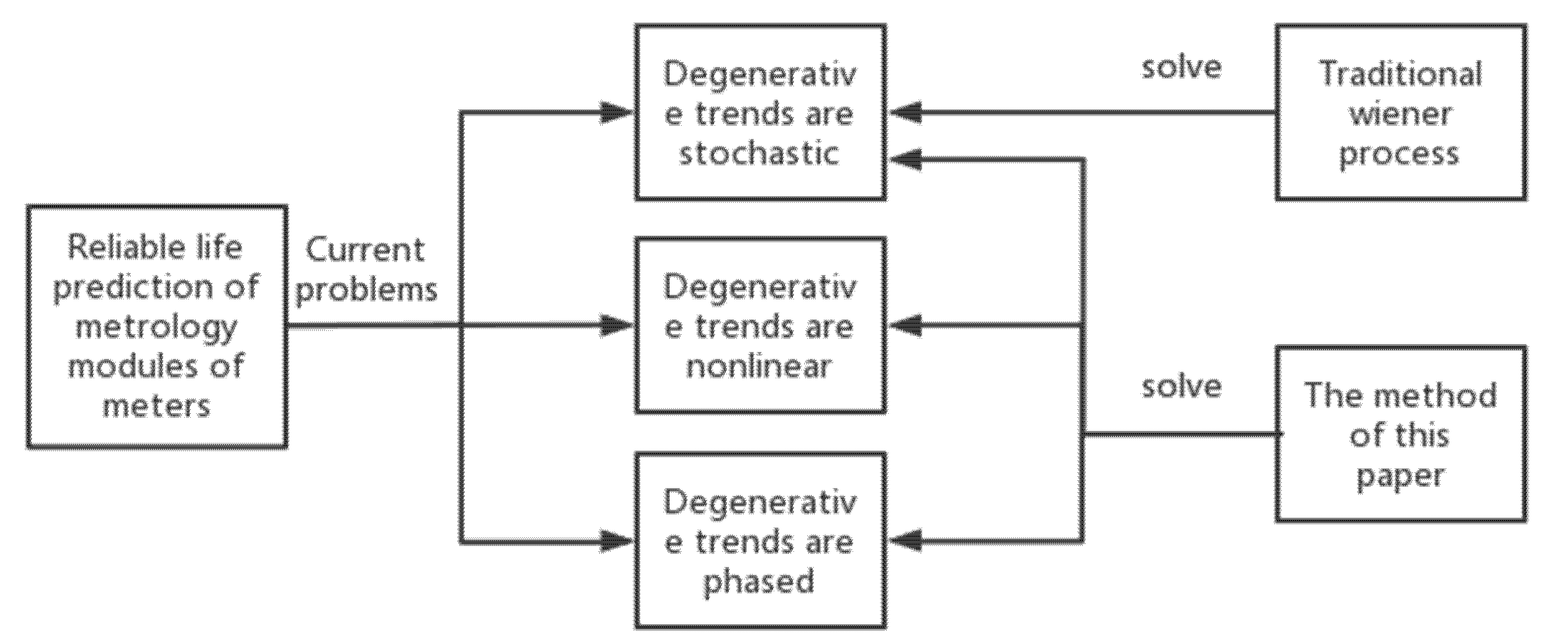
2. Related Work

2.1. Comparison with Traditional Wiener Process Methods

Traditional Wiener process methods are mostly used to describe degenerate processes with stochastic nature. There are two main problems with traditional Wiener process degradation modeling approach if applied to the research object of this paper, expressed graphically in Figure 1.

a.

The modeling does not take into account the nonlinear degradation trend in the modeling object. Since complex electronic products contain a variety of modules, the final degradation trend of the electronic product should theoretically be a combination of the degradation trends of each module. However, in the actual operation [10], within a certain time range, each module degradation starts to accelerate at different time points and degradation speed, so it may cause the randomness and nonlinearity of the final degradation trend of the electronic product.

b.

The model did not take into account whether the modeling object has stage characteristics. For example, capacitors [11], light-emitting [12] diodes, and other electronic products have stage changes in their degradation process, so it is necessary to consider how to deal with the stage characteristics of the degradation trend in the modeling process for the meter that contains these components.

The method used in this paper is a comprehensive and improved approach that makes use of a scale transformation method that linearizes the nonlinear function. The model is partitioned by analyzing the cumulative degradation rate of the target degradation model to ensure that the separated models can better describe the degradation lifetimes of the respective stages to which they belong.

2.2. Application of the Wiener Process Method

In 1995, Pettit [13] proposed applying the Wiener process to build a product life model through simulated data to estimate the product life. The Wiener process is a continuous significant incremental process model. It is fit for stochastic process analysis. It can reveal the performance degradation of multiple typical products [14,15] and consider the differences between pilot production. The Wiener process fully considers the randomness and dynamics of performance degradation in tests [16].

According to the statistics of the State Grid Corporation of China, the failure rate of the measuring module is top among the normal use of the meter. Therefore, this paper selects the reliability of the metrology module as the basis to measure the reliability of the meter. Aiming at the possible nonlinearity in the process of product degradation, Ge et al. [17] combined Wiener process method with a Rul method to establish a nonlinear life prediction model. Based on the nonlinear characteristics in the degradation process of lithium–ion battery, Zhu et al. [18] transformed the nonlinear degradation model into a linear model so that the product degradation process could be modeled by the Wiener process. Yan et al. [19] described a two-stage degradation process with nonlinear time-varying mean and variance and a life degradation model with individual differences in the location of change points.

In summary, without extending the accelerated life test time, combined with the advantages of previous methods, this paper uses the method based on Wiener process to analyze the performance degradation of meters after the accelerated life test. Based on the nonlinear characteristics in the process of measuring the performance degradation of meters and the difficulty with data processing, this paper uses the method of time scale transformation. The possible nonlinear influence during modeling is fully considered to predict the reliability attenuation of meters.

3. Problem Formulation and Methodology

3.1. Data Modeling Based on Wiener Process

Assume the degradation of performance fits the Wiener process, i.e., when the product’s performance degradation function $X\left(t\right)$: $X\left(t\right)-X\left(s\right)\sim N\left(0,t-s\right)$ is valid in $0\le s\le t$ [20], a random process function and an independent increment function in continuous events, then let the standard Brownian motion be $W\left(t\right)$ and

$$X\left(t\right)=\mu t+\sigma W\left(t\right).$$

(1)

where $\mu ,{\sigma }^2$ are positional parameters.

Set $\mathrm{l}$ as the failure threshold of the product.

$$T=inf\left\{t\right|X\left(t\right)\ge l,t\ge 0\}$$

(2)

where T is the inverse Gaussian distribution, [21] and the probability density function is

$$f\left(t\right)=\sqrt{l/\left(2\pi {\sigma }^2{t}^3\right)}{e}^{-{(l-\mu t)}^2/\left(2{\sigma }^{2}t\right)}$$

(3)

Therefore, using Wiener process modeling requires data with the following characteristics:

a.

For any t > 0, the data must obey the normal distribution $N\left(0,{\sigma }^2\right)$;

b.

The data must have independent smooth increments.

3.2. Estimation of Winner Process Parameters

To establish the degradation model, the maximum likelihood method is used to estimate the unknown parameters in Formula (4) for $i$. Assume that the degradation data of the i of the electric meter at the time are $i$. The performance degradation of product i at $i$ is denoted as $\mathsf{\Delta }{x}_i=X_i-X_{i-1}$. According to the Wiener process, $W_i\left(t\right)\sim N\left(0,\mathsf{\Delta }{t}_i\right)$, the performance degradation conforms to the normal distribution [22], i.e.,

$$\mathsf{\Delta }{x}_i\sim N\left(\mu \mathsf{\Delta }{t}_i,{\sigma }^2\mathsf{\Delta }{t}_i\right)$$

(4)

therefore, the probability density function of increment $\mathsf{\Delta }{x}_i$ is

$$f\left(t\right)=\frac{1}{\sqrt{2\pi {\sigma }^2\Delta t_i}}\exp [-\frac{{(\mathsf{\Delta }{x}_i-\mu \mathsf{\Delta }{t}_i)}^2}{2{\sigma }^2\mathsf{\Delta }{t}_i}]$$

(5)

Then the likelihood function of the joint probability density of the degenerate increments is shown the equation:

$$L\left(\mu ,{\sigma }^2\right)={{\displaystyle \prod }}_{i=1}^n \frac{1}{\sqrt{2\pi {\sigma }^2\mathsf{\Delta }{t}_i}}\exp [-\frac{{(\mathsf{\Delta }{x}_i-\mu \mathsf{\Delta }{t}_i)}^2}{2{\sigma }^2\mathsf{\Delta }{t}_i}].$$

(6)

Take the logarithm of Equation (7) and the partial derivatives of $\mu ,\sigma$

$$\left\{\begin{array}{l}\stackrel{\wedge }{\mu }=\left[\frac{1}{n}{\displaystyle {\displaystyle \sum }_{i=1}^n}\frac{\Delta x_i}{\Delta t_i}\right]\\ \stackrel{\wedge }{{\sigma }^2}=\left[\frac{1}{n}{\displaystyle {\displaystyle \sum }_{i=1}^n}\frac{{(\Delta x_i-\lambda t_i)}^2}{\Delta t_i}\right].\end{array}\right.$$

(7)

Through Equation (7), we can calculate the specific value in Formula (4) for $\mu ,\sigma$.

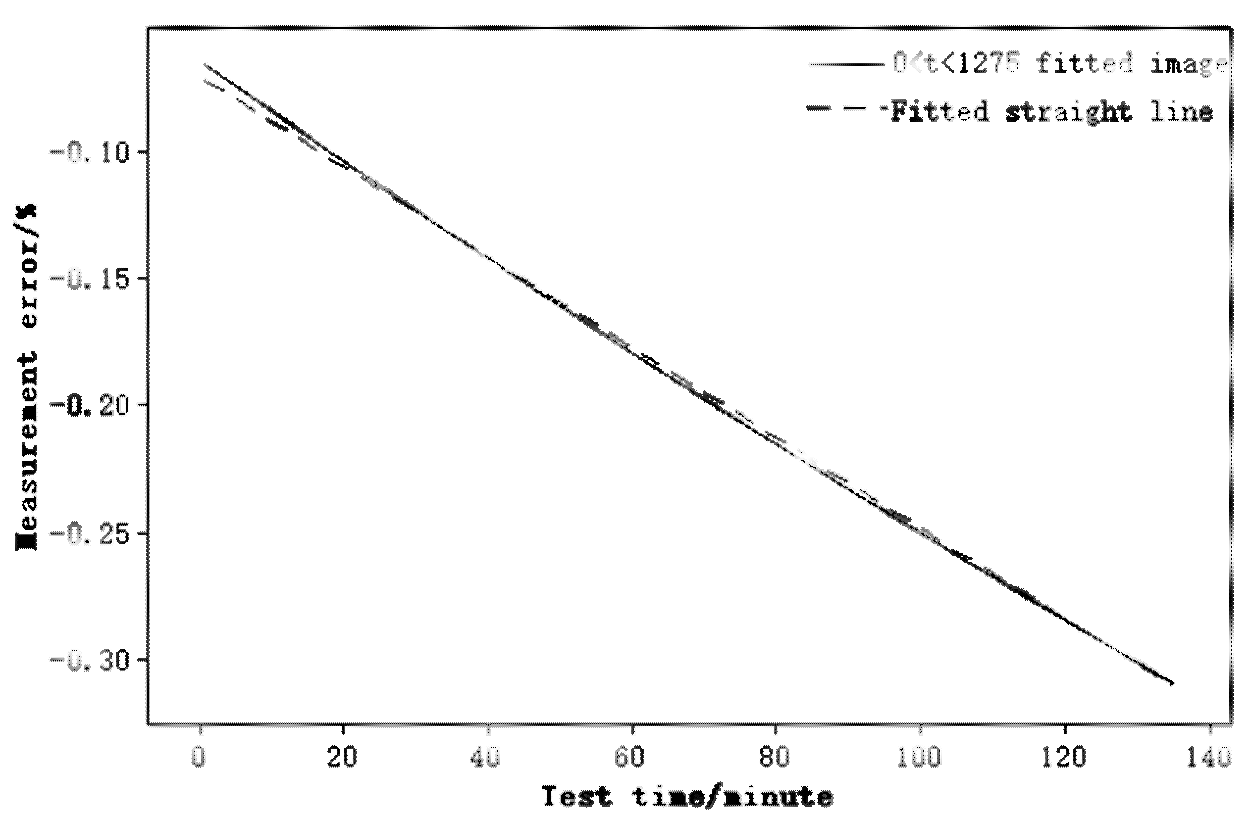
3.3. Linearization of the Nonlinear Model

When the average degradation rate of the product is constant, the performance degradation process can be modeled by Equation (1). However, affected by the environment, the measuring performance degradation of meter presents the characteristics of nonlinearity and randomness, resulting in the degradation rate being not constant.

The power is obtained by multiplying the current obtained by the current sampler and the voltage and current obtained by the voltage sampler, and the measurement error is calculated by the formula:

$$w=\frac{P_{cur}-P_{st}}{P_{st}}\times 100\%$$

(8)

where $P_{cur}$ is the power obtained by multiplying the output of the voltage sampling module and the current sampling module and $P_{st }$ is the power of the standard meter. During the whole life cycle of the meter, if the loss conditions affecting metering performance remain unchanged, the degradation rate is constant. However, in practice, according to Figure 2 of the metrology module, the metrology quality of the metrology chip is affected by the manganin current sampler, the resistance partial voltage sampling circuit and the power supply circuit at the same time. In the high temperature and high humidity test, the thermal shrinkage and cold expansion characteristics of the material affect the performance of each module, so that the degradation speed of the module is faster with the growth of time, and there is a certain randomness in which module will degrade first [23]. Therefore, as a metrology error affected by many factors, it is obvious that the change rate of error is nonlinear and random. In the field, it is quite common that the metrology error is nonlinear and degraded due to the complex environment and external impact. Based on this inference, in this paper, we assume that the metrology error of the meter is nonlinear in the accelerated life test of high temperature and high humidity.

Hence, it needs to be linearized before using Wiener process:

a.

The Wiener model is established in segments and the data $\sigma$ are assumed to be fixed as a whole.

b.

The performance degradation trajectory is obtained, and the fitting equation is calculated.

c.

The coefficients of the time scale transformation function are estimated by using the coefficients of the fitting equation. The time scale change model is used to transform time t, and the nonlinear degradation process is transformed into a linear degradation process.

The time scale transformation model is derived from the performance degradation trajectory to scale the nonlinear data. Suppose that there is a nonnegative monotonic increasing function $\lambda \left(t\right)$ of T, so that $\mu \left(t\right)$=${\mu }^{\prime }\left(t\right)$; then, Equation (1) can be written as

$$X\left(\lambda \left(t\right)\right)=x_0+{\mu }^{\prime }t+\sigma W\left(\lambda \left(t\right)\right)$$

(9)

where ${\mu }^{\prime }$ is the degradation rate after the time scale transformation, and $x_0$ is the initial value of performance degradation.

The time scale transformation model $\tau =\lambda \left(t\right)$ is used to transform T, and $Y\left(\tau \right)=X\left(t\right)$; Equation (5) can be transformed into

$$Y\left(\tau \right)=x_0+{\mu }^{\prime }\tau +\sigma W\left(\tau \right)$$

(10)

Equation (10) is a linearizable nonlinear Wiener process, which can be used to model nonlinear degraded data. When $\lambda \left(t\right)$= t, the linear model can be changed into a univariate linear Wiener degenerate model [24] as a special case of Equation (10).

3.4. Reliability Life Prediction Model of a Meter Based on Nonlinear Data

The measuring performance is the most critical function of the meter, and the meter is a nonrepaired product. The measuring failure implies the scrapping of the meter. Therefore, the correct evaluation of the measuring performance of the meter is very important to evaluate the reliability of the meter.

After building the Wiener degradation model, if the degradation rate of the cumulative metrology error is not constant, but the performance degradation trajectory can be approximated as constant [25] in different stages, the univariate linear Wiener degradation model can be directly established in stages according to Equation (1). Curve fitting is performed for the degradation amount of cumulative metrology error, and a performance degradation model in line with its degradation trajectory is established. R-sq and R-sq (adjust) are selected as the evaluation indices to evaluate the goodness of fit, and the formulas are:

$$R-Sq=\frac{{{\displaystyle \sum }}_{i=1}^n{({{\displaystyle \hat{y}}}_i-\overline{y})}^2}{{{\displaystyle \sum }}_{i=1}^n{(y_i-\overline{y})}^2}$$

(11)

$$R-Sq(adjust)=\frac{\frac{{{\displaystyle \sum }}_{i=1}^n{({\hat{y}}_i-\overline{y})}^2}{n-p}}{\frac{{{\displaystyle \sum }}_{i=1}^n{(y_i-\overline{y})}^2}{n-1}}$$

(12)

where R-sq represents the goodness of fit of the regression equation and is an important parameter to measure whether the regression equation is appropriate. The closer its value is to 1, the better the fitting effect of the regression equation is; R-sq (adjust) is the correlation coefficient deducting the number of included terms in the regression equation. If both R-sq and R-sq (adjust) are close to 1, the smaller the difference between them and the stronger the explanatory ability of the model to variables, where $\widehat{y_i}$ denotes the y value calculated by the fitted equation, $y_i$ is the actual value y, n is the total number of observations, and p is the total number of terms in the regression equation.

Assuming that the degradation trajectory of the degradation amount of cumulative metrology error is T =$\lambda \left(t\right)$, when $\lambda \left(t\right)$= t, the degradation trajectory is a linear Wiener process.

If the model $\lambda \left(n\right)$ is a nonlinear function, there is a formula:

$$t^{*}=\lambda \left(t\right)$$

(13)

The time scale transformation model is used to transform the time scale of the segmented cumulative test time t, the segmented operation times after the time scale transformation are recorded as $t^{*}$, and $Y\left(t\right)=Y\left(t^{*}\right)$. Then, the degradation rate of the cumulative metrology error degradation T on the transformed time scale is approximately constant, which transforms the nonlinear Wiener process into a linear Wiener process.

Then, a model in which the composition of the cumulative metrology error degradation of measuring performance $T\left(t^{*}\right)$ and the cumulative test time after time scale transformation ${\mathrm{t}}^{*}$ conforms to the univariate linear Wiener process.

$$T\left(t^{*}\right)=T(t_0)+{\mu }^{*}{t}^{*}+{\sigma }^{*}B\left(t^{*}\right)$$

(14)

where $T\left(t^{*}\right)$ is the cumulative metrology error;$T(t_0$) is the cumulative metrology error at the initial time;${\mu }^{*}$ is the degradation rate of the cumulative quantity, which represents the average degradation trend of measuring performance degradation; $t^{*}$ is the cumulative test time after time scale model transformation; ${\sigma }^{*}$ is the diffusion velocity of the cumulant, which indicates the influence of random factors, such as test error and external environmental interference on degradation; and $B\left(t^{*}\right)$ is the standard Brownian motion.

Since the linearizable Wiener process will eventually be transformed into a univariate linear Wiener process, the probability density function and reliability function of their residual life are the same. For the linearizable Wiener process, the key is to solve the time scale model of the nonlinear degradation process t* = λ(t). It is proven that under the condition that the average performance degradation rate of the product is constant, the time distribution of the Wiener process reaching the failure threshold for the first time is an inverse Gaussian distribution.

Therefore, under the condition that the failure threshold is L and the average performance degradation rate of the measuring performance of the meter is constant, the probability density function of the remaining life after the transformation of the time scale model is

$$f\left(t*;L\right)=\frac{L-T\left(t_0\right)}{\sqrt{2\pi {({\sigma }^{*})}^3{(T\left(t^{*}\right))}^3}}{e}^{\frac{-\left(L-T_0-{\mu }^{*}T\left(t^{*}\right)\right)}{2{({\sigma }^{*})}^{3}T\left(t^{*}\right)}}$$

(15)

where $f\left(t^{*};L\right)$ is the probability of reaching the failure threshold L in a small range near time ${\mathrm{t}}^{*}$. In general, the expected value of the probability density function can be used as the predicted value of the remaining life of the product [16]. Finally, the actual life of the meter should be expressed by the actual time. It is necessary to carry out the inverse transformation of the time scale model for the predicted value of the remaining life to obtain the predicted value of the actual remaining life, and the actual life of the meter should meet the interval defined in Equation (16).

$$T=inf\{n:T\left(t\right)\ge L\left|T\left(t\right)\le L\right|\}$$

(16)

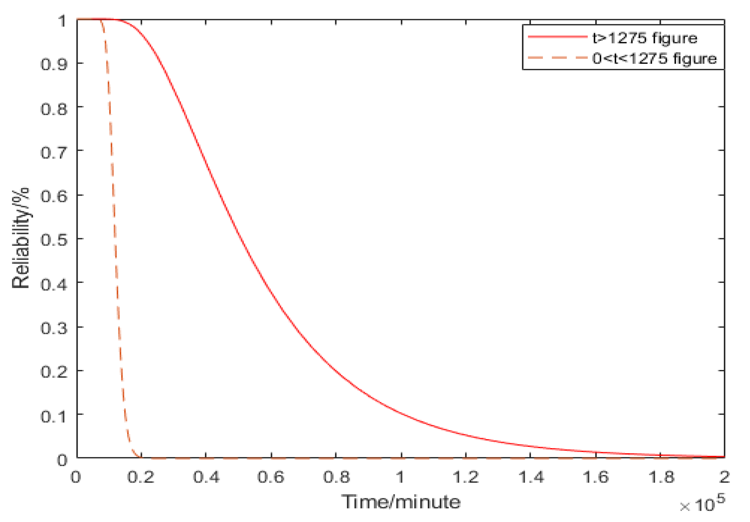
4. Analysis of Results

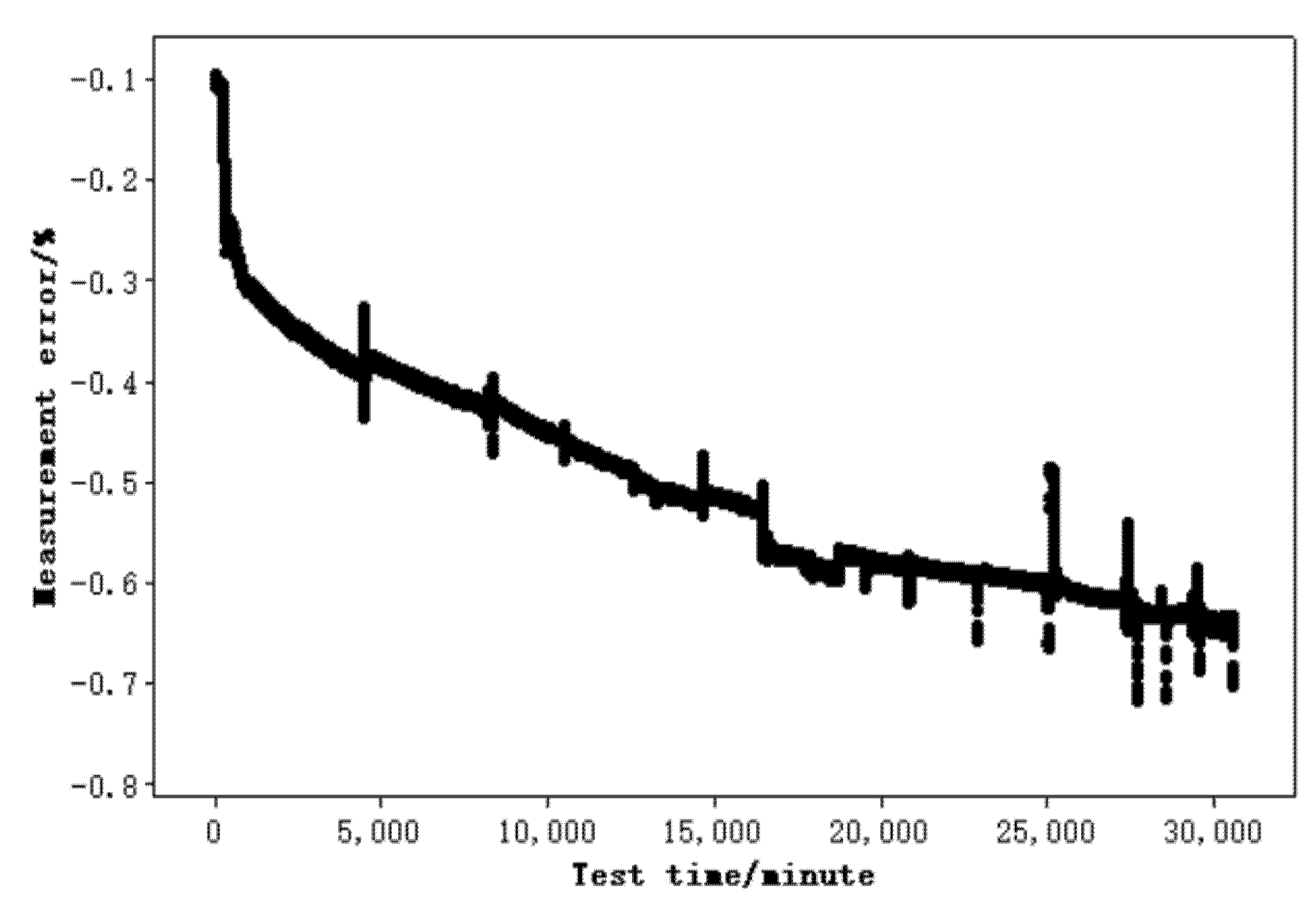
4.1. Experimental Design

This paper uses the accelerated life test method to carry out the test according to method a provided by IEC62059-32-1-2011 Electricity Metering Equipment-Dependability-Part 32-1 and designs the test parameters in

Table 1. Electrical life test parameters.

Parameter	Value
Meter test voltage	Rated voltage of meter
Meter test current	Rated current of meter
Power factor	1
Temperature of environmental test chamber	85 ℃
Humidity of environmental test chamber	95%
Number of test days	30
Number of test tables	30

below. High environmental pressure is applied to the meter through the environmental test chamber to accelerate the change speed of the service life of the meter. The specific flow of the test is shown in Figure 3 below.

During the accelerated life test, the 485 serial port was used to read the pulse signal of the meter every minute and compare it with the signal of the standard pulse source to obtain the measurement error at the current time. Some measurement error data are shown in

Table 2. Degradation of the measurement error of the meter.

Test Time/Minute	Measurement Error/%
	Sample 1	Sample 2	…	Sample 30
0	−0.1013	−0.0917	…	−0.0870
10,000	−0.4557	−0.4848	…	−0.4840
…	…	…	…	…
32,736	−0.6912	−0.7218	…	−0.7315

below. Under high environmental pressure, the performance of the measuring module of the meter is worse. After the accelerated life test, the statistical regression method was used to fit the curve between the measurement error of the meter and the cumulative time of the test.

From the cumulative rate of increase in metrology error in Figure 4 above, it can be seen that there are many differences in the images with x = 1275 as the dividing point, so it is divided into two segments and processed. After smoothing, the curve is refitted. The R-sq of the two piecewise functions is closest to 1 when fitting the second-order function, which shows that the second-order function can best reflect the change relationship between metrology error and time, so it is considered that they are quadratic functions. This result also proves the assumptions in Section 3.3.

Time scales of the two piecewise functions are transformed. Among them, the time scale transformation is performed for the image with 0 < T < 1275, and the transformation effect is shown in Figure 5 and Figure 6. After transformation, the R-sq of the first half increases from 83.5% to 99.9%. R-sq ≈ R-sq (adjust), so it can be judged that the original second-order function model can be approximated to a linear model after the transformation of the time scale.

Similarly, if the fitting equation in the range of t ≥ 1275 is scaled, there is a piecewise probability density.

$$f\left(t\right)=\left\{\begin{array}{l}\frac{l}{\sqrt{2\pi {\sigma }_1{}^2{T}_1^3\left(t\right)}}\exp [-\frac{(l-{\mu }_1{T}_1^2\left(t\right)}{2{\sigma }_1{}^2{T}_1\left(t\right)}](0<t<1275)\\ \frac{l}{\sqrt{2\pi {\sigma }_2^2{T}_2^3\left(t\right)}}\exp [-\frac{(l-{\mu }_2{T}_2^2\left(t\right)}{2{\sigma }_2^2{T}_2\left(t\right)}](t\ge 1275)\end{array}\right.$$

(17)

From Equation (7) and the linear fitting results of the functions at both ends, we can obtain the following

Table 3. Estimation results of parameters in this paper.

Parameter	${\mathsf{\mu }}_1$	${\mathsf{\sigma }}_1^2$	${\mathbf{a}}_1$	${\mathbf{b}}_1$
Value	$1.643\times {10}^{-4}$	$2.134\times {10}^{-5}$	$4.67\times {10}^{-5}$	$2.240\times {10}^{-6}$
Parameter	${\mathsf{\mu }}_2$	${\mathsf{\sigma }}_2^2$	${\mathbf{a}}_2$	${\mathbf{b}}_2$
Value	$3.422\times {10}^{-5}$	$1.692\times {10}^{-5}$	$1.86\times {10}^{-5}$	$1.251\times {10}^{-6}$

.

According to OIML R 46-1/-2, the threshold l is set as the maximum acceptable metrology error ± 0.2% for the meter. The l here corresponds to the l in Equation (17)

$$R\left(t\right)=1-F\left(t\right)$$

(18)

The failure rate F(T) is obtained by integrating Equation (17), the reliability R(T) is obtained by Equation (18), and the reliability function of the meter is drawn in Figure 7.

The calculation shows that the reliability image of the piecewise function coincides within the range of T = 7123 and covers the range of 0 < T < 1275, so it can be used.

$$f\left(t\right)=\frac{l}{\sqrt{2\times {0.00462}^2{t}^3}}\exp [-\frac{{(l-0.00003422\mathrm{t})}^2}{2\times {0.00462}^{2}t}]$$

(19)

Equation (17) can be replaced as the final reliability prediction model formula of meters.

According to the reliability model in the figure, the time for meters to express 91% reliability is 25,240 min. According to the conversion formula of the actual working time in IEC62059-31-1:2008:

$$t_n=t_{\mathrm{ij}}\times AF$$

(20)

where AF is the acceleration factor. According to the accelerated life test parameters designed in this paper, the acceleration factor can be calculated to be 473.23. Therefore, its actual service life is calculated to be 22 years.

4.2. Comparison with Traditional Models

Afterwards, this batch of tested meters is tested until there is a failed sample. Then, the reliability is calculated by the number of failures. The differences between the reliability calculated by the degradation parameters and the previous reliability calculated by the failure number are compared. The reliability function of the original method and the method in this paper is subtracted to obtain the error diagram in Figure 7. The above formula can calculate that when the electric energy is expressed to 91%, the actual life predicted by this method is 22 years, the prediction result of the previous method is 23 years, and the true value result of the actual life is between the two.

Therefore, Figure 8 shows that the reliability calculated by this method is similar to that calculated by conventional methods, which proves the prediction accuracy. Based on this method, the required amount of data to predict the service life of meters is greatly reduced.

4.3. Field data Analysis

Since the meter used in the test is a new one, its on-site use is lesser. To verify the correctness of the model, three meters from the same batch of meters used in the accelerated life test were selected and put into use for a period of time, and their current life after being used in the actual environment for a period of time was calculated using Equation (13) to comparing the estimation accuracy of unprocessed and nonlinear Wiener models in the field use environment. The results are shown in

Table 4. Comparison of model prediction results.

Relative Error of the Unprocessed Model/%	Relative Error of the Nonlinear Model/%
10.273	6.956
−10.377	−5.722
−11.696	−8.637
7.079	3.834
8.510	5.358

.

It can be seen from the table that the nonlinearized model is more accurate than the unprocessed model and closer to the actual service time. The unit of time used in the table is minutes, and after converting it to days, it can be found that the current life predicted by the model differs from the time of use by at most two days, which can be considered negligible in the use of the meter in years as the unit of measure, so the prediction result of the nonlinear model is more desirable.

5. Conclusions

The current meters have high reliability and a nonlinear change law in the process of measuring performance degradation. In this paper, the time scale transformation method was used to convert the nonlinear degradation process into a linear process. Combined with the Wiener process, the maximum likelihood method is used to reckon its unknown parameters. By establishing the degradation model to measure the performance of meters, the method to predict the product life is improved, and reduce the time of the reliability test of the meters and the cost caused by prolonged testing.

The model developed in this paper is mainly applicable to the case where the environmental conditions of the meter vary slightly. If the meter is outdoors and vulnerable to the external environment, which varies greatly, the degradation data of the meter metrology error may be in a complex stochastic state with multi-stage changes. Therefore, the next step will be to further extend the degradation modeling problem with multi-stage complex stochastic variation.

References

- Jaiswal, D.M.; Thakre, M.P. Modeling & Designing of Smart Energy Meter for Smart Grid Applications. Glob. Transit. Proc. 2022, 3, 311–316. [Google Scholar]
- Zhang, X.; Yang, J.; Kong, X. A literature review on planning and analysis of multi-stress accelerated life test for reliability assessment. Recent Pat. Eng. 2021, 15, 12–21. [Google Scholar] [CrossRef]
- Li, Q.; Yan, C.; Chen, G.; Wang, H.; Li, H.; Wu, L. Remaining Useful Life prediction of rolling bearings based on risk assessment and degradation state coefficient. ISA Trans. 2022. [Google Scholar] [CrossRef] [PubMed]
- Wang, F.; Zhao, Z.; Ren, J.; Zhai, Z.; Wang, S.; Chen, X. A transferable lithium-ion battery remaining useful life prediction method from cycle-consistency of degradation trend. J. Power Sources 2022, 521, 230975. [Google Scholar] [CrossRef]
- Al-Bossly, A. Bayesian Statistics Application on Reliability Prediction and Analysis. J. Stat. Appl. Probab. 2020, 9, 19–34. [Google Scholar]
- Ma, L.; Meng, Z.; Teng, Z.; Qiu, W. A reliability evaluation framework for smart meters based on AGG-ARIMA and PFR. Meas. Sci. Technol. 2022, 33, 045006. [Google Scholar] [CrossRef]
- Yang, H.; Wang, P.; An, Y.; Shi, C.; Sun, X.; Wang, K.; Zhang, X.; Wei, T.; Ma, Y. Remaining useful life prediction based on denoising technique and deep neural network for lithium-ion capacitors. eTransportation 2020, 5, 100078. [Google Scholar] [CrossRef]
- Song, K.; Cui, L. A common random effect induced bivariate gamma degradation process with application to remaining useful life prediction. Reliab. Eng. Syst. Saf. 2022, 219, 108200. [Google Scholar] [CrossRef]
- Yan, W.; Kong, W.; Liu, W.; Xiong, Y.; Zhang, J. Reliability assessment of photovoltaic modules with initial degradation random characteristics. Acta Energ. Sol. Sin. 2022, 43, 152. [Google Scholar]
- Dong, X.; Dai, Y.; Wang, Q.; Chen, Z.; Du, Y.; Wang, P.; Qi, J. Reliability Modeling Methods Using Field Operation Data of Smart Electricity Meters Based on Wiener Process. In Proceedings of the 2020 Global Reliability and Prognostics and Health Management (PHM-Shanghai), Shanghai, China, 16–18 October 2020. [Google Scholar]
- Kurzweil, P. Josef Schottenbauer, and Christian Schell. Past, present and future of electrochemical capacitors: Pseudocapacitance, aging mechanisms and service life estimation. J. Energy Storage 2021, 35, 102311. [Google Scholar] [CrossRef]
- Ibrahim, M.S.; Fan, J.; Yung, W.; Jing, Z.; Fan, X.; Driel, W.; Zhang, G. System level reliability assessment for high power light-emitting diode lamp based on a Bayesian network method. Measurement 2021, 176, 109191. [Google Scholar] [CrossRef]
- Fuli, Y.; Ke, Z.; Renmin, G. Reliability prediction method of smart meter based on Hadoop platform and published parameter estimation. In Proceedings of the 2020 5th Asia Conference on Power and Electrical Engineering (ACPEE), Chengdu, China, 4–7 June 2020. [Google Scholar]
- Gao, H.; Cui, L.; Dong, Q. Reliability modeling for a two-phase degradation system with a change point based on a Wiener process. Reliab. Eng. Syst. Saf. 2020, 193, 106601. [Google Scholar] [CrossRef]
- Wang, X.; Hu, C.; Ren, Z.; Xiong, W. Performance degradation modeling and remaining useful life prediction for aero-engine based on nonlinear Wiener process. Acta Aeronaut. Et Astronaut. Sin. 2020, 41, 11. [Google Scholar]
- Sun, F.; Li, H.; Cheng, Y.; Liao, H. Reliability analysis for a system experiencing dependent degradation processes and random shocks based on a nonlinear Wiener process model. Reliab. Eng. Syst. Saf. 2021, 215, 107906. [Google Scholar] [CrossRef]
- Ge, R.; Zhai, Q.; Wang, H.; Huang, Y. Wiener degradation models with scale-mixture normal distributed measurement errors for RUL prediction. Mech. Syst. Signal Process. 2022, 173, 109029. [Google Scholar] [CrossRef]
- Zhu, Y.; Liu, S.; Wei, K.; Zuo, H.; Du, R.; Shu, X. A novel based-performance degradation Wiener process model for real-time reliability evaluation of lithium-ion battery. J. Energy Storage 2022, 50, 104313. [Google Scholar] [CrossRef]
- Yan, B.; Ma, X.; Huang, G.; Zhao, Y. Two-stage physics-based Wiener process models for online RUL prediction in field vibration data. Mech. Syst. Signal Process. 2021, 152, 107378. [Google Scholar] [CrossRef]
- Liao, G.; Yin, H.; Chen, M.; Lin, Z. Remaining useful life prediction for multi-phase deteriorating process based on Wiener process. Reliab. Eng. Syst. Saf. 2021, 207, 10736. [Google Scholar] [CrossRef]
- Bian, L.; Wang, G.; Liu, P. Reliability analysis for multi-component systems with interdependent competing failure processes. Appl. Math. Model. 2021, 94, 446–459. [Google Scholar] [CrossRef]
- Chen, Z. Common fault Analysis and Countermeasures of key Components of intelligent electricity meter. J. Phys. Conf. Ser. 2020, 1654, 012055. [Google Scholar] [CrossRef]
- Si, X.; Li, T.; Zhang, J.; Lei, Y. Nonlinear degradation modeling and prognostics: A Box-Cox transformation perspective. Reliab. Eng. Syst. Saf. 2022, 217, 108120. [Google Scholar] [CrossRef]
- Zhang, H. Two-stage nonlinear Wiener process degradation modeling and reliability analysis. Syst. Eng. Electron. Technol. 2020, 42, 6. [Google Scholar]
- Lin, J.; Liao, G.; Chen, M.; Yin, H. Two-phase degradation modeling and remaining useful life prediction using nonlinear wiener process. Comput. Ind. Eng. 2021, 160, 107533. [Google Scholar] [CrossRef]