Cutting Simulation in Unity 3D Using Position Based Dynamics with Various Refinement Levels

Abstract

Augmented and Virtual Reality-based surgical simulations have become some of the fastest-developing areas, due to the recent technological advances and changes, in surgical education. Cutting simulation is a crucial part of the virtual surgery simulation in which an incision operation is performed. It is a complex process that includes three main tasks: soft body simulation, collision detection and handling, and topological deformation of the soft body. In this paper, considering the content developer’s convenience, the deformable object simulation, using position-based dynamics (PBD), was applied in the Unity 3D environment. The proposed algorithm for fast collision detection and handling between the cutting tool and the deformable object uses a sweep surface. In case of incision, the algorithm updates the mesh topology by deleting intersected triangles, re-triangulation, and refinement. In the refinement part, the boundary edges threshold was used to match the resolution of new triangles to the existing mesh triangles. Additionally, current research is focused on triangle surface meshes, which help to reduce the computational costs of the topology modifications. It was found that the algorithm can successfully handle arbitrary cuts, keeping the framerate within interactive and, in some cases, in the real-time.

1. Introduction

Virtual simulation is a reproduction of a real-world environment obtained with the help of a computer system, which allows user to interact with the simulated objects. Nowadays, due to the progress in computational science, virtual simulation became a rapidly growing area. Virtual simulation is used in many different fields, such as engineering, education, natural sciences, medicine, and so on. Many scientific papers were dedicated to study how the virtual simulation impacts education and teaching. Researchers in [1] provide information on a web-based simulation platform named EDISON, which can be used to simulate different physical phenomena. Ref. [2] proposes a Mixed Reality Chemistry Lab to simulate chemistry experiments and help students to obtain needed knowledge before starting to work with actual chemicals. The research in [3] summarizes the most important features of virtual simulations in education, such as visualization, inclusiveness, unlimited access to information, and increased engagement. Ref. [4] examines the application of virtual simulations in higher education. The study concludes that VR is a promising technology, and it is often used to obtain skills, which require declarative knowledge and procedural–practical knowledge. Nonetheless, there are proofs that AR and VR technologies are highly suitable in medicine, and there are many different applications of it in treatment and rehabilitation. Research in [5] effectively uses VR simulation in rehabilitation purposes to cure vertigo conditions. Ref. [6] proposes VR-based exposure therapy to treat mental illness. The research shows promising results and proves that plausible VR images can replace expensive on-site hardware. Therefore, virtual simulation is expected to be successfully applied in the medical sphere and education. Combining the two areas of study, there are certain proofs of AR and VR being useful in medical education and, especially, in surgery training.

Surgery is a complicated process, and in order to be successfully executed, it requires a certain amount of practical skills from a surgeon. Traditional surgeon education includes operating room (OR) assistance, surgery observation outside of OR, and different types of simulation models, such as bench-top and laparoscopic box simulators, manikins, live animals, human cadavers, virtual reality (VR), and others [7]. However, it takes a great deal of time to acquire the needed motor skills before a trainee can become a surgeon. Furthermore, when the trainee imitates the mentor’s actions, one should rely, mainly, on subjective assessments [8]. Additionally, during OR assistance, there is a risk of accidentally making a medical error, which would harm a patient or even the surgeon. Ref. [9] relates the high frequency of surgical errors to the inexpertness of surgeons. The researchers presume that appropriate education and improvement of diagnostic and therapeutic skills can help to prevent most of the medical errors. The study conducted in [10] found that surgery and medical procedure-induced adverse events are one of the main reasons for a prolonged hospitalization period, and they may cause significant harm to patients. Therefore, recently, many simulation models were developed to reduce patient involvement at the time of surgeon training. Constant research of simulation-based education is done to find its efficiency. Ref. [7] found that recent surgery simulators provide more collaborative, realistic, and versatile results through the usage of modern technologies, such as VR, 3D printing, and internet connection. The research also emphasizes that the new simulation methods can be used not only in surgeon training but in preoperative planning as well. Ref. [11] states that surgery simulations provide a convenient and nurturing environment for the trainee, while the educator can objectively estimate one’s performance. Ref. [12] showed, that surgical simulations methods, such as VR, porcine model, and box trainer can help to improve the OR performance and operating time of trainees. Among the abovementioned surgery simulation techniques, VR/AR simulation is a promising method. Ref. [11] states that VR/AR simulations provide immersive and repetitive training environment with the advantage of interactive feedback and user’s performance assessment. The clinical trial of 18 orthopedic surgery residents in [13] shows that immersive VR education significantly improves surgical knowledge and procedural metrics. The study also reveals that 1 h of immersive VR training is estimated as 48 min of real-world training time. Thus, VR/AR surgery simulations make it possible to obtain objective and standardized surgical knowledge, while providing safe and plausible educational environment.

Frequently, surgeries require the surgeon to execute a cutting of soft tissues. However, a virtual cut simulation is a complicated process, which involves update of the computational model of an organ and continuous collision detection and handling [14,15]. There are many methods to implement virtual cutting in computer systems, which are mainly categorized by geometrical representations of organs and a numerical discretization model [14,15]. Geometrically cutting simulation approaches are divided into mesh-based and meshless types. Mesh-based methods can be represented by triangle surface, tetrahedral, hexahedral, and polyhedral meshes. In these types of simulations, cutting involves constant topology updates, which can lead to huge computational costs. Meshless or mesh-free approaches usually are represented by points, which are controlled by declared rules of elasticity [14]. For numerical discretization there are many different methods to implement the physical part of simulation, however, the most of researches exploit following three approaches: mass-spring model (MSM), finite element model (FEM), and position-based dynamics (PBD). MSM is a simple and fast simulation model, which was introduced in [16] for simulating deformable objects. MSM discretizes an object into mass-points, and to imitate real-world elasticity, it applies spring forces between the points. Despite MSM’s simplicity and low computational costs, it is hard to tune the model’s parameters to obtain certain visual effects, while the whole system can easily lose its stability, which may induce blow-ups. The next physical model is FEM, which discretizes objects into smaller elements and applies governing differential equations to them [17]. Due to its precise simulation results, FEM is often used in physical phenomena analysis and engineering. However, the results of a FEM-based simulation are highly dependent on the chosen mathematical model, and to achieve higher accuracy the approach may require more refined mesh with bigger number of elements. Therefore, in many cases, because of high computational costs, FEM produces simulations in interactive framerate or offline mode [14]. The last numerical discretization model is PBD, which has the main feature of directly manipulating positions during the simulation [18]. The positions are controlled by applying restraining forces in the form of constraints. The most generally used constraints types are stretching and bending ones. The further discussion on PBD-based simulations will proceed in the Methodology part of the current article.

Active research on the cutting simulation is done based on the abovementioned geometry representation and numerical discretization models. The research in [19] proposed a tetrahedral volume mesh-based interactive cutting simulation, which exploits the look-up table in topology update and avoids cracks during tetrahedron subdivision. Additionally, the researchers used the axis-aligned bounding box technique to enhance collision detection between the cutting tool and the mesh. In [20], the researchers simulated an esophagus by using surface triangular mesh and the boundary element method. Here, a new approach was proposed in which binary tree is used to create a hierarchical database of triangles and trace each triangle subdivision. Ref. [21] designed an extended PBD(XPBD)-based hybrid cutting simulation. In the research, the refined surface triangular mesh is combined with coarser tetrahedral interior mesh to improve the performance of the simulation. Ref. [22] proposes an interesting solution to simulate the cutting and tearing of soft bodies in AR. The authors utilize a spatio-temporal registration technique to capture the deformation of tracked objects and apply it to the computational FEM model. In [23], the researchers proposed an adaptive octree mesh model with embedded structures to simulate the cutting of human organs with nerves and vessels inside them. Ref. [24] used PBD to execute a simulation of electrosurgery on a mesh-free model. The researchers proposed a heat-response threshold to make the cutting process more plausible. Additionally, the framework was able to simulate several human organs in the same scene in real time. In [25], a new hybrid method is proposed, which combines surface mesh and internal meshless point elements through the usage of virtual points. The algorithm simulates cutting in two steps: first, constructing the Bezier curve according to surface collision detection; second, calculating the deformation displacement for the point elements. Ref. [26] proposes a Mass Spring-based three-stage cutting simulation, which includes creation of a swept volume, composition of Bezier curve and retriangulation by using shortest distance node matching algorithm. Additionally, the proposed method calculates residual stress, which helps to simulate tissue shrinking during the cutting.

The current study is focused on the designing of a new method to simulate cutting during virtual surgery simulation basing on PBD. The numerical discretization model was chosen considering instability of MSM and high computational costs of FEM approaches. Additionally, compared to the simulation approaches in [21], the current model is applied only to the surface triangle mesh of the simulated soft body. We intentionally avoid using tetrahedral mesh or other volumetric geometry representation in order to reduce computational costs and achieve cutting simulation in real-time. Furthermore, current research proposes a method to patch and refine large holes, which may appear during cutting. Here, we apply the algorithm from [27], which achieves hole patching using the ear-clipping approach. The refinement level may be set to original surface mesh, with coarser or more refine triangulation depending on user input.

The remainder of this paper is organized as follows. Section 2 explains the overall methodology of the proposed cutting simulation. Section 3 shows the cutting experiments. Section 4 contains the performance evaluation data, and the last section summarizes the main findings of the current research, its limitations, and future works.

2. Methodology

The main parts of the proposed cutting simulation method include composition of PBD model, intersection check, hole patching, and refinement. These steps are described in the following subsections.

2.1. Composition of PBD Model

In current research, PBD is used to physically simulate soft bodies during virtual cutting. Comparing it to many classical force-based approaches PBD influences positions directly, which helps to avoid overshooting and energy loss [18]. Hence, this method can achieve fast, stable, and rather accurate simulation both of rigid and soft bodies. A PBD model consists of N number of particles and M constraints. By tuning the stiffness value k of each constraint, we can adjust elasticity of simulated bodies and achieve different visual effects. The algorithm of PBD is described in Algorithm 1. Here, after receiving the initial positions x, velocities v, and inverted masses w of each vertex, the system solves Euler integration in lines 5–8 to obtain temporal positions p. After that, in line 9, the algorithm iteratively resolves all constraints in a Gauss Seidel-like manner to adjust the predicted positions p. Finally, in lines 10–14, velocity v and position x of all vertices are set based on corrected temporal positions p. To achieve the plausible simulation of soft bodies, two types of constraints were applied: stretching and bending. More information about these constraints can be found in [18].

Algorithm 1. PBD

1: Require: initial positions x 2: Require: initial velocities v 3: Require: initial inverted masses w 4: while simulation is running 5:           for all vertices i do 6:                    vi ← vi + wife(xi)∆t 7:                    pi ← xi + vi∆t 8:           end for 9:           for n times solveConstraints() 10:         for all vertices i do 11:                  vi ← (pi − xi)/∆t 12:                  xi ← pi 13:         end for 14: end while

2.2. Cutting Simulation

The proposed cutting simulation method is shown in Algorithm 2. The cutting starts with the intersection check between mesh triangles and a cutting tool in line 5. Lines 6–12 describe the procedures taken in case of intersection. Firstly, we create a set of intersected triangles and a set of intersected edges. Then, the intersection points are calculated, and intersected triangles are removed from the initial surface mesh. After that, in line 14, to maintain the physical part of the simulation accurately, the algorithm removes constraints corresponding to the edges of deleted triangles. More details on constraint deletion can be found in Appendix A Algorithm A1. Then, in lines 15–16, we define the cutting plane by calculating plane’s normal n_cp. The cutting plane is required to divide all intersected edges into two groups: ones that lie on the positive side of the plane, and ones on the negative side (lines 17–19). The deletion of intersected triangles produces a hole in the mesh with uneven boundaries. Therefore, the next step in the cutting algorithm is to reconstruct the boundary edges of the hole. For the beginning, we delete intersection points which lie too close to each other in lines 20–25. This helps to avoid degenerate triangles in further steps. After adding intersection points to the vertices list, the algorithm creates new boundary for positive side edges in line 27. Then basing on the updated boundary edges, the hole is patched with initial triangles. The triangulation technique is described in Appendix A Algorithm A2. However, to match the original triangles’ resolution, we propose to further refine triangles in line 29. Additionally, we provide options to change the refinement level from coarse to fine based on user input. Finally, the algorithm adds new triangles from line 29 to the surface mesh. Then, lines 28–30 are repeated to triangulate negative side edges too.

Algorithm 2. Cutting Algorithm

1: Require: initial surface triangles t 2: Require: initial vertices v 3: while simulation is running 4:           for all triangles ti do 5:                    checkForIntersections() 6:                    if(intersection occurs) 7:                            add ti to the intersectedTrianglesList 8:                            add edges e1, e2, e3 of triangle ti to the intersectedEdgesList 9:                            find intersection points pint 10:                           remove ti from initial triangle set 11:                   end if 12:          end for 13:          if(intersectedTrianglesList is not empty) 14:                   removeConstraints() 15:                   define cutting plane cp by plane normal ncp and point on the plane xcp: 16:                           ncp ← ecp1 x ecp2 17:                   for all edges eii in intersectedEdgesList do 18:                           if(eii is on the positive side of plane cp) add eii to the positiveEdgesList 19:                           else add eii to the negativeEdgesList 20:                   for all intersection points pinti do 21:                           for all intersection points pintj do 22:                                   if((||pinti − pintj ||) < minDistance) pintn ← pintj 23:                           end for 24:                           if((||pinti − pintn|| < α) remove pintn from intersection points list 25:                   end for 26:                   add intersection points pint to the list of vertices v 27:                   positiveEdgesList ← createNewBoundary(positiveEdgesList) 28:                   patchTrianglesList ← triangulate(positiveEdgesList) 29:                   refinedTrianglesList ← refine(patchTrianglesList) 30:                   add refinedTrianglesList to the surface triangles list 31:                   repeat steps 27–30 for the negativeEdgesList 32:          end if 33: end while

In current research, we use sweep plane to track the cutting occurrences. The sweep plane is constructed as pictured in Figure 1. The dissecting part of the cutting tool is represented as cutting edge, which is shown in red in Figure 1b. By tracing the position of cutting edge in previous and current frames, we can find the sweep area and define the final sweep plane. The sweep plane is represented by two triangles, as in Figure 1c, which are used to detect triangle–edge intersections with element edges of surface mesh.

As it was mentioned above, after deleting the intersected triangles, there is a hole left in the surface mesh, which requires further patching. However, the boundary edges form an uneven shape, which can cause crenelations during triangulation and unplausible cutting effects. Therefore, in this study we propose a method described in Algorithm 3 to reconstruct boundaries to achieve smooth and fair cutting. The method consists of two steps: first, connect current boundary edges with the closest intersection points (Figure 2c); second, triangulate edges, which form an acute angle (Figure 2d). In the first stage, the algorithm receives one of the edge sets defined in Algorithm 2 lines 17–19, and for each edge e_i, it calculates its center point c, and distances from each edge e_i vertex to the cutting plane (lines 6–8). Next, in line 9, we test whether distance from edge vertices to the plane is more than threshold β. On the occasion of opposite current edge is skipped, assuming that it is close enough to the cutting plane and will not provide distortion during triangulation. Whenever all vertices of edge e_i lie far from the plane, the algorithm iterates through intersection points in lines 10–13 to find the closest point pint_n. After that, a new triangle is created by triangulating vertices of edge e_i and closest point pint_n. The new edges are created and added into boundary edges list and current edge e_i is deleted (lines 15–17).

Yet, after executing lines 5–19 there might be duplicated edges in current boundary edge list. Hence, in lines 20–24 we remove all duplicates to proceed to the second part of the Algorithm 3. The edges should also be sorted for further hole patching as shown in lines 25–31. Finally, the algorithm iterates through a list of sorted edges and calculates the angle between current edge es_i and next edge es_i+1 in line 34. In case of positive acute angle, we create a new triangle from current edge es_i vertices and end vertex of the next edge es_i+1 as in line 36. A new edge e_new is formed from start vertex of edge es_i, and end vertex of edge es_i+1. e_new is further added to the boundary. In case of insufficient angle, no new triangle is created, and the current edge is added to the boundary edges list in line 38. In the end of Algorithm 3, a complete even boundary is created, as it can be seen in Figure 2d.

Algorithm 3. Create New Boundary

1: Require: set of initial boundary edges e 2: Require: set of initial triangles t 3: Require: cutting plane cp 4: Require: set of intersection points pint 5. for all edges ei do 6:          calculate center point c of ei: c ← (startPointei − endPointei)/2 7:          calculate distance dist1 from startPointei to the plane cp 8:          calculate distance dist2 from endPointei to the plane cp 9:          if(dist1 > β and dist2 > β) 10:                   for all intersection points pintj do 11:                           dist3 ← || pintj − c || 12:                           if(dist3 < minDist) pintn ← pintj 13:                   end for 14:                   add new triangle tnew with vertices startPointei, endPointei and pintn to the triangle list 15:                   add new edge enew1 with vertices endPointei and pintn 16:                   add new edge enew2 with vertices pintn and startPointei 17:                   remove ei from the boundary edge list 18:         end if 19: end for 20: for all edges ei do 21:         for all edges ej do if(ei is equal to ej) remove ei and ej 22: end for 23: add e0 from boundary edge list to the sortedList 24: for(i = 0; i < boundary edges number − 1; i++) 25:         ecur ← sortedList[i] 26:         for all edges ej do if(endPointecur is equal to startPointej) add ej to the sortedList 27: end for 28: remove all edges from boundary edge list 29: for all edges esi in sortedList do 30:         calculate signed angle γ between esi and esi+1 31:         if(γ > 0 and γ < 1200) 32:                   add new triangle tnew with vertices startPointesi, endPointesi+1 and endPointesi to the triangle list 33:                   add new edge enew with vertices startPointesi and endPointesi+1 34:         else add esi to the boundary edge list 35: end for 36: return boundary edges list

In current research, we propose to refine initial patch triangulation as it is described in Algorithm 4. Here, we use dictionary structure edgeDictionary, where edges are keys and triangles’ indices are values. The dictionary contains only interior edges of patch triangulation and adjacent triangles’ information, which is used during the swapping procedure. Figure 3 shows the main steps of the refinement approach: firstly, it receives initial patch triangulation as in Figure 3b and, then, the method subdivides triangles, as in Figure 3c, and swaps edges to obtain final triangulation, as presented in Figure 3d. However, before starting subdivision, the pre-refinement edge swapping is performed in lines 6–7. The experimental findings showed that this technique helps to achieve more accurate and balanced triangulation. Figure 3e depicts the triangulation without pre-refinement edge swapping. It is clear to see that, without additional edge swapping, the triangulation is not fair and even, and there is a big difference between the smallest and the largest triangles.

Algorithm 4. Refine

1: Require: set of initial boundary edges e 2: Require: set of patch triangles patchTrianglesList 3: Require: set of initial vertices v 4: Require: edgeDictionary 5: Require: threshold α 6: for all edges edi in edgeDictionary keys do swap(edi) 7: for (l = 0; l < n; l++) 8:          for (i = 0; i < patch triangles number − 2; i++) 9:                    let edge1, edge2, edge3 be the vertices of triangle tpi 10:                   find average length of edges of triangle tpi: curLength ← (edge1 + edge2 + edge3)/3 11:                   if(curLength >α) 12:                           let v1, v2, v3 be the vertices of triangle tpi 13:                           calculate center point of triangle tpi: vc ← (v1 + v2 + v3)/3 14:                           add vc to the vertices list 15:                           substitute triangle tpi with new triangle tpnew1: v1, v2, vc 16:                           add new triangle tpnew2: vc, v2, v3 17:                           add new triangle tpnew3: v1, vc, v3 18:                           if(edgeDictionary contains key edge2) substitute index of tpi with tpnew2 19:                           if(edgeDictionary contains key edge3) substitute index of tpi with tpnew3 20:                           add new key ed1 to edgeDictionary with triangles tpi and tpnew3 21:                           add new key ed2 to edgeDictionary with triangles tpi and tpnew2 22:                           add new key ed3 to edgeDictionary with triangles tpnew2 and tpnew3 23:                   end if 24:         end for 25:         for all edges edi in edgeDictionary keys do swap(edi) 26: end for 27: return patchTrianglesList

After pre-refinement edge swapping, the algorithm proceeds with triangles subdivision in lines 9–25. It calculates average edge length curLength for triangle tp_i in patch triangulation. In case of the curLength is bigger than threshold α, the triangle tp_i will be subdivided. Here 1-to-3 triangle subdivision is executed through division of triangle tp_i into 3 new triangles. For that the center point vc is calculated in line 14. In case of subdivision triangle information in edgeDictionary must be updated the corresponding edges. The edges of new triangles should also be entered into edgeDictionary as in lines 21–23. Finally, the algorithm iterates over all interior edges and swaps them one by one to achieve Delaunay-like fair triangulation. The detailed explanation on swapping algorithm can be found in Appendix A Algorithm A3. As it can be seen in line 7, the subdivision and swapping are repeated for n times. Experiments showed that different models and refinement resolutions may require more or less iterations to achieve better triangulation results. In Algorithm 4, we introduced threshold α to match triangle resolution to the original one of the surface mesh. To find threshold α, firstly, the average boundary edge length t should be calculated as in Formula (1). Here, be_i is a boundary edge. Next, α is obtained through the multiplication of average boundary edge length t with a value z, as in Formula (2). The value z is a user-defined input, which helps to manipulate the refinement level. In current research, we set five such levels: original, 2 times coarser, 1.5 times coarse, 2 times more refine, 1.5 time more refine. The examples of each refinement resolution are shown in Figure 4.

$$t=\frac{1}{n}{{\displaystyle \sum }}_{i=0}^n\left|\left|b{e}_i\right|\right|,$$

(1)

α = tz

(2)

3. Virtual Cut Simulation Using PBD Model

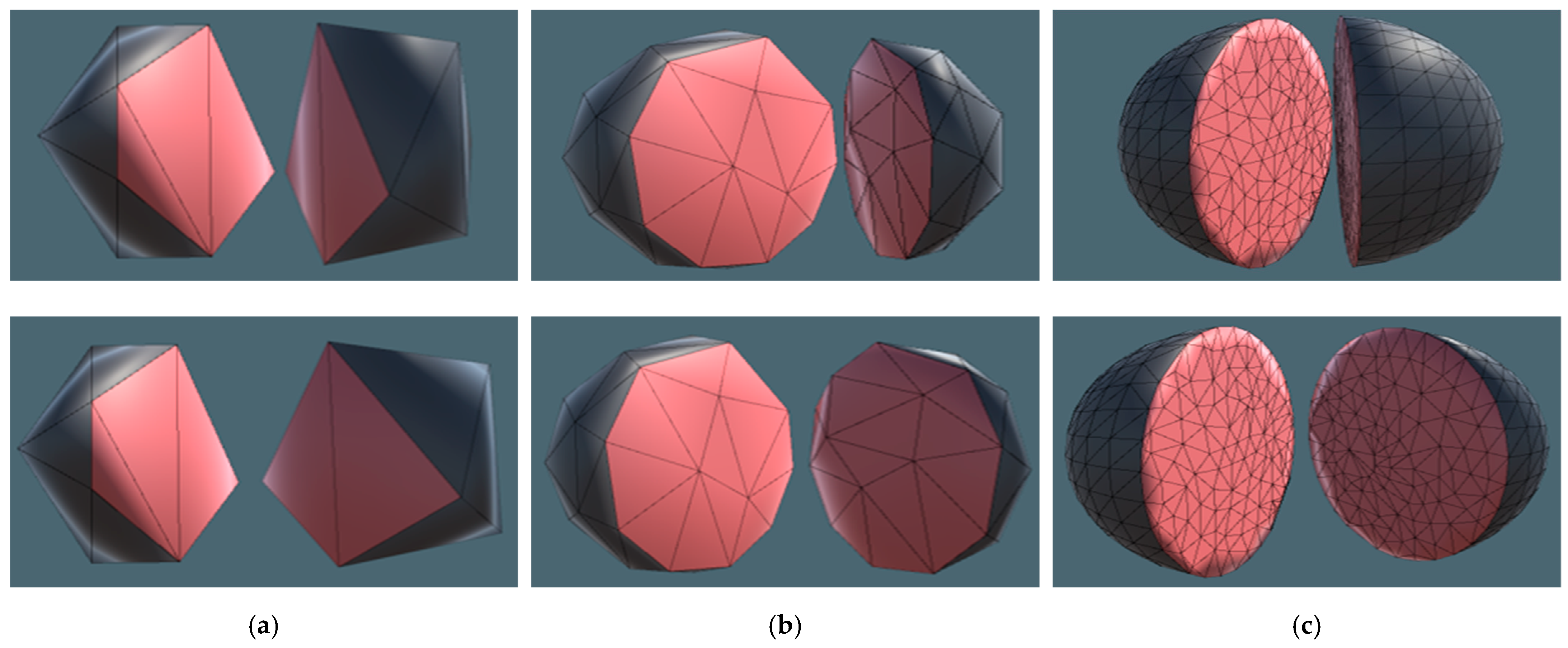
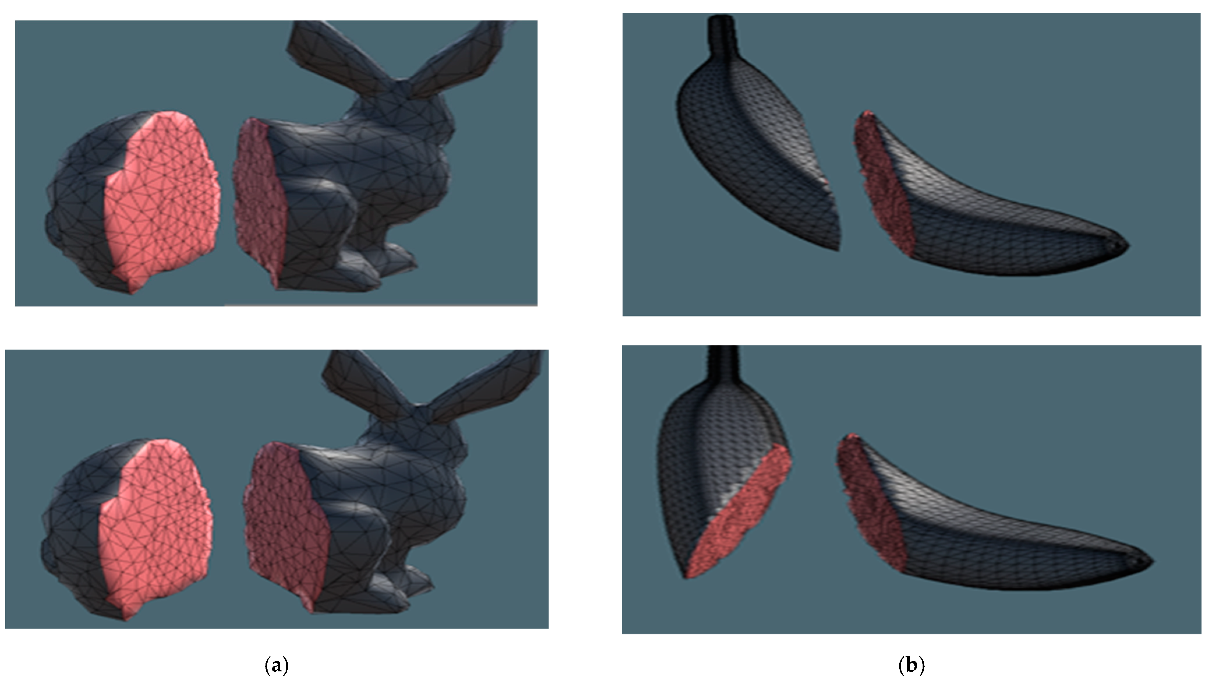
In the current section the information on cutting simulation experiments is provided. The experiment environment consisted of Intel i7-7700 3.60 GHz CPU with 8 cores, GeForce RTX 2080 SUPER GPU, 32 GB RAM and 11 GB V-RAM. The development and tests were executed in Unity 3D game engine version 2019.2.12f1 and Visual Studio 2019 IDE Community edition. In the current study, the PBD part of simulation was executed using GPGPU parallel processing; however, the cutting simulation was implemented purely on CPU. For the experiments we use 7 models: Sphere20, Sphere80, Sphere 768, Bunny, Octopus, Banana, and Armadillo. The smallest model in the test consists only of 20 triangles, and the largest one has over 30,000 triangles.

3.1. Slicing Test

PBD was applied to all experimental models to simulate correct physical behavior. In the current experiment the models were cut with a large sweep plane, which divided them into two parts. According to Algorithm 2, we executed hole patching after deleting the intersected triangles. The initial triangulation was further refined using the Algorithm 4 in order to match the patch triangulation with the original surface mesh.

Figure 5 and Figure 6 show the results of slicing test. In Figure 5, we provide the cutting simulation of simple models: Sphere20, Sphere80, and Sphere768. Figure 6 presents the cutting results of more complex models, such as Bunny and Banana. In all cases, the algorithm provided fair and even triangulation matched to the original resolution. In the case of Sphere20 and Sphere80, the triangle subdivision and swapping were finished in 2-3 iterations. However, for bigger models it required more than 3 iterations of refinement to achieve the best results.

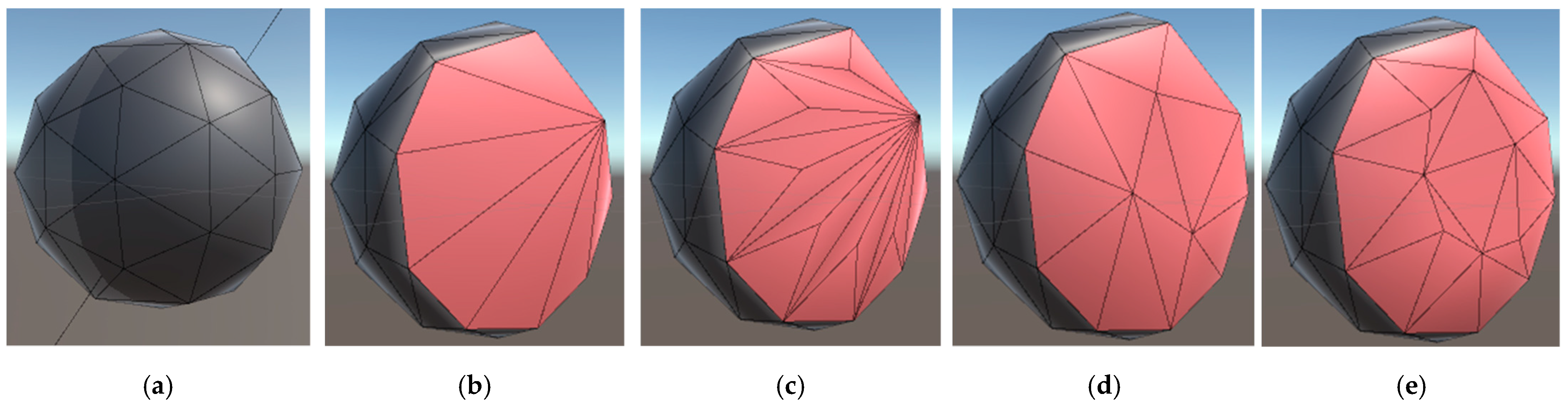
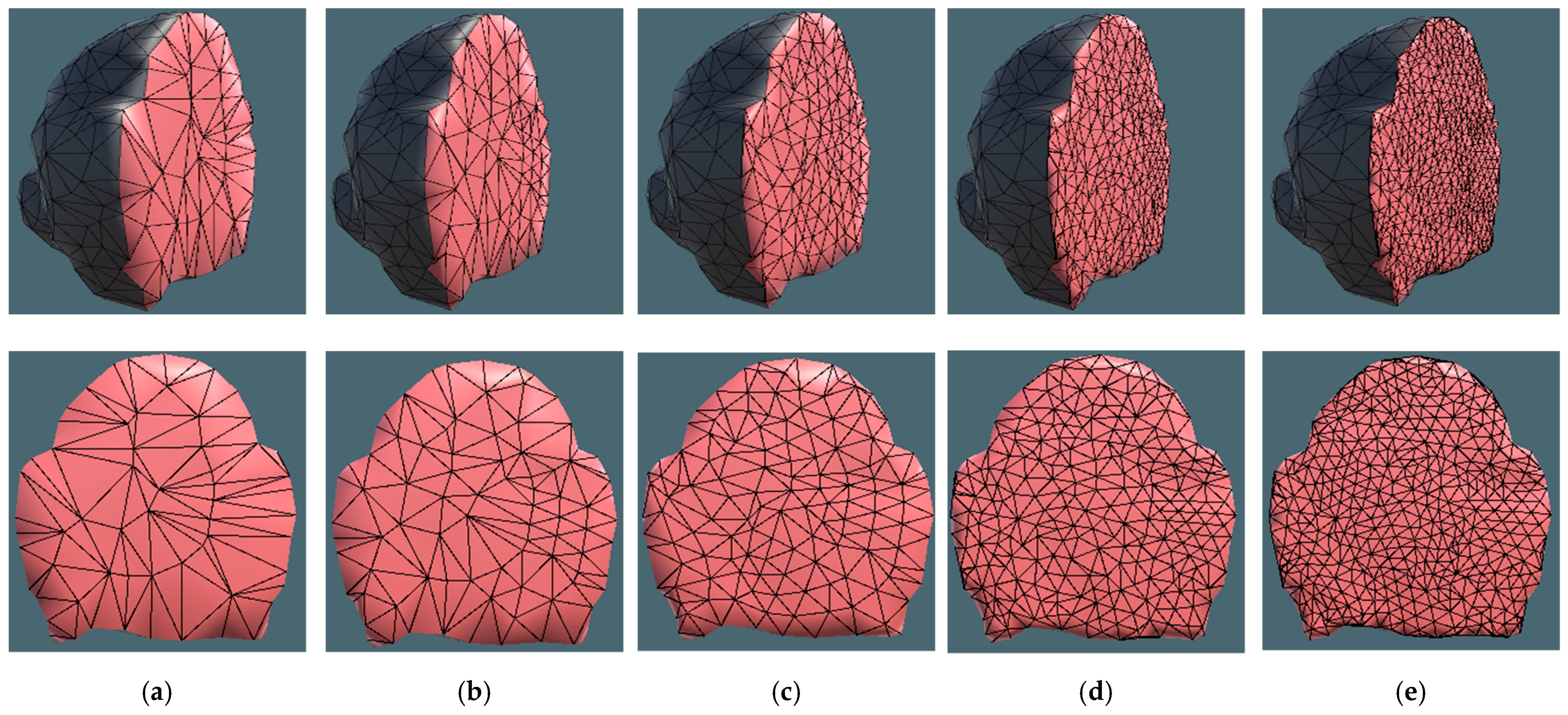
3.2. Refinement Level Test

In the current section we present the refinement test results. As it was mentioned in Section 2.2, the Algorithm 4 proposes five options of refinement level, which can be controlled through the user input.

Figure 7 and Figure 8 show different refinement levels of simple models Sphere20 and Sphere 768. Figure 9 and Figure 10 provide cutting simulation results for more complicated Bunny model. In case of the smallest model, Sphere20, the 2 times coarser, 1.5 times coarser, and original refinement resolutions produce the same results in topology update. The reason for such behavior is that the model is too small to accommodate triangles with larger edges. In other cases, the refinement algorithm provides fair and even triangulation, which corresponds to the original resolution of surface mesh triangles. In Figure 7, Figure 8, Figure 9 and Figure 10, the second parts of the models were intentionally deleted to show, in detail, the refinement levels.

Overall, the proposed solution can handle different kinds of holes and produces satisfactory refinement results. In Figure 10, it can be observed that the hole patching and refinement algorithm manages even thin difficult shapes, such as the ear part on the bunny model. The results of cutting simulation for other models can be found in Appendix A, Figure A1, Figure A2, Figure A3 and Figure A4.

4. Results

To evaluate the proposed algorithm, firstly, we compared frames per second (FPS) rate of only PBD simulation of soft body and the case of PBD with cutting simulation (CS). The FPS measurements of the seven test models are presented in Figure 11. Here, the y axis stands for the FPS rate, and the x axis represents the time of simulation in seconds. In both cases first 15 s of simulation were evaluated.

Table 1. Average FPS comparison.

Model	Number of Vertices	Number of Triangles	PBD avr. FPS	PBD + CS avr. FPS	FPS Difference (%)	Avr. Cutting Time in ms
Sphere20	60	20	231.8	205.9	25.9 (11.17)	11.33
Sphere80	240	80	231.3	177.2	54.1 (23.39)	12.66
Sphere768	515	768	158.6	108.4	50.2 (31.65)	21.66
Bunny	752	1500	135.6	79.9	55.7 (41.08)	29.33
Octopus	1939	2816	103.2	51.7	51.5 (49.9)	38
Banana	2894	5592	72.9	32.1	40.8 (55.97)	80
Armadillo	18,992	30,000	9.9	5.2	4.7 (47.47)	239.33

describes average FPS for PBD only case and PBD with cutting simulation for all 7 test models. Additionally, in Table 1 we show the FPS difference between the two cases. The results from Figure 11 and Table 1 reveal that, in case of only PBD, as well as in PBD with the cutting simulation all models, except for Armadillo, real-time FPS rate is achieved. The FPS difference and its percentage representation from Table 1 shows that the bigger models demonstrate greater FPS drops during cutting simulation. The reason for the FPS decrease is that the collision detection algorithm consumes a considerable amount of computational costs, which grow as the number of elements in the mesh increases.

Beside the FPS comparison, current research also provides data on average time per cut in milliseconds, as shown in Table 1. The proposed method exploits surface triangle meshes as the geometry representation to reduce computational costs and avoid tetrahedron subdivision, such as in [19,21]. Therefore, the per-cutting time includes time spent on collision detection between surface mesh and the sweep plane, topology update and refinement of the triangulated area. In the case of three sphere models and Bunny model, the per-cut time demonstrates real-time rates, and Octopus model achieves interactive time. For the two largest models, Banana and Armadillo, it takes a great deal of time for cutting due to large number of triangles in the surface mesh. However, comparing to previous studies, we execute rather large cuts and provide different levels of triangle refinement, as were shown in Section 3.1 and Section 3.2, accordingly. In case of large models, such as Banana and Armadillo, triangulation and refinement lead to a decrease in simulation performance, as they require more computational costs if a larger number of triangles must be subdivided.

Overall, it is shown that the proposed algorithm produces fast and plausible simulations of large cuts with various refinement levels. The implemented triangulation and refinement algorithms produce even and satisfactory triangulation of holes during cutting simulation, such as those shown in Figure 9 and Figure 10. Such effects were achieved by introducing the pre-subdivision swapping method and through controlling the iteration number of the refinement algorithm. Another advantage of the proposed method is reducing computational costs through avoiding tetrahedral volumetric meshes. However, further research on volume preservation should be done to confirm the reliability of the simulation. One more drawback of the proposed model is that it is restricted to slicing simulations, which also induce high computational costs when the simulated mesh grows in number of elements. The future research should be focused on developing cost-effective progressive cutting method.

5. Conclusions

In current research, we proposed an algorithm to execute large cutting simulations and compared cutting FPS and average per cut time for seven different models. The results showed that, even executed purely on CPU, the cutting simulation can be done in real-time for small models and interactive time for the larger ones. More than that, we introduced the method to refine or coarsen the area of cutting. However, the current method ran into a few limitations. The first one is that the proposed approach can handle a cutting simulation, in real time and interactively, only for models with the number of elements under 5000. This is due to high computational costs of collision detection and refinement algorithms in large models. Another drawback of the proposed method is that it lacks volumetric representation, even though the PBD’s stretching and bending constraints provide some volume preservation during simulation. The last limitation of the algorithm is that it can’t be applied in a progressive cutting simulation and cracks simulation. Therefore, our future goal is to implement the proposed algorithm, using GPGPU parallel programming to improve cutting performance and expand the capacity, to process large models. Nonetheless, based on our method, we aim to update it and achieve an effective progressive cutting simulation. Besides, the future research should be focused on volume representation of the simulated soft body without involving computationally expensive tetrahedral meshes. Overall, current research is expected to be useful in surgery simulation, especially the simulation of comparatively large cuts. As the proposed method was implemented in Unity game engine, we anticipate it to be of help to other users when simulating cuts in games and other applications.

References

1. Ryu, G.; Kim, J.; Lee, J.R. Analysis of Computational Science and Engineering SW Data Format for Multi-physics and Visualization. KSII Trans. Internet Inf. Syst. 2020, 14, 889–906. [Google Scholar]
2. Duan, X.; Kang, S.; Choi, J.I.; Kim, S.K. Mixed Reality system for Virtual Chemistry Lab. KSII Trans. Internet Inf. Syst. 2020, 14, 1673–1688. [Google Scholar]
3. Kamińska, D.; Sapiński, T.; Wiak, S.; Tikk, T.; Haamer, R.E.; Avots, E.; Helmi, A.; Ozcinar, C.; Anbarjafari, G. Virtual Reality and Its Applications in Education: Survey. Information 2019, 10, 318. [Google Scholar] [CrossRef] [Green Version]
4. Radianti, J.; Majchrzak, T.A.; Fromm, J.; Wohlgenannt, I. A systematic review of immersive virtual reality applications for higher education: Design elements, lessons learned, and research agenda. Comput. Educ. 2020, 147, 103778. [Google Scholar] [CrossRef]
5. Lee, S.; Hong, M.; Kim, S.; Choi, S.J. Effect Analysis of Virtual-reality Vestibular Rehabilitation based on Eye-tracking. KSII Trans. Internet Inf. Syst. 2020, 14, 826–840. [Google Scholar]
6. Gong, Z.; Li, X.; Shi, X.Y.; Liu, G.; Chen, B. Research of 3D image processing of VR technology in medicine based on DNN. KSII Trans. Internet Inf. Syst. 2022, 16, 1584–1596. [Google Scholar]
7. Badash, I.; Burtt, K.; Solorzano, C.A.; Carey, J.N. Innovations in surgery simulation: A review of past, current and future techniques. Ann. Transl. Med. 2016, 4, 453. [Google Scholar] [CrossRef] [Green Version]
8. Agha, R.A.; Fowler, A.J. The Role and Validity of Surgical Simulation. Int. Surg. 2015, 100, 350–357. [Google Scholar] [CrossRef] [Green Version]
9. Liu, J.; Liu, P.; Gong, X.; Liang, F. Relating Medical Errors to Medical Specialties: A Mixed Analysis Based on Litigation Documents and Qualitative Data. Risk Manag. Healthc. Policy 2020, 13, 335–345. [Google Scholar] [CrossRef] [Green Version]
10. Kim, M.J.; Seo, H.J.; Koo, H.M.; Ock, M.; Hwang, J.; Lee, S. The Korea National Patient Safety Incidents Inquiry Survey. J. Patient Saf. 2021. [Google Scholar] [CrossRef]
11. Lu, J.; Cuff, R.F.; Mansour, M.A. Simulation in surgical education. Am. J. Surg. 2021, 221, 509–514. [Google Scholar] [CrossRef] [PubMed]
12. Meling, T.R.; Meling, T.R. The impact of surgical simulation on patient outcomes: A systematic review and meta-analysis. Neurosurg. Rev. 2021, 44, 843–854. [Google Scholar] [CrossRef]
13. Lohre, R.; Bois, A.J.; Pollock, J.W.; Lapner, P.; McIlquham, K.; Athwal, G.S.; Goel, D.P. Effectiveness of Immersive Virtual Reality on Orthopedic Surgical Skills and Knowledge Acquisition Among Senior Surgical Residents: A Randomized Clinical Trial. JAMA Netw. Open 2020, 3, 2031217. [Google Scholar] [CrossRef]
14. Wu, J.; Westermann, R.; Dick, C. A Survey of Physically-based Simulation of Cuts in Deformable Bodies. Comput. Gr. Forum 2015, 18, 109–118. [Google Scholar] [CrossRef]
15. Wang, M.; Ma, Y. A review of virtual cutting methods and technology in deformable objects. Int. J. Med. Robot. Assist. Surg. 2018, 14, e1923. [Google Scholar] [CrossRef] [PubMed]
16. Terzopoulos, D.; Fleischer, K. Deformable models. V. Comput. 1988, 4, 306–331. [Google Scholar] [CrossRef]
17. Bathe, K.J. Finite Element Procedures, 2nd ed.; Prentice-Hall, Pearson Education, Inc.: Watertown, MA, USA, 2014; pp. 2–16. [Google Scholar]
18. Bender, J.; Müller, M.; Macklin, M. A survey on position based dynamics. In Proceedings of the European Association for Computer Graphics: Tutorials (EG ’17), Lyon, France, 24–28 April 2017; Eurographics Association: Goslar, Germany, 2017; pp. 1–31. [Google Scholar]
19. Bielser, D.; Gross, M.H. Interactive simulation of surgical cuts. In Proceedings of the Eighth Pacific Conference on Computer Graphics and Applications, Hong Kong, China, 5 October 2000; pp. 116–442. [Google Scholar]
20. Choi, C.; Kim, J.; Han, H.; Ahn, B.; Kim, J. Graphic and haptic modelling of the oesophagus for VR-based medical simulation. Int. J. Med. Robot. Comput. Assist. Surg. 2009, 5, 257–266. [Google Scholar] [CrossRef]
21. Pan, J.; Bai, J.; Zhao, X.; Hao, A.; Qin, H. Real-time haptic manipulation and cutting of hybrid soft tissue models by extended position-based dynamics. Comput. Anim. Virtual Worlds 2015, 26, 321–335. [Google Scholar] [CrossRef]
22. Paulus, C.; Haouchine, N.; Cazier, D.; Cotin, S. Augmented Reality during Cutting and Tearing of Deformable Objects. In Proceedings of the 2015 IEEE International Symposium on Mixed and Augmented Reality, Fukuoka, Japan, 29 September–3 October 2015; p. 6. [Google Scholar]
23. Jia, S.Y.; Pan, Z.K.; Wang, G.D.; Zhang, W.Z.; Yu, X.K. Stable Real-Time Surgical Cutting Simulation of Deformable Objects Embedded with Arbitrary Triangular Meshes. J. Comput. Sci. Technol. 2017, 32, 1198–1213. [Google Scholar] [CrossRef]
24. Berndt, I.; Torchelsen, R.; Maciel, A. Efficient Surgical Cutting with Position-Based Dynamics. IEEE Comput. Gr. Appl. 2017, 37, 24–31. [Google Scholar] [CrossRef]
25. Cheng, Q.; Liu, P.X.; Lai, P.; Xu, S.; Zou, Y. A Novel Haptic Interactive Approach to Simulation of Surgery Cutting Based on Mesh and Meshless Models. J. Healthc. Eng. 2018, 2018, 9204949. [Google Scholar] [CrossRef] [PubMed] [Green Version]
26. Zhang, X.; Duan, J.; Sun, W.; Xu, T.; Jha, S.K. A Three-Stage Cutting Simulation System Based on Mass-Spring Model. CMES-Comput. Model. Eng. Sci. 2021, 127, 117–133. [Google Scholar] [CrossRef]
27. Attene, M. A lightweight approach to repairing digitized polygon meshes. Visual Comput. 2010, 26, 1393–1406. [Google Scholar] [CrossRef]
Figure 1. Sweep plane construction: (a) Cutting tool represented as scalpel; (b) Sweep area between current and previous positions of cutting tool; (c) Sweep plane constructed of two triangles. The red line represents current cutting edge position.
Electronics 11 02139 g001
Figure 2. Reconstruction of boundary: (a) Sphere80 mesh before cutting; (b) Mesh after removing intersected triangles; (c) New triangles created after connecting left side edges with intersection points. Intersection points in red and current boundary edges in blue; (d) Reconstructed boundary after triangulating edges with acute angle between them.
Electronics 11 02139 g002
Figure 3. Refinement of triangles: (a) Sphere80 mesh before cutting; (b) Initial patch triangulation; (c) Triangle subdivision; (d) Refined triangulation matched to the original triangle resolution; (e) Refined triangulation matched to the original triangle resolution without pre-refinement edge swapping. In (be) the second half of model was deleted to show the triangulation results.
Electronics 11 02139 g003
Figure 4. Refinement levels of Sphere80 model: (a) 2 times coarser; (b) 1.5 times coarser; (c) Original; (d) 1.5 times more refine; (e) 2 times more refine. In (ae) the second half of model was deleted to show the triangulation results.
Electronics 11 02139 g004
Figure 5. Cutting results of sphere models: (a) Sphere20; (b) Sphere80; (c) Sphere768. Refinement level is set to original triangle size.
Electronics 11 02139 g005
Figure 6. Cutting results of complex models: (a) Bunny; (b) Banana. Refinement level is set to original triangle size.
Electronics 11 02139 g006
Figure 7. Refinement levels of Sphere20 model (side and front views): (a) 2 times coarser; (b) 1.5 times coarser; (c) Original; (d) 1.5 times more refine; (e) 2 times more refine.
Electronics 11 02139 g007
Figure 8. Refinement levels of Sphere768 model (side and front views): (a) 2 times coarser; (b) 1.5 times coarser; (c) Original; (d) 1.5 times more refine; (e) 2 times more refine.
Electronics 11 02139 g008
Figure 9. Refinement levels of Bunny model (side and front views, body cut): (a) 2 times coarser; (b) 1.5 times coarser; (c) Original; (d) 1.5 times more refine; (e) 2 times more refine.
Electronics 11 02139 g009
Figure 10. Refinement levels of Bunny model (side and front views, head cut): (a) 2 times coarser; (b) 1.5 times coarser; (c) Original; (d) 1.5 times more refine; (e) 2 times more refine.
Electronics 11 02139 g010
Figure 11. FPS comparison: (a) PBD; (b) PBD and cutting simulation. Refinement level is set to original triangle size.
Electronics 11 02139 g011