Cellular Positioning in an NLOS Environment Applying the COPSO-TVAC Algorithm

Abstract

Non-Line-of-Sight (NLOS) conditions are created by blocking the direct path between the transmitter and receiver, resulting in an increased signal propagation path. To mitigate the Time of Arrival (TOA) measured errors caused by the NLOS phenomenon in cellular radio positioning, we use the Maximum Likelihood (ML) estimation method in this work. The cost function of the ML estimator is usually a high-dimensional, nonlinear, and multimodal function, where standard deterministic optimization techniques cannot solve such problems in real-time and without significant computing resources. In this paper, effective metaheuristic algorithms based on the enhanced variants of Particle Swarm Optimization (PSO) are applied for the optimal solution of the ML problem and efficiently determine the mobile station location. Time-Varying Acceleration Coefficients (TVAC) are introduced into the standard PSO algorithm to enhance the global search and convergence properties. The resulting algorithm is known as PSO-TVAC. To further improve the performance of the metaheuristic optimization, we suggest adding Chaos Search (CS), Opposition-Based Learning (OBL), and TVAC strategy to the PSO process. The simulation results show that the proposed metaheuristic algorithm named the Chaotic Opposition-based PSO-TVAC (COPSO-TVAC) can reach the Generalized Cramer–Rao Lower Bound (GCRLB) and surpass the original PSO, PSO-TVAC, and the presented conventional optimization algorithms.

1. Introduction

Non-Line-of-Sight (NLOS) signal propagation is the critical source of error in Time-of-Arrival (TOA) based mobile positioning algorithms. In the NLOS conditions, the direct Line-of-Sight (LOS) path between the Mobile Station (MS) and the Base Station (BS) is blocked, and the signal sent by the transmitter can travel a greater distance due to reflections from obstacles in the transmission path. The TOA range obtained using the first detected path at the receiver includes a positive NLOS bias averaging about several hundred meters [1], which, if ignored, may dramatically degrade the location accuracy.

One of the most straightforward techniques to mitigate NLOS effects in a mixed LOS and NLOS environment is to identify and discard the NLOS measurements and continue the localization process using only the LOS BSs. Such estimators belong to the Identify and Discard (IAD) type [2] and have the limitation that at least three LOS BSs must be available.

1.1. Related Works

The NLOS mitigation methods reported in the literature as alternatives to the IAD estimators are those based on Maximum Likelihood (ML), Least Squares (LS), and constrained optimization.

ML approaches to NLOS mitigation assume that the NLOS measurements can be identified. This method requires a previously known distribution of the NLOS error to perform the ML estimate of the target position. Various statistical models describe the NLOS transmission, such as exponential and Gaussian models [3,4]. The accuracy of these methods depends on the accuracy of the presumed NLOS error distribution model. The ML estimators that implemented the gradient-based optimization algorithms such as the Gauss–Newton (GN), the Steepest Descent (SD), the Levenberg–Marquardt (LM), and the Trust Region Reflective (TRR) are suggested in papers [5,6,7,8]. The proposed location methods are suited for cases where the objective function is highly nonlinear. Based on scattering propagation information collected using one base station, nonlinear least-squares equations are formed in [7] and solved by the Levenberg–Marquardt (LM) algorithm. Similarly, the ML objective function obtained in the mmWave location estimation process performed in [8] is optimized using the Trust Region Reflective algorithm. The authors analyzed several hypotheses in the technique introduced in [9]. After selecting the most favorable premise using the ML method, only the set of LOS BSs participates in location estimation.

The Residual Weighting Least Squares (RWLS) algorithms proposed in [2,10] rely on a specific number of grouped measurements and related location estimates using the residual calculation. The final MS location is obtained by weighting the different intermediate results. These methods are effective when there are a few NLOS measurements with an unknown distribution.

The Weighting Linear Least Squares (WLLS) algorithm linearizes the nonlinear equations obtained from the TOA measurements. Then, the system of linear equations solves optimally by determining the appropriate weighting matrix [11]. The results provided by the WLLS algorithm produce the initial location estimates for more advanced iterative algorithms. The Taylor Series-based Least Squares algorithm (TSLS) is an iterative procedure that requires an initial position estimate close to the exact location of the MS [12]. The set of nonlinear measurement equations linearizes by expanding the Taylor Series around the starting point, obtained as an estimate by applying some non-iterative algorithm (such as WLLS) and retaining terms up to the second order. The set of linearized equations is then solved, creating a new estimate of the exact position [12,13]. The procedure continues until a predetermined criterion (for example, the maximum number of iterations) is met. This method has proven successful in sensor networks for the 3D localization of persons in motion [13].

The constrained optimization methods minimize the residual errors subject to specific constraints. In [14], the authors formulate a Constrained WLLS algorithm (CWLLS) with the condition that the NLOS errors are always positive. They used the Quadratic Programming (QP) technique to solve this problem.

After correctly identifying LOS/NLOS BSs, the location algorithms proposed in [15,16] use a linear programming technique that includes only the LOS BSs and constraints given by relaxing the NLOS measurements. The Sequential Quadratic Programming (SQP) algorithm is proposed in [17] to jointly estimate the unknown location and NLOS error. This method does not require any preliminary statistics data.

Generally, the cost function of the ML estimator is highly nonlinear and nonconvex, with several local minima and saddle points. Due to this, we cannot obtain the solution in closed form. Thus, finding the global optimum by conventional optimization techniques is very difficult because the objective function is multimodal. The gradient-based algorithms are some of the most known deterministic methods that try to find a global optimum. Those algorithms use the function derivations and work exceptionally well for smooth unimodal problems. However, the algorithms do not properly result if the objective function has a certain discontinuity or the initial solution is too far away [5,18]. Then, the expected solutions lie in the field of local optima [5,18]. One way to deal with a nonlinear problem is to linearize the model and formulate it as a linear least-squares or linear programming problem. Although the complexity of the LS and the LP algorithms is substantially lower than that of their nonlinear counterparts, linearization results in a loss of information, so these methods produce suboptimal solutions [11,12,13,14,15,16]. The nonlinear programming techniques, such as the SQP algorithm, provide reasonable solutions but require high computational complexity that increases with the number of constraints considered in the location optimization problem [17].

Motivated by these shortcomings, this paper proposes metaheuristic algorithms to overcome them and improve localization performance [18]. Metaheuristic algorithms find satisfactory solutions to an optimization problem in a reasonable time but do not offer any guarantees that obtained solutions are optimal [19]. All metaheuristics, to some extent, have two ways of searching: an exploration of the solution space and the exploitation of the good found solution. Exploitation or intensification performs a refined search of a perspective area, that is, an area around where, so far, the best solutions have been found. Exploration or diversification serves to explore the search space and generate different solutions to avoid trapping at a local optimum. Too much exploitation will speed up the optimization process, leading to premature convergence. On the other hand, too much exploration will slow down the convergence process. So, there must be a good balance or compromise between exploitation and exploration [18].

Researchers have used many efficient metaheuristic algorithms in the most recent ten years to solve the localization optimization problem in NLOS conditions with improved accuracy, convergence, and statistical properties. Although these algorithms are constantly evolving, there is no ideal among them. The “no free lunch” theorem shows that if one metaheuristic algorithm is a better choice for one objective function, it may be worse for another [18]. The choice of the applied optimization algorithm depends on the objective function generated using the localization method and the NLOS propagation model. Applying metaheuristic algorithms in positioning problems offers comparative advantages to conventional optimization methods because the expected solutions lie in the area of global optima.

By narrowing the correlation search space, Genetic Algorithms (GA) accelerate convergence and improve the location accuracy in a Radio Frequency (RF) fingerprinting location method [20]. Reference [21] proposes an innovation in applications of genetic algorithms, combining the Taguchi method with GA to estimate the MS location in the NLOS environments.

The Particle Swarm Optimization (PSO) algorithm finds the optimal solution for the object function of the location problem in wireless networks for various NLOS error models. The experimental results show that the PSO-based algorithms proposed in [22,23,24] provide a much better location estimation than the Least Squares-based algorithms (the WLLS and the TSLS), and the gradient-based algorithms such as the LM and the BFGS (Broyden, Fletcher, Goldfarb, Shanno) algorithm.

The Artificial Bee Colony (ABC) algorithm efficiently minimizes the nonlinear cost function produced by the geometrical TOA estimation method described in [25].

The papers [26,27] formulate a new framework to estimate the target position by the Cuckoo Search (CS) algorithm, which has more efficient global search characteristics than the PSO and the derivative Newton-Raphson algorithm.

To reduce the localization error in Wireless Sensor Networks (WSN), the authors in [28] suggest a two-stage method that uses the Firefly Algorithm (FA). The FA algorithm is a more recent evolutionary method based on the behavior of fireflies in nature.

1.2. Contribution and Structure

In this paper, the PSO algorithm and its improved variants reduce the effect of the exponentially distributed NLOS error and accurately estimate the position of the MS. The work can be considered a continuation of the research conducted in [24]. The simulation scenario is very similar in both papers, with the difference that the NLOS error in [24] is a uniform random variable. Further, the objective function for the positioning problem in [24] is obtained directly using a simple LS algorithm and minimized by applying the standard PSO algorithm. On the other hand, the more advanced ML algorithms create the objective function in this study, and advanced versions of the PSO algorithm optimize it.

The PSO is a swarm intelligence technique for solving global optimization problems developed by Eberhart and Kennedy in 1995 [29]. It is a population-based optimization technique inspired by a group of animals. With fewer parameters, the PSO algorithm is easier to implement and can achieve faster convergence. Some of the advantages of the PSO are the following: computational efficiency, simplicity, effective convergence, flexibility, robustness, ability to hybridize with other algorithms, and many others [28,29]. The PSO has shown its convergence speed in many engineering optimization problems. However, it suffers from premature convergence, trapping at a local optimum, and the slowing down of convergence near the global minimum, especially for the multimodal functions.

Many studies have been undertaken to tackle these drawbacks. Researchers in [30,31] introduced an inertia weight strategy (IWS) to improve the exploration and exploitation characteristics of the PSO algorithm. The Comprehensive Learning PSO (CLPSO) applied a new learning concept to increase the diversification of particles and the ability to escape from the local minima and premature convergence [32]. Self-regulating PSO uses an autonomous inertia weight and awareness of the global search direction to obtain better convergence behaviors and more precise results [33].

A new variant of the PSO algorithm is proposed in [34,35] to solve the fast convergence problem of the PSO algorithm. In the new algorithm, linearly time-varying acceleration coefficients (TVAC) are incorporated into the PSO to stimulate exploration in the starting iterations and to improve convergence at the end of the optimization. This algorithm, called Particle Swarm Optimization with Time-Varying Acceleration Coefficients (PSO-TVAC), is used to improve DV-Hop localization in sensor networks, as shown in [36].

The swarm initialization can affect the convergence speed and the final solution because every new run generates a new path in search space. The PSO-based algorithms have a low-quality initial population caused by a random initialization. Chaos Search (CS) generates randomness by a simple deterministic system. Due to this, population initialization based on chaotic search increases swarm diversity much better than random search and enhances the performance of PSO-TVAC by preventing premature convergence [37,38,39,40].

Swapping the random initialization of the swarm with the opposition-based initialization improves the quality of the initial solutions [41]. Opposition-Based Learning (OBL) finds the optimal solution by searching in a random direction and its opposite simultaneously, increasing the probability of finding the promising areas [41,42].

So, this study proposes an initialization approach that combines chaos search and opposite learning to generate the initial PSO population [43,44]. Such an initial randomized population (and only it) will use an alternative fitness function with randomization elements. The PSO-based algorithms have the drawback of falling into the local optimum during the optimization process. The chaos mutation operator incorporated into the IWS can help to quickly find solutions in the search space and avoid the problem of premature convergence [39,40]. Due to the above, the proposed algorithm is called the Chaotic Opposition-based PSO-TVAC (COPSO-TVAC).

The contributions of this paper are summarized as follows:

• The cellular positioning problem in the mixed LOS/NLOS environment is formulated as the ML estimation problem, using TOA measurements obtained from a minimum set of available BSs, in situations when IAD estimators are not applicable.
• The COPSO-TVAC algorithm, as an improved variant of the PSO-TVAC algorithm, has been proposed to efficiently optimize the objective function of the ML estimator with a minimum population size.
• The proposed method includes the hybridization of PSO with three techniques to create a quality initial PSO population and maintain the balance between exploration and exploitation: opposite learning, chaos search procedure based on chaotic maps, and the adaptive change of the acceleration coefficients [34,35,36,37,38,39,40,41,42,43,44].
• The simulation results show the effectiveness of the COPSO-TVAC algorithm for different numbers of NLOS BSs and the NLOS error levels in the suburban and the urban environment, compared to the standard PSO and PSO-TVAC metaheuristic algorithms [22,24,36], as well as compared to the conventional algorithms such as the TSLS [13] and gradient-based algorithms [7,8].
• The proposed algorithm attains the CRLB accuracy and has better convergence and statistical characteristics than the PSO and the PSO-TVAC algorithm. Based on these facts, it can be concluded that the modifications proposed in this paper can improve the overall optimization performance.

The rest of the paper is organized as follows. The proposed measurement model and ML estimator in the NLOS scenario are given in Section 2. Section 3 briefly describes the metaheuristic optimization algorithms mentioned above. The Cramer–Rao Lower Bound (CRLB) in the NLOS environment is described in Section 4. Simulation results and discussion performed to analyze the location accuracy, convergence, statistical properties, and computational complexity are presented in Section 5. The concluding remarks and future work are provided in Section 6. Note that all matrix and vector variables in the following text are marked in bold.

2. ML Estimator in NLOS Scenario

If the number of available LOS BSs is sufficient (minimum three), in positioning systems, the more straightforward implementation, satisfactory accuracy, and higher response speed have preferred the application of the IAD estimators. The most famous representative of these estimators is the AML (Approximate Maximum Likelihood) estimator [2]. This paper focuses on the NLOS scenario where the IAD estimator is not applicable (the number of available LOS BSs is less than three) when using NLOS measurements is unavoidable.

We will investigate the case of determining the two-dimensional (2-D) MS location in a micro-cellular environment. The measurements can be performed on an uplink (on the BSs side) or a downlink (on the MS side). An extreme scenario is assumed in which only four BSs are available for positioning because signal measurements are limited by hearability or near–far problems [45,46]. The hearability problem occurs on a downlink when the target MS is close to the serving BS, so signals from the serving BS block signals from the distant BSs [45,46]. The near–far problem occurs on an uplink when the MS is near the serving BS, so signals from the nearing MS block signals from the distant, target MSs [45,46]. We will suppose that these problems are solved for the hypothetical BS₁, BS₂, BS₃, and BS₄, respectively. Thus, the considered micro-cellular mobile radio system consists of four BSs, whose 2-D locations are (x_i,y_i), i = 1, … 4, and the MS, whose position is to be determined. The unknown coordinates of the MS are denoted by (x,y).

The actual Euclidean distance between the BS_i and the MS is given by:

$$d_i=\sqrt{{\left(x-x_i\right)}^2+{\left(y-y_i\right)}^2},i=1,\dots 4$$

(1)

The TOA range estimation is one of the classic and commonly used methods that calculates the distance between the MS and the BS by measuring the signal’s propagation time and multiplying it by the velocity of light. In [4], the author showed that in TOA systems, the accuracy of distance estimation between MS and the available BSs does not depend on their mutual position but solely on the parameters of the radio system, such as the bandwidth of a positioning signal and a signal-to-noise ratio (SNR). Therefore, the TOA method is suitable for long-range positioning (e.g., microcellular positioning). Assume that M TOA measurements are available for each of the four visible BSs, either in the one-way ranging variant (when the clocks on the MS and BSs are strictly synchronized) or in the two-way ranging variant (when there is no need for synchronization). In the presence of measurement noise and possible NLOS errors, the standard static model used to express the mth measured distance between the MS and the ith BS is determined as follows [9]:

$$r_{i,m}=c{t}_{i,m}=d_i+b_i+e_{i,m},i=1,\dots 4,m=1,\dots M$$

(2)

where c is the speed of light, t_i,m is the mth measured propagation time (TOA) of the signal from the MS to the ith BS or vice versa, e_i,m represents the mth measurement noise modeled as a Gaussian random variable with zero mean and variance σ_i², and b_i is a positive NLOS bias in addition to the ith LOS distance, which is due to the blockage of the LOS path. The NLOS bias (b_i) is assumed to be constant in the time window. Then, in the presence of an unobstructed LOS path between the MS and the ith BS, b_i = 0. The sample mean of the M measurements on the ith BS is defined as:

$$R_i=\frac{1}{M}{{\displaystyle \sum }}_{m=1}^M{r}_{i,m}=d_i+b_i+E_i,i=1,\dots 4$$

(3)

where

$$E_i=\frac{1}{M}{{\displaystyle \sum }}_{m=1}^M{e}_{i,m},i=1,\hspace{1em}4$$

(4)

is the sample mean of the measurement noise for the measurements on the ith BS. The new random variables E_i are normally distributed with a mean of and variances of ε_i² = σ_i²/M. The advantage of the sample mean model (3) is that the impact of the measurement noise decreases through the multiple reductions in its variance. In practice, the positive NLOS distance error is often modeled as a random variable that is exponentially distributed, with the mean λ_i and variance λ_i², where the probability density function is [10,47]:

$$p_{\mathrm{NLOS}}\left(b_i\right)=\left\{\begin{array}{l}{\displaystyle \frac{1}{{\lambda }_i}}\mathit{exp}(-{\displaystyle \frac{b_i}{{\lambda }_i}}),b_i>0\\ 0,\mathrm{otherwise}\end{array}\right.$$

(5)

Let us consider the scenario where we know which BSs are in NLOS conditions but with the uncertainties in λ_i and the noise variances ε_i². As mentioned, we will explore cases when the number of LOS BSs is less than three, i.e., when there are two to even four NLOS BSs in the considered system, in the suburban and the urban environment. Accordingly, suppose that the BS₃ and the BS₄ always have an NLOS link with the MS, while the other two BSs can be either LOS or NLOS BS. Depending on that, it formed the following three configurations: the BS₁ and the BS₂ are LOS BSs, the BS₁ is LOS BS and the BS₂ is NLOS BS, and finally, the BS₁ and the BS₂ are NLOS BSs.

For simplified optimization, the sum of random variables E_i and b_i in (3) may be approximated as a Gaussian random variable with a mean equal to λ_i and variance equal to λ_i² + ε_i² [17].

The strict limit of such an approximation is unknown, but it is evident that its accuracy decreases as λ_i increases. Experiments conducted in [17] show that the results obtained without approximation are not better, probably due to the complexity and large nonlinearity of the original distribution.

Then, when all the measurements are mutually independent, the ML location estimate is produced by maximizing the joint conditional density function (likelihood) [15]:

$$p(\mathit{R}|\mathsf{\theta },\mathsf{\lambda },\mathsf{\epsilon })={{\displaystyle \prod }}_{i=1}^4\frac{1}{\sqrt{2\pi }{\tilde{\epsilon }}_i}\mathit{exp}(-\frac{{({\tilde{R}}_i-d_i)}^2}{2{\tilde{\epsilon }}_i^2})$$

(6)

where

$${\tilde{\epsilon }}_i=\left\{\begin{array}{l}{\epsilon }_i,i\in \mathrm{LOS}\\ \sqrt{{\epsilon }_i^2+{\lambda }_i^2},i\in \mathrm{NLOS}\end{array}\right.$$

(7)

$${\tilde{R}}_i=\left\{\begin{array}{l}{R}_i,i\in \mathrm{LOS}\\ R_i-{\lambda }_i,i\in \mathrm{NLOS}\end{array}\right.$$

(8)

The known distance measurement vector whose components are averaged is defined as R = [R₁ R₂ R₃ R₄]^T, where θ = [x y]^T is the unknown position vector, λ = [λ_i]^T is the unknown vector of the exponential distribution parameters λ_i (i $\in$ NLOS), and ε = [ε₁ ε₂ ε₃ ε₄]^T is the unknown vector of the standard deviations of the random variables E_i. Equivalently to Equation (6), the ML location estimate is achieved by minimizing the log-likelihood, given by:

$$L(\mathit{R}|\mathsf{\theta },\mathsf{\lambda },\mathsf{\epsilon })={{\displaystyle \sum }}_{i=1}^4\frac{{({\tilde{R}}_i-d_i)}^2}{{\tilde{\epsilon }}_i^2}$$

(9)

In the proposed TOA measurement model (3), the standard deviation (STD) of the individual Gaussian distance measurement error and the mean of the exponential NLOS distance bias are being correlated to the true distance as follows [10,17,47]:

$${\sigma }_i=k_1{d}_i,i=1,\dots 4$$

(10)

$${\lambda }_i=k_2\sqrt{d_i},i\in \mathrm{NLOS}$$

(11)

The factors σ_i and λ_i are unknown. The true distances in (10) and (11) are expressed in meters and kilometers, respectively. Fortunately, the standard deviations can be estimated based on the sample, so there is no need to estimate these factors. Thus, the sample standard deviation of ε_i is:

$${\widehat{\epsilon }}_i=\frac{{\widehat{\sigma }}_i}{\sqrt{M}}=\frac{1}{M}\sqrt{{{\displaystyle \sum }}_{i=1}^M{(r_{i,m}-R_i)}^2}$$

(12)

for i = 1, … 4, m = 1, … M.

The factor k₂ depends on the type of environment (rural, suburban, or urban) [10,47]. According to the Equations (1) and (6)–(12), we can define the nonlinear objective function as a multidimensional Nonlinear Least Squares problem (NLS):

$$F\left({\mathsf{\theta }}_{\mathit{e}}\right)={{\displaystyle \sum }}_{i=1}^4{({\alpha }_i\left({\mathsf{\theta }}_{\mathit{e}}\right)g_i\left({\mathsf{\theta }}_{\mathit{e}}\right))}^2$$

(13)

where

$${\alpha }_i=\left\{\begin{array}{cc}\hfill {\displaystyle \frac{1}{{\widehat{\epsilon }}_i}},\hfill & i\in \mathrm{LOS}\hfill \\ \hfill {\displaystyle \frac{1}{\sqrt{{\widehat{\epsilon }}_i^2+{\lambda }_i^2}}},\hfill & i\in \mathrm{NLOS}\hfill \end{array}\right.$$

(14)

$$g_i=\left\{\begin{array}{l}{R}_i-\sqrt{{(x-x_i)}^2+{(y-y_i)}^2},i\in \mathrm{LOS}\\ R_i-{\lambda }_i-\sqrt{{(x-x_i)}^2+{(y-y_i)}^2},i\in \mathrm{NLOS}\end{array}\right.$$

(15)

and θ_e = [θ λ]^T is the extended unknown position vector.

In two dimensions, under error-free conditions, the TOA range measurement from each BS specifies the radius of a circle that has the BS located at the center and the MS on the circumference. The four circles intersect at a point when there are no measurement noises and NLOS errors (R_i = d_i). Then, the point of intersection is the MS position. Due to the positive NLOS biases over the exact distances and the Gaussian measurement errors, four TOA circles overlap one another and form the different intersection regions on the plane, where we are treating only the feasible intersections as shown in Figure 1. It is mostly b_i ≫ E_i, so R_i ≥ d_i. This fact allows us a favorable geometrical interpretation according to which the MS location should be inside the region (VV₁W₁W) [24]. Nevertheless, we will stick to a more rigorous condition. Namely, based on Equations (3) and (4), it is valid that R_i ≥ d_i + E_imin and E_imin ≈ −3${\widehat{\epsilon }}_i$, so the possible MS location must satisfy the following constraints simultaneously:

$$q_i\ge 0,q_i=R_i-d_i+3{\widehat{\epsilon }}_i,i=1,\dots 4$$

(16)

Using the appropriate geometric TOA positioning technique shown in Figure 1, it is possible to approximately determine the boundaries of targeting variables and narrow the search space, which increases the search quality by directing the search flow towards good solutions in the optimization process. The coordinates of points V, V₁, W₁, and W are (V_x,V_y), (V_1x,V_1y), (W_1x,W_1y), and (W_x,W_y), respectively. The ranges of coordinates x and y are the minimum and maximum among the four intersection points V, V₁, W₁, and W:

$$x_{\min }=\min \left\{{\mathrm{V}}_x,{\mathrm{V}}_{1x},{\mathrm{W}}_{1x},{\mathrm{W}}_x\right\}$$

(17)

$$x_{\max }=\max \left\{{\mathrm{V}}_x,{\mathrm{V}}_{1x},{\mathrm{W}}_{1x},{\mathrm{W}}_x\right\}$$

(18)

$$y_{\min }=\min \left\{{\mathrm{V}}_y,{\mathrm{V}}_{1y},{\mathrm{W}}_{1y},{\mathrm{W}}_y\right\}$$

(19)

$$y_{\max }=\max \left\{{\mathrm{V}}_y,{\mathrm{V}}_{1y},{\mathrm{W}}_{1y},{\mathrm{W}}_y\right\}$$

(20)

Thus, the feasible region for the MS coordinates can be the rectangle defined by (17)–(20) that covers the circular quadrilateral (VV₁W₁W) [21,22,24]. The factors λ_i (i $\in$ NLOS) are bounded by:

$${\lambda }_{i\min }\le {\lambda }_i\le {\lambda }_{i\max }$$

(21)

The assumption is that the lower and upper bounds of these parameters can be determined quite accurately by measurements. Based on the above, the estimate of θ_e is produced by minimizing the cost function (13), that is:

$${\widehat{\mathsf{\theta }}}_{\mathit{e}}=\underset{{\mathsf{\theta }}_{\mathit{e}}}{\underbrace{argmin}}F\left({\mathsf{\theta }}_{\mathit{e}}\right)$$

(22)

subject to the constraints given by (16)–(21). Therefore, the estimated coordinates of the MS are obtained by:

$$\widehat{x}={\widehat{\mathsf{\theta }}}_{\mathit{e}}\left(1\right)$$

(23)

$$\widehat{y}={\widehat{\mathsf{\theta }}}_{\mathit{e}}\left(2\right)$$

(24)

3. PSO Algorithm and the Proposed Modified Versions

3.1. PSO Algorithm

Particle Swarm Optimization is a population-based method successfully applied for global optimization [29]. Assume that swarm size is N, each particle’s position vector in a n-dimensional search space at iteration t is x_i(t) = [x_i¹(t), x_i²(t), …, x_i^k(t), …, x_iⁿ(t)], the velocity vector is v_i(t) = [v_i¹(t), v_i²(t), …, v_i^k(t), …, v_iⁿ(t)], and the individual’s optimal position (i.e., the optimal position that the particle has experienced) is p_i(t) = [p_i¹(t), p_i²(t), …, p_i^k(t),…, p_iⁿ(t)], where x_i^k(t), v_i^k(t), and p_i^k(t)represent the position, the velocity, and the individual-best position of the ith particle (i = 1, … N) in the kth dimension (k = 1, … n) at iteration t (t = 0, 1, … T), respectively. The swarm’s optimal position is denoted as g(t) = [g¹(t), g²(t), …, g^k(t), …, gⁿ(t)], where g^k(t) is the global-best position in the kth dimension among all particles in the population so far. The PSO algorithm begins by creating the initial population of the N particles (solutions) with random positions x_i(0) and velocities v_i(0). It finds the global-best solution by adjusting the path of each particle according to its own best position and the best position of the entire swarm at each iteration. The PSO evaluates the objective fitness function (f) at each particle’s position and updates the best individual and global fitness value and the best corresponding particle’s positions. The position of each particle in the kth dimension at iteration t is limited to:

$$dow{n}^k\le x_i^k\left(t\right)\le u{p}^k$$

(25)

where up^k is the upper position limit of each particle, and down^k is the lower position limit of each particle in the kth dimension, respectively. Thus, the upper limit of the search space is up = [up¹, up², …, up^k, …, upⁿ]^T, and the lower limit is down = [down¹, down², …, down^k, …, downⁿ]^T. Based on the configurations proposed in the previous section, the particles move in n = 4, n = 5 or n = 6 dimensions, so according to Equations (17)–(21), it is valid: up = [x_max y_max λ_3max λ_4max]^T and down = [x_min y_min λ_3min λ_4min]^T, up = [x_max y_max λ_2max λ_3max λ_4max]^T and down = [x_min y_min λ_2min λ_3min λ_4min]^T, or up = [x_max y_max λ_1max λ_2max λ_3max λ_4max]^T and down = [x_min y_min λ_1min λ_2min λ_3min λ_4min]^T, respectively. Thus, the initial positions of each particle in the kth dimension x_i^k(0) are chosen randomly within the range defined by (25).

Without a loss of generality, let us take the minimizing problem as an example. The initial fitness evaluation for each particle of a swarm is f(x_i(0)), and the individual-best and global-best positions are given as follows:

$${\mathit{p}}_i\left(0\right)={\mathit{x}}_i\left(0\right)$$

(26)

$$\mathit{g}\left(0\right)=\underset{{\mathit{p}}_i}{\underbrace{argmin}}\hspace{1em}f\left({\mathit{p}}_i\left(0\right)\right)$$

(27)

The velocity of each particle in the kth dimension at iteration t is limited to:

$$-v_{\max }^k\le v_i^k\left(t\right)\le v_{\max }^k$$

(28)

where v^k_max is the maximum velocity of each particle in the kth dimension. The maximum velocity of each particle is v_max = [v¹_max, v²_max, …, v^k_max, …, vⁿ_max]^T, and it determines the resolution with which regions between the present position and the target (best so far) position are searched. If it is too high, particles might fly past good solutions. If it is too small, on the other hand, particles could become trapped in local optima, unable to move far enough to reach a better position in the problem space. This vector parameter is specified by the user, according to the characteristics of the problem, and it is often directly proportional to the dynamic range of the particles [30]:

$${\mathit{v}}_{\max }=k_p\left(\mathit{u}\mathit{p}-\mathit{d}\mathit{o}\mathit{w}\mathit{n}\right)$$

(29)

i.e., v^k_max = k_p (up^k − down^k). Given the above and Equation (29), the search space boundaries determined by (17)–(21) represent a compromise solution. The weighting factor k_p is usually set at 0.15. The initial velocities of each particle in the kth dimension (v_i^k(0)) are chosen randomly within the range defined by (28). Thereafter, the particles change the velocity and the position in each dimension over iterations according to Equations (30) and (31), respectively [29,30,31]:

$$v_i^k\left(t+1\right)=\omega \left(t\right)v_i^k\left(t\right)+c_{1}ra{n}_1\left(p_i^k\left(t\right)-x_i^k\left(t\right)\right)+c_{2}ra{n}_2\left(g^k\left(t\right)-x_i^k\left(t\right)\right)$$

(30)

$$x_i^k\left(t+1\right)=x_i^k\left(t\right)+v_i^k\left(t+1\right)$$

(31)

where ω is the inertia weight (IW) at iteration t that controls the dynamic of flying and which is in the interval [0, 1], ran₁ and ran₂ are two independently uniformly distributed random variables in the range [0, 1], and c₁ and c₂ are the cognitive and social acceleration coefficients, respectively. The inertia weight improves the exploration capabilities of the PSO algorithm, and it determines the level of contribution of the previous particle velocity to the present velocity. In the standard LDIW-PSO (Linear Decreasing Inertia Weight-PSO) variant shown in [30,31], ω decreases linearly from ω_max to ω_min during the iteration process as follows:

$$\omega (t)=({\omega }_{\max }-{\omega }_{\min })\frac{T-t}{T}+{\omega }_{\min }$$

(32)

where ω_max is the initial value of the inertia weight, ω_min is the final value of the inertia weight, t is the current iteration, and T is the maximum iteration number.

The updated formula of the individual’s optimal position at iteration t + 1 is [29,30,31]:

$${\mathit{p}}_i\left(t+1\right)=\left\{\begin{array}{l}{\mathit{x}}_i\left(t+1\right),\mathrm{if}f\left({\mathit{x}}_i\left(t+1\right)\right)<f\left({\mathit{p}}_i\left(t\right)\right)\\ {\mathit{p}}_i\left(t\right),\mathrm{otherwise}\end{array}\right.$$

(33)

The swarm’s optimal position at iteration t + 1 is the best of all the individual’s optimal positions [29,30,31]:

$$\mathit{g}\left(t+1\right)=\left\{\begin{array}{l}{\mathit{p}}_i\left(t+1\right),\mathrm{if}f\left({\mathit{p}}_i\left(t+1\right)\right)<f\left(\mathit{g}\left(t\right)\right)\\ \mathit{g}\left(t\right),\mathrm{otherwise}\end{array}\right.$$

(34)

The population size is selected based on a specific problem. Iterations proceed until the algorithm reaches a stopping criterion. The algorithm is terminated after a given maximum number of iterations or after reaching a sufficiently good solution. Finally, the best global position is taken to be an approximation of the optimum solution.

The PSO procedure for optimization problem (22) is described by Algorithm 1 as follows:

Algorithm 1 PSO Algorithm for Optimization Problem (22)

1:  Initialization: 2:  Set the acceleration coefficients c1 and c2; 3:  Set the initial value (ωmax) and the final value (ωmin) of the inertia weight; 4:  Set the maximum number of iterations (T), population size (N), and the dimension of the search space (n); 5:  Set the position limit according to Equations (17)–(21), and the maximum velocity limit using (29); 6:  Initialize the population and velocities randomly within the range defined by (25) and (28), respectively; 7:  Generate the initial individual-best and global-best positions using (26) and (27); 8:  Main part of the algorithm: 9:        fort = 1:T do 10:        Update the inertia weight factor using (32); 11:          fori = 1:N do 12:            fork = 1:n do 13:                Update the velocity using (30); 14:                ifvik (t + 1) < −vkmax, then  vik (t + 1) = −vkmax; According to (28) 15:                  else ifvik (t + 1) > vkmax, then vik (t + 1) = vkmax; According to (28) 16:                end if 17:                Update the position using (31); 18:                ifxik (t + 1) < downk, then xik (t + 1) = downk; According to (25) 19:                  else ifxik (t + 1) > upk, then  xik (t + 1) = upk; According to (25) 20:                end if 21:            end for 22:          Evaluate the fitness of each particle according to the fitness function (13) and constraints given by (16); 23:          Update the individual-best and global-best positions using (33) and (34); 24:          end for 25:      end for 26:      Return the best global solution;

3.2. PSO-TVAC Algorithm

It is clear from (30) that in PSO, the proper control of acceleration coefficients c₁ and c₂ is very important to find the optimum solution accurately and efficiently. In the classic PSO algorithm, the acceleration coefficients are set to a fixed value (conventionally fixed to 2). The relatively high value of the social component c₂ in comparison with the cognitive component c₁ leads particles to a local optimum prematurely, and the relatively high value of cognitive components results in the wandering of the particles around the search space [30,35]. In [34], the authors introduced the concept of time-varying acceleration coefficients (TVAC) in addition to the time-varying inertia weight factor (32) in PSO, to efficiently control the global search and convergence to the global-best solution. As already stated in Section 1, the resulting algorithm is named Particle Swarm Optimization with Time-Varying Acceleration Coefficients (PSO-TVAC).

The objective of the PSO-TVAC algorithm is to enhance the global search in the early part of the optimization and to encourage the particles to converge toward the global optimum at the end of the search. This is achieved by changing the acceleration coefficients with time in such a manner that the cognitive component starts with a high value and linearly decreases to a low value, while the social component starts with a low value and linearly increases to a high value as iteration proceeds [34,35].

The acceleration coefficients in (30) are updated using the following equations [34]:

$$c_{1t}=(c_{1f}-c_{1i})\frac{t}{T}+c_{1i}$$

(35)

$$c_{2t}=(c_{2f}-c_{2i})\frac{t}{T}+c_{2i}$$

(36)

where c_1i, c_1f, c_2i, and c_2f are the initial and final values of the cognitive and social components, respectively.

The most effective values of these coefficients are 2.5 for c_1i and c_2f, and 0.5 for c_1f and c_2i [34,35].

All other functionalities of the PSO-TVAC algorithm, including the LDIW factor (32), are similar to the standard PSO algorithm. Then, (30) takes the following form:

$$v_i^k\left(t+1\right)=\omega \left(t\right)v_i^k\left(t\right)+c_{1t}ra{n}_1\left(p_i^k\left(t\right)-x_i^k\left(t\right)\right)+c_{2t}ra{n}_2\left(g^k\left(t\right)-x_i^k\left(t\right)\right)$$

(37)

The PSO-TVAC algorithm has almost the same structure as the PSO algorithm, so a shortened version of the pseudocode is given by Algorithm 2 as follows:

Algorithm 2 PSO-TVAC Algorithm for Optimization Problem (22)

1:      Initialization: 2:        Set the initial and final value of the acceleration coefficients c1 and c2; 3:        Algorithm 1 from Line 3 to Line 7; 4:      Main part of the algorithm: 5:        Algorithm 1 from Line 9 to Line 10; 6:        Update the acceleration coefficients using (35) and (36); 7:        Algorithm 1 from Line 11 to Line 12; 8:        Update the velocity using (37); 9:        Algorithm 1 from Line 14 to Line 26;

3.3. COPSO-TVAC Algorithm

Traditional PSO-based algorithms are highly dependent on the initial particle swarm when finding the optimal solution. The initial population generated randomly in the search space (for example, using function rand in MATLAB) cannot guarantee the uniform distribution of the swarm. Poor population diversity degrades the search performance during the iteration procedure. If the initial population can obtain better initial solutions and be spread as much as possible over the search space, it can guide the population towards the more promising areas [44]. The abundant diversity of the initial population can significantly improve the convergence rate and accuracy of the original algorithm.

Therefore, using an appropriate method to generate the initial population is a key issue for the successful realization of the PSO-TVAC optimization process [38]. One of the promising methods to enhance global convergence when producing the initial population is employing a combination of chaotic systems and Opposite-Based Learning (OBL) [40,41].

Chaos search (CS) is the random movement with pseudo randomness, ergodicity, and regularity, which is determined by deterministic equations [37,38,39,40]. In addition, chaos is a dynamic system that is very sensitive to its initial conditions and parameters. Given these facts, the chaotic maps have been used to initialize the population to increase the population’s diversity. Moreover, chaotic mapping is beneficial to make the search process more accelerated, which contributes to increasing the convergence rate. A tent chaotic map initializes the swarm population to be uniformly distributed in the search space.

An opposition population is then formed against the chaotic initial population, after which the highest-quality particles from both populations are selected to form the final initial population. Introducing the OBL concept to the metaheuristic algorithms can effectively spread the search space and increase the probability of obtaining a quality solution close to the global optimum. The OBL is a new concept in machine learning, inspired by the opposite relationship among entities [42]. Its main idea is to generate the current estimate and the corresponding opposite estimate simultaneously and then select the better for the current candidate solution. The OBL will help the chaotic initial population search for better positions and accelerate the convergence [41].

Since it gives the uniform distribution function in the interval [0, 1], the tent map shows outstanding advantages and higher iterative speed than the logistic map [34]. Using the tent chaotic map for generating initial swarm populations stimulates population diversity and enhances the overall search performance of the PSO-TVAC algorithm. In this paper, the tent map is used to generate chaos sequences. The tent map is defined by:

$$z_{t+1}=\mu \left(1-2\left|z_t-0.5\right|\right),0\le z_0\le 1,t=0,1,2\dots$$

(38)

where µ is the bifurcation parameter, and t is the chaos iteration number. Specifically, when μ = 1, the tent map exhibits entirely chaotic dynamics and ergodicity in the interval [0, 1].

To obtain a favorable initial distribution, the tent map chaotic dynamics are used in the first part of the initialization process instead of a pure random initialization. In the second part, the opposition scheme is combined with the proposed chaos initialization method.

The detailed process of Chaotic Opposition-based population initialization is as follows [43]:

Step 1: Using tent map (μ = 1) to generate the chaos variables and rewriting (38) gives:

$$z_{i+1}^k=\mu \left(1-2\left|z_i^k-0.5\right|\right),k=1\dots \hspace{1em}n$$

(39)

where z_i denotes the ith chaos variable, and sign $\left|\right|$ denotes the absolute value. Set i = 0 and generate n chaos variables by (39). After that, let i = 1 … N in turn and generate the initial swarm. Then, the chaos variable z_i^k will be mapped into the search range of the decision variable:

$$x_i^k=dow{n}^k+z_i^k\left(u{p}^k-dow{n}^k\right)$$

(40)

Defining: x_i = [x_i¹, x_i², …, x_i^k, …, x_iⁿ], i = 1 … N, the chaotic initialized particle swarm can be obtained.

Step 2: Generate N opposite particles through OBL to form an opposite population:

$$x_i^{\prime }=\mathit{u}\mathit{p}+\mathit{d}\mathit{o}\mathit{w}\mathit{n}-{\mathit{x}}_i$$

(41)

Therefore, the position of the ith opposite particle in the kth dimension is obtained as x_i′^k = up^k + down^k − x_i^k. According to (25), this can be written down^k ≤ x_i′^k ≤ up^k.

Step 3: Calculate the fitness values of the chaotic and opposite particles in the chaotic initial and opposite populations, and select better particles to form a new initial population. Then, generate the initial individual-best and global-best positions using (26) and (27), respectively. In this step of the initialization procedure, instead of the ML fitness function (13), we minimized the alternative fitness function:

$$F_a\left({\mathsf{\theta }}_{\mathit{e}}\right)=\left|F\left({\mathsf{\theta }}_{\mathit{e}}\right)-20ran\right|$$

(42)

where ran is a uniformly distributed random variable in the range [0, 1].

The fitness function (42) is used only in the initial part of the algorithm and serves to direct the swarm toward promising search regions. Namely, as a consequence of the imperfections of the ML algorithm, the values of the fitness function (13) for the exact extended position vectors are greater than zero. The experimental results show that the best results are obtained with the assumption that these values are in the range from 0 to 20. The initial population is pushed toward promising regions in a random way according to (42), and then the minimum of the ML fitness function (13) is searched within them as iterations proceed.

To further enhance the performance of the PSO-TVAC algorithm, we introduce a Chaotic Inertia Weight parameter (CIW) into the velocity Equation (37) as follows:

$$v_i^k\left(t+1\right)={\omega }_c\left(t\right)v_i^k\left(t\right)+c_{1t}ra{n}_1\left(p_i^k\left(t\right)-x_i^k\left(t\right)\right)+c_{2t}ra{n}_2\left(g^k\left(t\right)-x_i^k\left(t\right)\right)$$

(43)

where the initial velocities of the particles are set to zero, (v_i (0) = 0). As with the previous two algorithms, the maximum velocity of each particle is given by (29).

In this chaos-enhanced PSO-TVAC algorithm, for the weighting function, we have adopted a chaos inertia weight strategy with the Chaotic Decreasing Inertia Weight (CDIW) [40,41]:

$${\omega }_c(t)=({\omega }_{\max }-{\omega }_{\min })(\frac{T-t}{T})+{\omega }_{\min }{z}_{t+1}$$

(44)

The aim was to improve the LDIW factor quality in the PSO-TVAC algorithm using chaotic maps to prevent a premature convergence to local minima and improve the location accuracy, so expression (32) is changed to (44). In this paper, we implemented the logistic chaotic map in (44), defined as [40]:

$$z_{t+1}=4\left(1-z_t\right),0\le z_0\le 1,t=0,1,2\dots$$

(45)

where z₀ ≠ {0, 0.25, 0.5, 0.75, 1}. The initial value z₀ of the logistic chaotic map used to generate the CDIW factor (44) is set at 0.7. The initial value z₀ of the tent chaotic map (39) used for initialization is a random variable in the range [0, 1].

The above considerations summarized in expressions (38) to (45) make a difference in comparing with the original PSO and the PSO-TVAC algorithms described in Section 3.1 and Section 3.2, and define a new Chaotic Opposition-based PSO-TVAC algorithm (COPSO-TVAC).

For an easier understanding of the elements related to the implementation of the COPSO-TVAC algorithm, the pseudocode of this algorithm will be shown in Section 5.

4. CRLB in NLOS Environment

To measure the accuracy of various algorithms and positioning systems, several accuracy measures can be employed. It is well known that the Cramer–Rao Lower Bound (CRLB) provides a lower bound on the variance that is achievable by any unbiased estimator, and hence, it can be used as a performance benchmark. The CRLB is an appropriate formula to provide the best geolocation accuracy when we do not have any prior information about the NLOS errors [17].

Provided that the NLOS BSs can be accurately identified, the CRLB exclusively depends on the LOS signals. If there is additional information related to the statistics of the NLOS bias, better positioning accuracy can be obtained. Now, the accuracy limit is given by the so-called Generalized CRLB (GCRLB) [4].

Analogous to the relationship between the CRLB and the Fisher information matrix, the GCRLB is defined as:

$$E\{(\widehat{\mathsf{\theta }}-\mathsf{\theta }){(\widehat{\mathsf{\theta }}-\mathsf{\theta })}^T\}\ge {\mathit{J}}^{-1}$$

(46)

The estimate of the position vector θ is given by:

$$\widehat{\mathsf{\theta }}={\left[\widehat{x}\widehat{y}\right]}^T$$

(47)

The matrix J is what may be called the generalized Fisher information matrix, defined as follows [4,48]:

$$J=\left[\begin{array}{cc}{\mathit{H}}_N{\mathsf{\Lambda }}_N{\mathit{H}}_N^T+{\mathit{H}}_L{\mathsf{\Lambda }}_L{\mathit{H}}_L^T& {\mathit{H}}_N{\mathsf{\Lambda }}_N\\ {\mathsf{\Lambda }}_N{\mathit{H}}_N^T& {\mathsf{\Lambda }}_N+{\mathsf{\Omega }}^{-1}\end{array}\right]$$

(48)

For example, in the scenario with three NLOS BSs, H_N and H_L are matrices expressed as:

$${\mathit{H}}_N=\left[\begin{array}{ccc}\mathit{cos}{\varphi }_2& \mathit{cos}{\varphi }_3& \mathit{cos}{\varphi }_4\\ \mathit{sin}{\varphi }_2& \mathit{sin}{\varphi }_3& \mathit{sin}{\varphi }_4\end{array}\right]$$

(49)

$${\mathit{H}}_L=\left[\begin{array}{c}\mathit{cos}{\varphi }_1\\ \mathit{sin}{\varphi }_1\end{array}\right]$$

(50)

Angle φ_i is determined by:

$$\cos {\varphi }_i=\frac{x-x_i}{d_i}$$

(51)

$$\sin {\varphi }_i=\frac{y-y_i}{d_i}$$

(52)

It is the geometric angle between the positions of the MS and the BS_i, for i = 1, … 4. The NLOS measurements are indicated by subscript ‘N’, and the LOS measurement on the BS₁ by subscript ‘L’. The inverse covariance matrices of the Gaussian measurement errors Λ_N and Λ_L are respectively given by:

$${\mathsf{\Lambda }}_N=\mathrm{diag}\left[{\sigma }_2^{-2},{\sigma }_3^{-2},{\sigma }_4^{-2}\right]$$

(53)

$${\mathsf{\Lambda }}_L=\mathrm{diag}\left[{\sigma }_1^{-2}\right]$$

(54)

The diagonal elements of the covariance matrix Ω can be interpreted as the NLOS errors’ variances, so that Ω is defined as follows [48]:

$$\mathbf{\Omega }=\mathrm{diag}\left[{\lambda }_2^2,{\lambda }_3^2,{\lambda }_4^2\right]$$

(55)

The GCRLB determines the minimum of the variance, i.e., the Minimum Mean Square Error (MMSE), as follows [4,17,48]:

$$GCRLB\left(\mathsf{\theta }\right)=MMSE\left(\mathsf{\theta }\right)=\mathrm{tr}\left\{{\mathit{J}}^{-1}{(\mathsf{\theta })}_{2\times 2}\right\}=GCRLB\left(x\right)+GCRLB\left(y\right)$$

(56)

where [J⁻¹]_2×2 is the first 2 × 2 diagonal submatrix of the matrix J⁻¹.

The Generalized Cramer–Rao Lower Bound can be used as a performance reference, but it cannot be directly used to represent the performance of a specific estimation algorithm. After calculating the accuracy of the estimation results obtained using an accuracy measure such as the Mean Square Error (MSE), which determines the variance of the unbiased estimator, we can see the gap between GCRLB (MMSE) and the accuracy of the algorithm. A large gap indicates that a better estimation method may be pursued to achieve better estimation results [17].

5. Simulation Results and Discussion

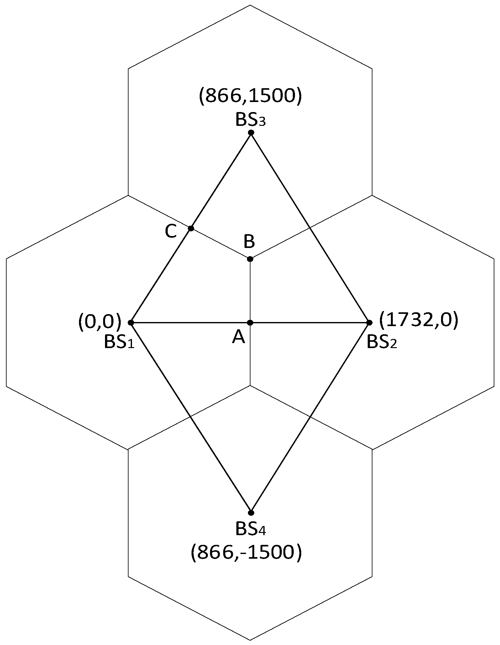
The cell layout shown in Figure 2 is used to test the performance of the proposed location algorithms. Simulations were performed for a micro-cellular environment with cells of radii 1 km and the four BSs in three possible configurations as noted in Section 2. Without a loss of generality, the coordinates of the available BSs expressed in meters are set to BS₁ (0, 0), BS₂ (1732, 0), BS₃ (866, 1500), and BS₄ (866, –1500), respectively.

The MS location expressed in meters is chosen randomly according to a uniform distribution within the area covered by the polygon formed by the points BS₁, A, B, and C, as shown in Figure 2. This means that the MS coordinates have the global constraints given by the region of interest: down_min(1) = BS_1x, down_min(2) = BS_1y, up_max(1) = A_x, and up_max(2) = C_y. These constraints are included in Equation (25). It should be noted that the constraints (21) apply to the whole region of interest of BS₁ABC.

The initial populations (PSO, and PSO-TVAC) are randomly distributed within the search space area limited by (17)–(21). After applying the Chaotic Opposition-based initialization procedure described in Section 3.3, the final form of an initial population for the COPSO-TVAC algorithm is obtained. Then, each corresponding algorithm is further executed as a constrained optimization algorithm.

The procedures use the penalty functions which penalize infeasible solutions by increasing their fitness values in proportion to the degree of violation of the constraints given by (16) for the initial population (t = 0) and populations generated during the iterative process (t > 0). If the penalty is too low, the feasible region may never be reached. On the other hand, if the penalty is too high, the feasible region will be reached so fast, mostly at random, and the probability of getting trapped in the local optimum might be very high [49]. According to [50], the selected penalized form of the fitness function uses the parameters q_i, which define the constraints (16):

$$F_p\left({\mathsf{\theta }}_{\mathit{e}}\right)=\left\{\begin{array}{l}{F}_a\left({\mathsf{\theta }}_{\mathit{e}}\right)+{{\displaystyle \sum }}_{i=1}^4{q}_i,t=0\left(\mathrm{COPSO}-\mathrm{TVAC}\right)\\ F\left({\mathsf{\theta }}_{\mathit{e}}\right)+{{\displaystyle \sum }}_{i=1}^4{q}_i,t=0\left(\mathrm{other}\mathrm{algorithms}\right)\end{array}\right.$$

(57)

$$F_p\left({\mathsf{\theta }}_{\mathit{e}}\right)=F\left({\mathsf{\theta }}_{\mathit{e}}\right)+\left(t/2\right){{\displaystyle \sum }}_{i=1}^4{q}_i,t>0(\mathrm{all}\mathrm{algorithms})$$

(58)

where the parameters q_i are estimated during iterations. The standard deviation of the Gaussian measurement errors is set at 1.5% of the corresponding distance, regardless of the type of environment [17]. Regarding the NLOS effects in the simulation, as a very realistic scenario, the mean of the exponential NLOS error is given by the nonlinear function (11) of the corresponding distance and the factor of the environment (k₂). This factor is obtained based on the parameters of the propagation model given in [10,47].

In this paper, we explore the suburban and urban-type environments, which we will focus on in more detail later. According to the cell geometry shown in Figure 2, one thousand independent measurements with different location geometries were performed in the region of interest. For each averaged measurement (3) associated with a randomly selected location geometry, each algorithm has been independently run 30 times, and the average results between the best fitnesses are obtained.

All simulation parameters of the PSO, the PSO-TVAC, and the COPSO-TVAC algorithms are dimensionless and are presented in

Table 1. The simulation parameters of the PSO, PSO-TVAC, and COPSO-TVAC algorithms.

Simulation Parameter	PSO	PSO-TVAC	COPSO-TVAC
Population size (N)	20	20	20
Dimension of the search space (n)	4–6	4–6	4–6
Sample size (M)	50	50	50
Maximum iteration number (T)	100	100	100
Value of factor k1	0.015	0.015	0.015
Value of factor k2 (suburban)	100.06	100.06	100.06
Value of factor k2 (urban)	133.42	133.42	133.42
Cognitive acceleration coefficient (c1)	2	-	-
Social acceleration coefficient (c2)	2	-	-
Initial value of cognitive coefficient (c1i)	-	2.5	2.5
Final value of cognitive coefficient (c1f)	-	0.5	0.5
Initial value of social coefficient (c2i)	-	0.5	0.5
Final value of social coefficient (c2f)	-	2.5	2.5
Initial value of LDIW/CDIW factor (ωmax)	0.9	0.9	0.9
Final value of LDIW/CDIW factor (ωmin)	0.4	0.4	0.4
Weighting factor kp	0.15	0.15	0.15
Initial value of a logistic map in (44) and (45)	-	-	0.7

.

The pseudocode of the COPSO-TVAC for optimization problem (22) is described by Algorithm 3 as follows:

Algorithm 3 COPSO-TVAC algorithm for optimization problem (22)

1:  Initialization: 2:  Specify the parameters of the COPSO-TVAC algorithm using Table 1; 3:  Generate the initial population through the initialization procedure described in Section 3.3; 4:  Generate the zero initial velocity and set the position limit according to (17)–(21); 5:  Main part of the algorithm: 6:        fort = 1:T do 7:          Update the CDIW parameter using (44); 8:          Update the TVAC coefficients using (35) and (36); 9:          fori = 1:N do 10:            fork = 1:n do 11:                Update the velocity using (43); 12:                if vik (t + 1) < −vkmax, then vik (t + 1) = −vkmax; According to (28) 13:                  else if vik (t + 1) > vkmax, then vik (t + 1) = vkmax; According to (28) 14:                end if 15:                Update the position using (31); 16:                if xik (t + 1) < downk, then xik (t + 1) = downk; According to (25) 17:                  else if xik (t + 1) > upk, then xik (t + 1) = upk; According to (25) 18:                end if 19:            end for 20:          Evaluate the fitness of each particle according to fitness function (13) and constraints given by (16); 21:          Update the individual-best and global-best positions using (33) and (34); 22:          end for 23:      end for 24:      Return the best global solution;

The best algorithm in the session with one thousand measurements must satisfy three categories: the best average location accuracy, the best average convergence properties, and the best efficiency from a statistical point of view. The static positioning model (2) uses a sample of 50 measurements, while the population size for each algorithm is set to 20 particles (see Table 1). After generating the initial population of the COPSO-TVAC algorithm, a fitness evaluation is performed for all particles. In the next steps, all the relevant parameters are updated. The algorithm stops after reaching a maximum number of 100 iterations. Since mobile positioning is a real-time application, this number of iterations is selected to balance the time complexity and accuracy of the proposed algorithms. Finally, the coordinates obtained in the final iteration determine the MS location estimation.

In this section, experiments are conducted to evaluate the localization performance and to perform the analysis of the benefits of the proposed modifications incorporated into the COPSO-TVAC algorithm. In this regard, the presentation of the experimental results is divided into four subsections, described below.

5.1. Localization Performance

To verify the localization performance of the proposed metaheuristic algorithms, we compared them to the classical positioning methods such as gradient-based algorithms (the Levenberg–Marquardt (LM) and the Trust Region Reflective (TRR) algorithm) [7,8], and the Taylor Series-based Least Squares algorithm (TSLS) [13]. The objective function (13) is an excellent benchmark function for comparing the proposed metaheuristics with gradient methods.

Typically, the iterative-optimization-based algorithms can achieve a better location accuracy than noniterative algorithms, especially when there are relatively large NLOS errors in TOA measurements.

As is known, the TOA measurements are converted into a set of circulars in Equation (2), from which the MS location can be determined with the knowledge of the BS geometry.

The gradient-based optimization methods (GB) all rely on the first and second derivatives of the nonlinear function to iteratively find the minimum of (13). However, if the objective function has many local minima, gradient methods will converge to the local optimum that is closest to the initial estimate. An advantage of these methods is that they are computationally efficient [51].

The LM algorithm [7] and the TRR algorithm [8] give very similar results and interpolate between the Gauss–Newton algorithm (GN) and the method of gradient descent. The LM does not require constraints, while the TRR allows only bounds or linear equality constraints, but not both. They are more robust than the GN algorithm, which means that in many cases, they find a solution even if it starts very far from the final minimum [51]. When the number of equations (number of BSs) is less than the number of unknowns, then the TRR algorithm is not applicable. Therefore, in a scenario with three or four NLOS BSs, we used the LM algorithm, while in a scenario with two NLOS BSs, we used the TRR algorithm.

The basic idea of the linear localization methodology is to convert the nonlinear expressions (3) into a set of linear equations, assuming that the NLOS errors are sufficiently small. The Weighting Linear Least Squares (WLLS) algorithm is a weighted version of the LLS scheme, and it provides a higher localization accuracy, although the mean and covariance of the measurement errors in the linear equations are required for the weight computation [11]. Intuitively, the LOS measurements should be weighted more than the NLOS terms.

The results provided by the WLLS algorithm are often used as the initial location estimates for the TSLS algorithm. The TSLS method typically requires an initial position estimate close to the true value, otherwise, the convergence cannot be guaranteed. In this algorithm, a set of nonlinear measurement equations is linearized by expanding them in a Taylor Series at a point, which is an estimate of the true position initially, and keeping only the terms below the second-order [12,13]. The set of linearized equations is solved to produce a new approximate position, and the iterative process continues until the predefined criterion is satisfied.

The TSLS algorithm is the preferred option for position estimation in NLOS situations with small NLOS errors due to its good trade-off between accuracy and complexity [12]. In this paper, results provided by the TSLS algorithm are used as the initial location estimates for the TRR and LM algorithms.

The location accuracy expressed in length units is measured in terms of the Root Mean Square Error (RMSE) between the exact MS location and the estimated MS location.

Generally, the RMS location error is obtained from the average of N_t independent measurements as follows:

$$RMSE=\sqrt{MSE}=\sqrt{\frac{1}{N_t}{{\displaystyle \sum }}_{i=1}^{N_t}[{(x-{\widehat{x}}_i)}^2+{(y-{\widehat{y}}_i)}^2]}$$

(59)

The minimum of (59) is denoted as Root Minimum Mean Square Error (RMMSE) and defined by (56):

$$RMMSE=\sqrt{MMSE}=\sqrt{GCRLB\left(x\right)+GCRLB\left(y\right)}$$

(60)

It can be seen that GCRLB (MMSE) (56), RMMSE (60), and MSE or RMSE (59) are all defined for the static MS location. Hence, it makes sense to compare GCRLB (MMSE) with MSE obtained over sufficiently many trials at that location. For that reason, in our experiment where the MS randomly changes position, we introduce an approximately accurate measure, the so-called Average GCRLB (AGCRLB) or Average MMSE (AMMSE), as the average parameter (56) for all trials (N_t = 1000) in the location area BS¹ABC, as follows:

$$AGCRLB=AMMSE=\frac{1}{N_t}{{\displaystyle \sum }}_{i=1}^{N_t}MMSE\left[\mathsf{\theta }\left(i\right)\right]$$

(61)

Finally, for the accuracy limit expressed in length units, we adopt Root AMMSE (RAMMSE) as:

$$RAMMSE=\sqrt{AMMSE}=\sqrt{\frac{1}{N_t}{{\displaystyle \sum }}_{i=1}^{N_t}\mathrm{tr}\left\{{\mathit{J}}^{-1}\left[\mathsf{\theta }\left(i\right)\right]\right\}}$$

(62)

The accuracy measure (62) is then compared to RMSE, expressed as follows:

$$RMSE=\sqrt{MSE}=\sqrt{\frac{1}{N_t}{{\displaystyle \sum }}_{i=1}^{N_t}[{(x_i-{\widehat{x}}_i)}^2+{(y_i-{\widehat{y}}_i)}^2]}$$

(63)

The above equation differs from (59) in that it refers to the case where the position of the MS is different for each simulation trial.

From the aspect of servicing telecommunication traffic and the number of subscribers, the micro-cellular structure of the cellular network (radii of cells are in the range of 0.2 km to 2 km) is planned mainly in suburban and urban areas. Therefore, in this paper, we describe realistic NLOS situations, which occur in the suburban and the urban environment. It is assumed that the same environmental conditions apply to all BSs due to the small spatial matrix of the positioning, as shown in Figure 2.

These environments are represented by the factor k₂, shown in Table 1. This factor determines the levels of the mean value of the presented NLOS errors (11) as a function of the propagation characteristics of the corresponding environments.

Without strictly going into the mathematical details that can be found in [10,47,52], we rewrite (11) in the following way:

$${\lambda }_i=c{T}_e\mathit{exp}(m_z+\frac{{\sigma }_z^2}{2})d_i^{\epsilon }$$

(64)

where

$$m_z=\frac{\mathit{ln}10}{10}{m}_{\xi }$$

(65)

$${\sigma }_z=\frac{\mathit{ln}10}{10}{\sigma }_{\xi }$$

(66)

c is the speed of light, as earlier, T_e is the median value of the delay spread at distance d = 1 km (which is 0.3 μs for the suburban and 0.4 μs for the urban environment, respectively), ε is an exponent that typically has a value of 0.5, and ξ is a lognormal random variable.

So, it can be written:

$$k_2=c{T}_e\mathit{exp}(m_z+\frac{{\sigma }_z^2}{2})$$

(67)

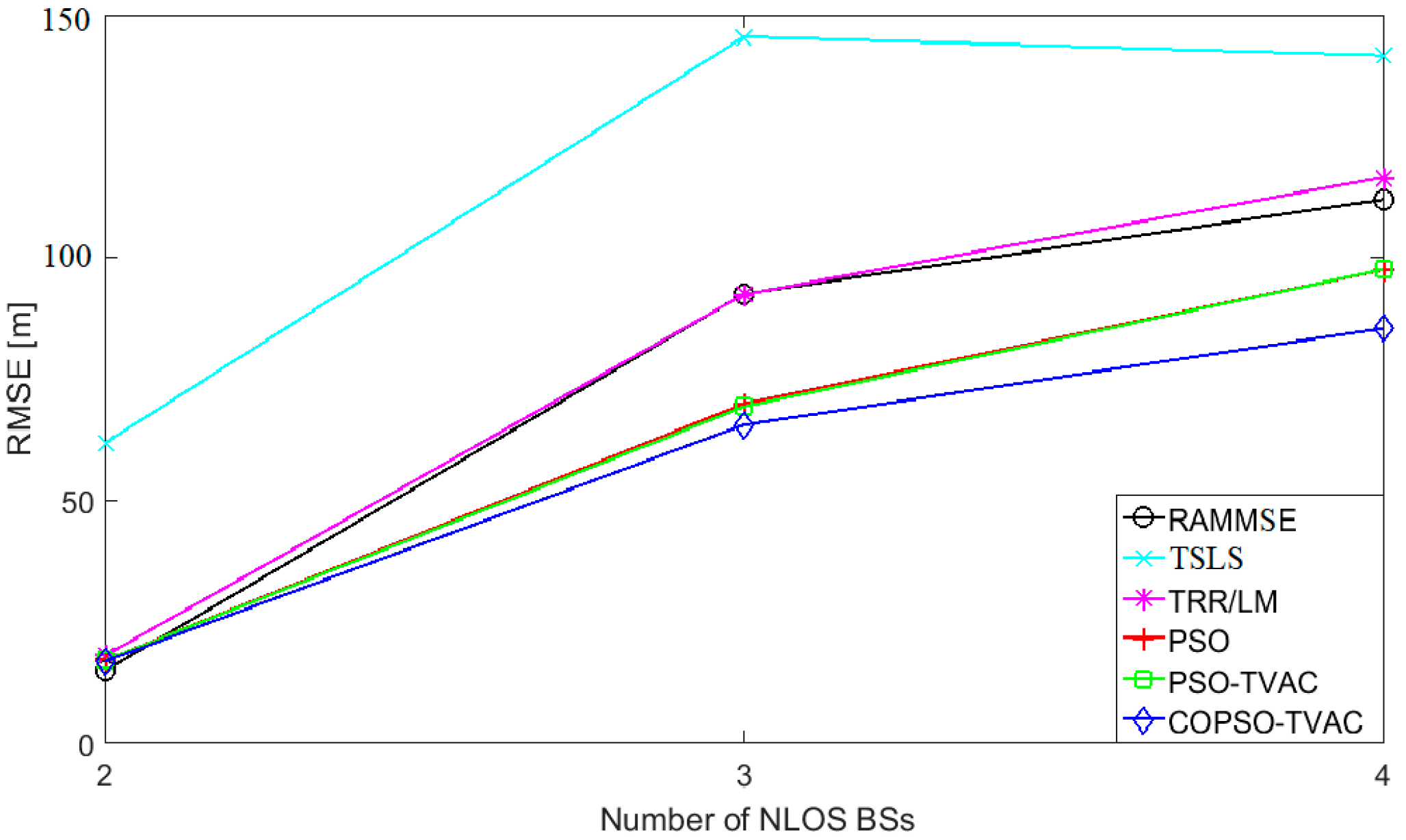
Specifically, 10logξ is a Gaussian random variable with a mean m_ξ and standard deviation σ_ξ. Usually m_ξ = 0 dB, while σ_ξ = 2 dB. When the given values are included in (65)–(67), the values for the factor k₂ shown in Table 1 are obtained. In this case, the urban and suburban environments differ by factor T_e.

Table 2. Location accuracy for the considered algorithm [m], the suburban environment.

Number of NLOS BSs	RAMMSE	RMSE
		TSLS	TRR/LM	PSO	PSO-TVAC	COPSO-TVAC
2	14.93	61.80	18.05	17.08	17.07	16.89
3	92.53	145.44	92.42	69.91	69.30	65.56
4	111.95	141.60	116.51	97.47	97.54	85.43

and

Table 3. Location accuracy for the considered algorithm [m], the urban environment.

Number of NLOS BSs	RAMMSE	RMSE
		TSLS	TRR/LM	PSO	PSO-TVAC	COPSO-TVAC
2	16.92	111.87	18.89	18.26	18.06	17.84
3	122.99	203.31	128.47	87.47	87.17	82.17
4	149.08	193.81	159.02	126.43	126.38	103.45

, as well as Figure 3 and Figure 4, summarize the results of RAMMSE [4] and RMSE expressed in meters for the considered algorithms (the TSLS [13], the LM [7], the TRR [8], the PSO [22], the PSO-TVAC [36], and the COPSO-TVAC), for the suburban and the urban environment in scenarios with the different numbers of NLOS BSs.

As can be seen in Section 4, the GCRLB depends on the location geometry (see Equations (49) and (50)) and the variance of LOS and NLOS errors (see Equations (53)–(55)). The variance of LOS and NLOS errors depends on the true distance between the MS and the BSs, i.e., the location geometry (see Equations (10) and (11)).

Thus, the location accuracy for the positioning scenarios considered in this paper depends primarily on the location geometry. Because the MS locations are randomly selected inside the polygon BS₁ABC, as shown in Figure 2, the average location accuracy (RMSE) in more repeated sessions with one thousand averaged measurements (3) for the positioning scenarios with the same number of the NLOS BSs in the same environment is different.

Such differences in values for the RMSE in the same environment are up to 5 m for the configuration with 2 NLOS BSs, up to 12 m for the configuration with 3 NLOS BSs, and up to 17 m for the configuration with 4 NLOS BSs. The value for RAMMSE hardly changes for the same scenario in the same environment. This paper presents the most favorable values for the RMSE for all three scenarios in both environments.

As can be seen from the attached, the type of environment and the number of NLOS BSs have a great influence on the RMSE. The mean value of the NLOS error is higher in the urban environment (higher value of the factor k₂), so the location error is higher for the same positioning scenario. In some cases, the impact of the environment is stronger than the impact of the number of NLOS BSs. For example, the TSLS and TRR/LM algorithms produce higher values for RMSE in the case of scenarios with three NLOS BSs in the urban environment than in the case of scenarios with four NLOS BSs in the suburban environment, as shown in Table 3 and

Table 4. Average ranks computed through the Friedman test for the proposed metaheuristic algorithms across different NLOS scenarios, at the significance level of 0.05.

Algorithm	Scenario						Mean Ranking	Rank
	2 NLOS BSs Suburban	2 NLOS BSs Urban	3 NLOS BSs Suburban	3 NLOS BSs Urban	4 NLOS BSs Suburban	4 NLOS BSs Urban
PSO	2.68	2.68	2.74	2.78	2.49	2.52	2.64	3
PSO-TVAC	1.83	1.77	1.76	1.76	1.75	1.81	1.78	2
COPSO-TVAC	1.48	1.53	1.49	1.45	1.74	1.65	1.55	1
Friedman p value	0.000	0.000	0.000	0.000	0.000	0.000

. However, the largest jump in the effective error (in both environments) occurs when the number of NLOS BSs exceeds the number of LOS BSs (the scenario with three NLOS BSs).

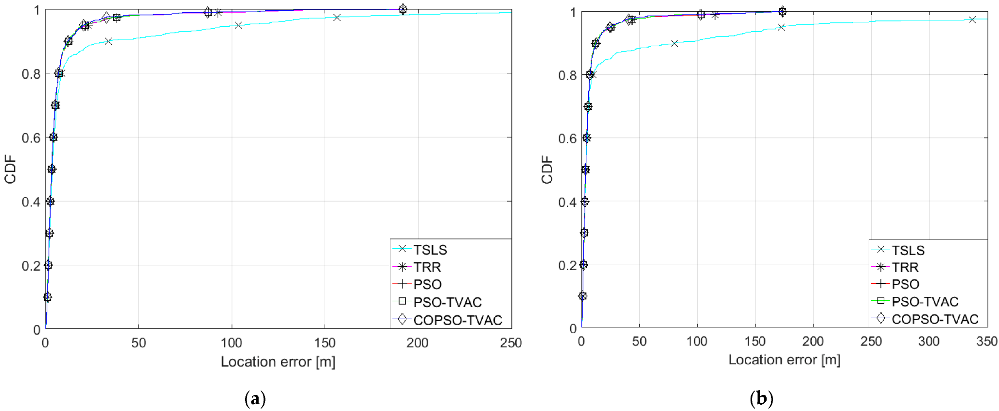
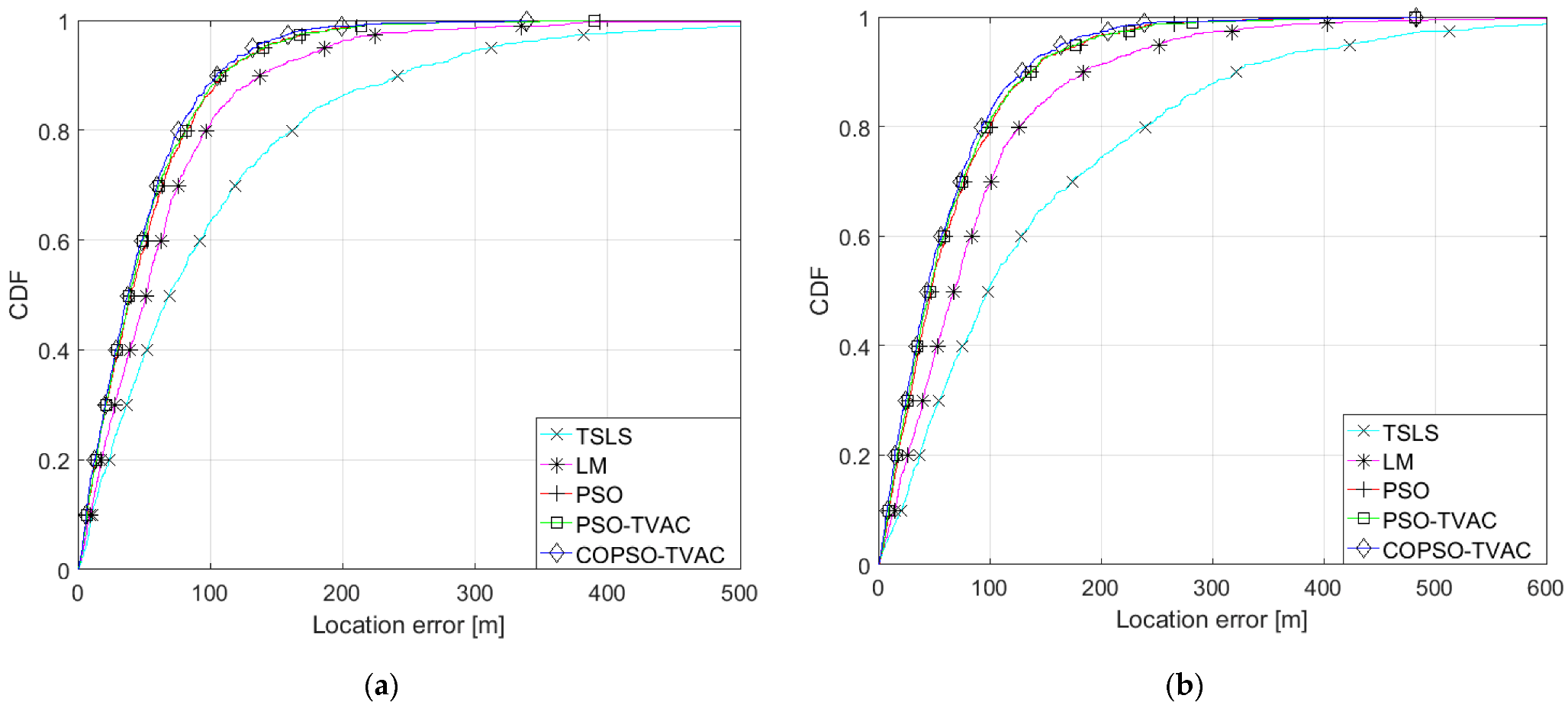
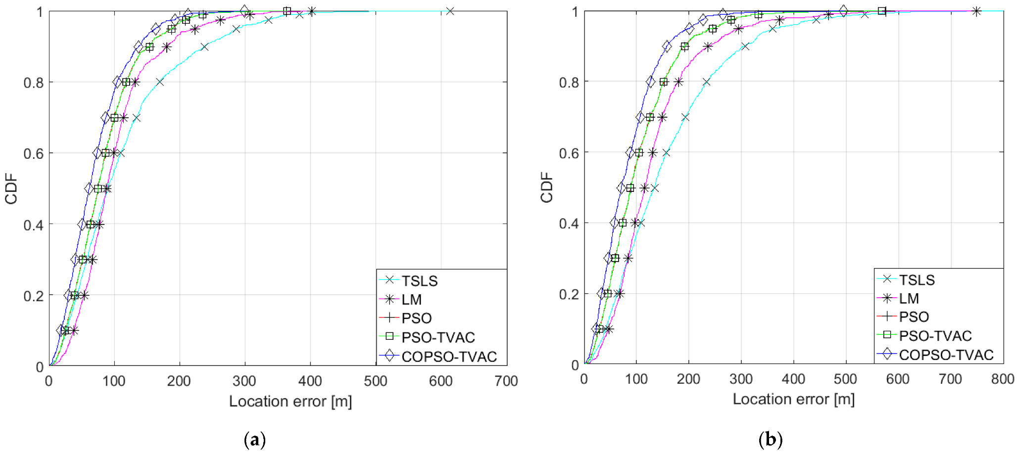
The location accuracy using the proposed algorithms can also be represented by the Cumulative Distribution Function (CDF) curves of location errors.

The CDFs curves of location errors depending on the propagation environment for the scenarios with two, three, and four NLOS BSs are shown in Figure 5, Figure 6 and Figure 7.

Compared with the existing methods (the TSLS [13], the LM [7], and the TRR [8]), the accuracy of the MS location indeed improved with the proposed metaheuristic algorithms. In all NLOS conditions, the PSO algorithm [22] and the PSO-TVAC algorithm [36] produce very similar and very good results, with the COPSO-TVAC algorithm being better than both. In the case when two NLOS BSs participate, all algorithms except the TSLS algorithm give expected results, which are more or less similar and very close to the RAMMSE. The power of the COPSO-TVAC algorithm is shown in the simulations with three and four NLOS BSs, where it greatly surpasses all other algorithms regardless of the type of environment.

It is interesting to note that metaheuristic algorithms give better results than RAMMSE for the scenarios with three and four NLOS BSs, as shown in Table 2 and Table 3. Namely, as the number of NLOS BSs increases, the nonlinearity of the objective function (13) greatly increases. In this way, the ML estimator becomes more biased, which is the possible reason for obtaining such results [53]. A similar case where the MSE takes lower values than the CRLB can be found in Reference [54]. This fact does not diminish the statistical weight of the RAMMSE metric and does not mask the quality of the obtained results.

5.2. Convergence Properties

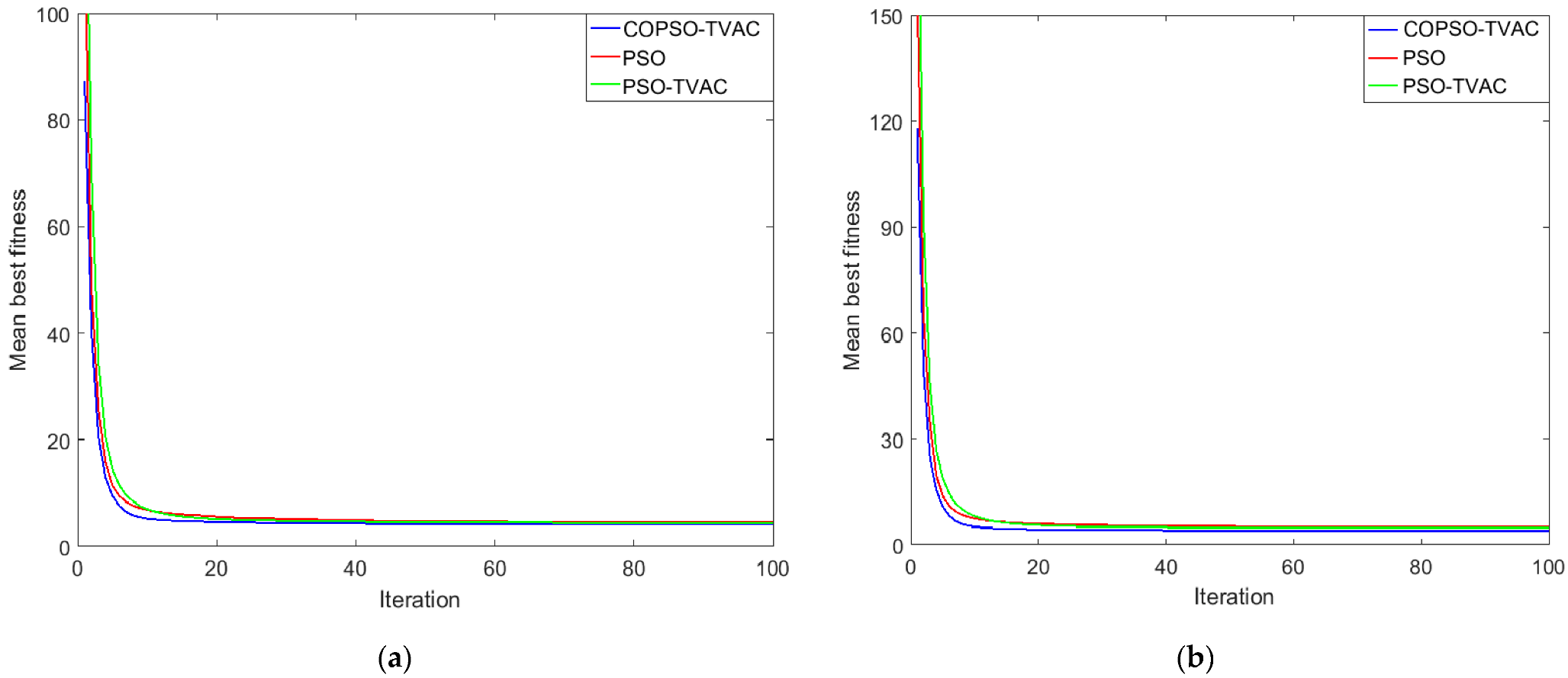
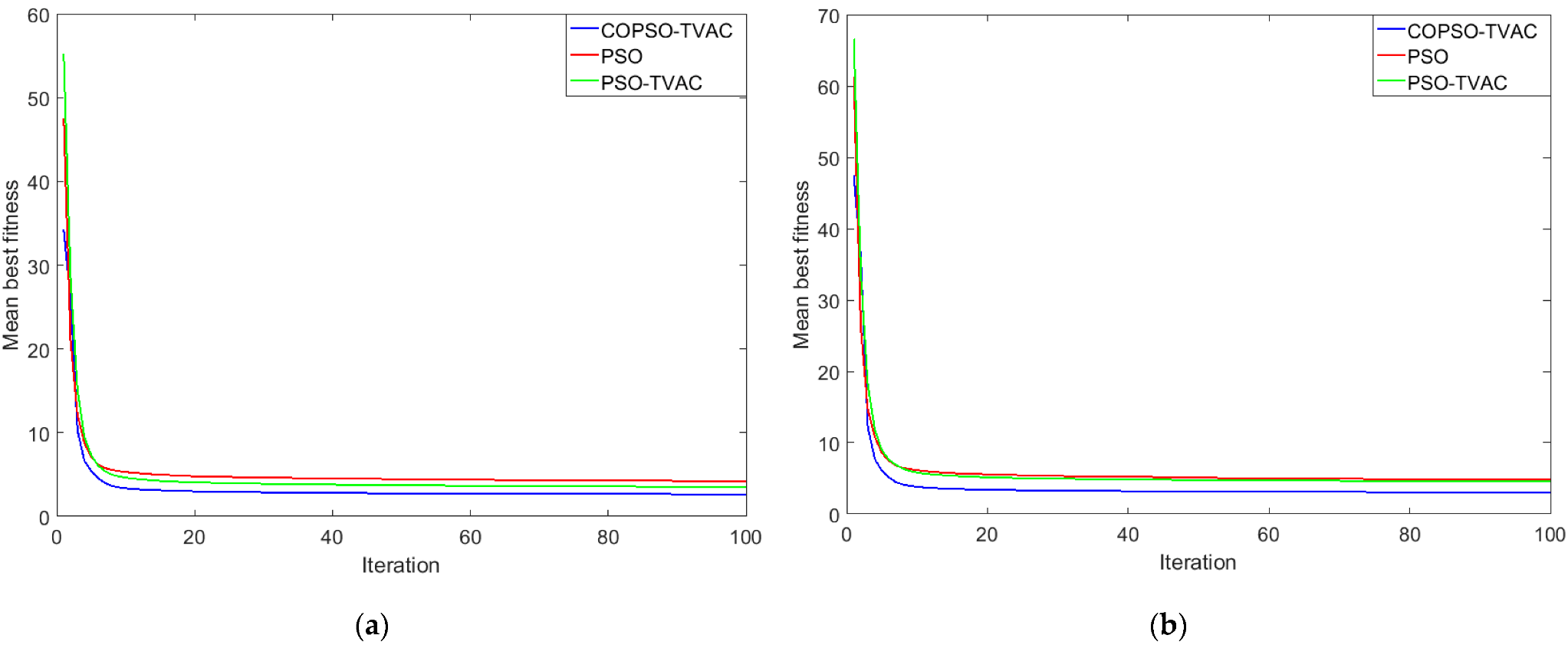
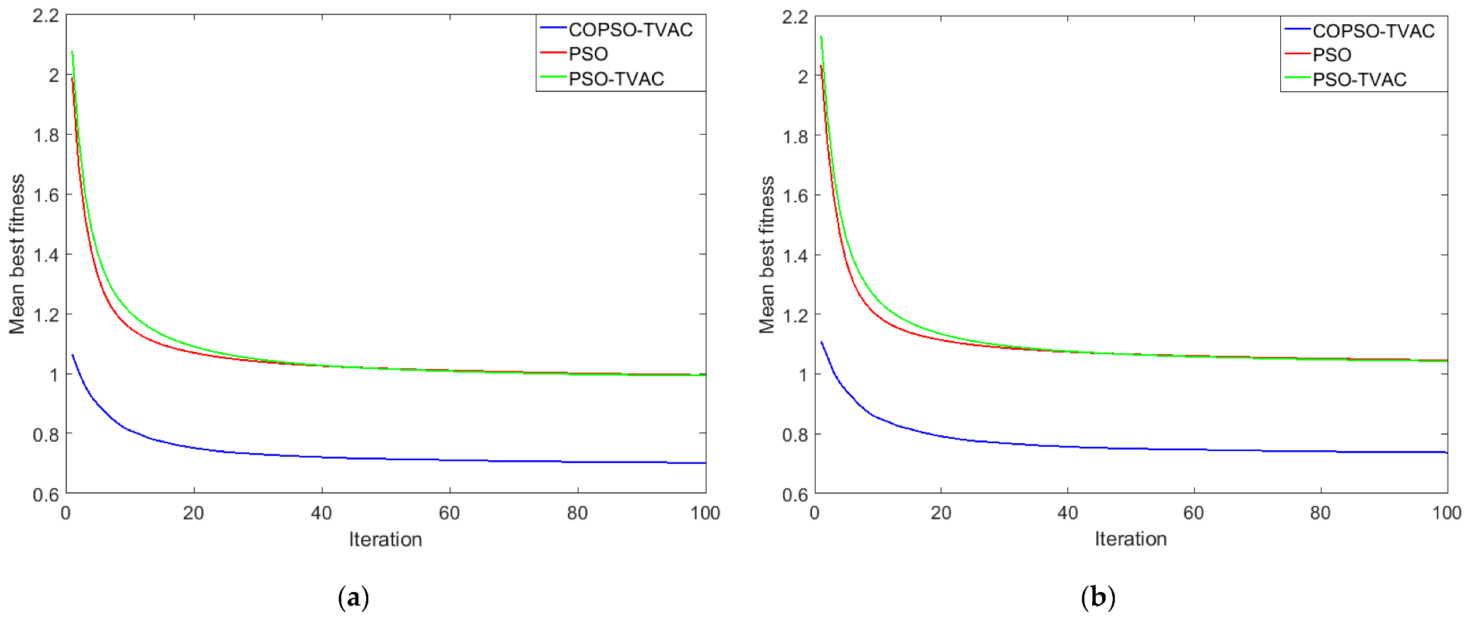
The convergence characteristics show the change in the average fitness function during algorithm execution. It makes sense to compare these characteristics from the first iteration (for the same ML fitness function (13)). The convergence properties of the given metaheuristic algorithms across environments for all scenarios are shown in Figure 8, Figure 9 and Figure 10.

Note that the mean of the best fitness is dimensionless, and that the penalty functions are included in it.

It can be concluded that the COPSO-TVAC algorithm has better convergence characteristics than the PSO and the PSO-TVAC algorithms in the presented referent situations. Due to a good initialization and searching procedure based on chaos, the COPSO-TVAC algorithm more successfully avoids traps at the local optimum than the other algorithms, as shown in Figure 8, Figure 9 and Figure 10. The convergence rate of all three algorithms does not significantly degrade with a more unfavorable environment or an increase in the number of NLOS BSs.

5.3. Statistical Comparison of the Proposed Metaheuristic Algorithms

In this subsection, a simulation study has been performed to demonstrate the effectiveness of the proposed COPSO-TVAC algorithm. From the statistical point of view, to evaluate the performance of the proposed metaheuristic algorithms, the mean value of the best fitnesses after 30 runs has been employed as the metric of the quality of the obtained solution for each averaged measurement (3). Then, such metrics of the proposed algorithms for all measurements are analyzed and compared using some non-parametric statistical test. As there are more than two algorithms for comparison, the overall performance of the considered algorithms has been compared using the Friedman test [55]. The Friedman non-parametric test can be used to determine the significant differences in performance between two or more algorithms. In this statistical test, the algorithm with a minimum rank value is considered the algorithm with the best performance.

In this regard, Table 4 shows the average ranks obtained according to the Friedman test for the considered algorithms in different simulation scenarios. This statistical test has been applied with a significance level of α = 0.05. From Table 4, it can be noted that the p values computed through the Friedman test for different simulation scenarios are minor and less than 0.05. Therefore, this means that there is a significant difference in performance between the considered metaheuristic algorithms. Furthermore, it can be observed that the proposed COPSO-TVAC algorithm outperforms other algorithms for all experimental situations, which demonstrates the effectiveness of the modifications proposed in this paper.

5.4. Computational Complexity of the Considered Algorithms

If the computational complexity of the iterative algorithms is expressed per iteration, then the complexity of the TSLS algorithm is O($n_c^2{N}_b$), where n_c is the number of the target MS coordinates, and N_b is the number of BSs [11]. It is a low-complexity and low-accuracy iterative algorithm. The complexity of the gradient-based algorithms is O(n³) [51]. The computational complexity of the PSO and the PSO-TVAC algorithms is O(nN) [31]. The computational costs of these metaheuristic algorithms are dramatically reduced by using a minimum population size of 20 particles.

The implementation of chaos into metaheuristic algorithms does not significantly increase the complexity of the original algorithms. However, in opposition-based algorithms, the opposition population is used in parallel with the original population, so the size of the effective population is twice as large. The complexity of such algorithms increases in this ratio and amounts to O(2nN) [42]. Fortunately, the opposition population is only used to generate the initial population. Thus, the computational complexity of the COPSO-TVAC algorithm is approximately equal to the complexity of the original algorithms and is O(nN).

The average computation time in searching for the global optimum has been determined on the same PC with a 2.2 GHz CPU and 4 GB of RAM. The MATLAB R2016b software package (MathWorks, Natick, MA, USA) was used. In this way, based on the considered simulation scenarios, a comparison between the average computation times of the considered algorithms expressed in milliseconds is shown in

Table 5. Average computation times of the considered algorithms by different NLOS configurations, expressed in [ms].

Algorithm	Configuration
	2 NLOS BSs	3 NLOS BSs	4 NLOS BSs
TSLS	3.03	3.16	3.20
TRR	29.50	-	-
LM	-	32.68	34.94
PSO	11.15	12.99	13.42
PSO-TVAC	11.39	13.58	14.24
COPSO-TVAC	12.04	13.88	14.88

.

The proposed metaheuristic methods provide an excellent location accuracy with a moderate computational complexity. Table 5 shows that the TSLS algorithm has the fastest implementation among the considered algorithms, while there is no significant difference between the proposed metaheuristic algorithms. Based on the results of the analysis of the location accuracy in Table 2 and Table 3, the results in Table 5 indicate that the proposed COPSO-TVAC algorithm achieves the best compromise between the location accuracy and the average computation time in searching for the global optimum.

6. Conclusions and Future Scope

The NLOS propagation is one of the main problems that affect positioning performance. In this paper, we investigated the methods for mitigating the NLOS errors that corrupt the TOA range measurements in the micro-cellular radio environment.

To reduce the exponential NLOS errors, the proposed methods utilize all the feasible intersections which are generated by four TOA circles to estimate the MS location.

To solve the nonlinear and nonconvex ML location problem (22) even under highly NLOS conditions, an improved version of the PSO-TVAC algorithm, based on the hybridization of the Opposition-Based Learning, Chaos Search, and TVAC strategies, has been proposed. The simulation results show that the proposed COPSO-TVAC algorithm provided a superior localization performance under different NLOS conditions compared to the original PSO and PSO-TVAC algorithms as well as the traditional location algorithms such as the Least Squares and Gradient-based algorithms.

The results of the statistical and experimental analysis confirm that the COPSO-TVAC algorithm outperforms the compared metaheuristic algorithms in terms of the best solutions and convergence behavior. Considering the above facts, the modifications proposed in this algorithm can improve the overall optimization performance.

Future work can be focused on the application of the Crow Search Algorithm (CSA) to the problems of cellular positioning in NLOS conditions.

References

1. Silventoinen, M.I.; Rantalainen, T. Mobile station emergency locating in GSM. In Proceedings of the 1996 IEEE International Conference on Personal Wireless Communications, New Delhi, India, 21–21 February 1996; pp. 232–238. [Google Scholar]
2. Chan, Y.T.; Tsui, W.Y.; So, H.C.; Ching, P.C. Time-of-arrival based localization under NLOS conditions. IEEE Trans. Veh. Technol. 2006, 55, 17–24. [Google Scholar] [CrossRef]
3. Cong, L.; Zhuang, W. Non-line-of-sight error mitigation in TDOA mobile location. In Proceedings of the GLOBECOM’01, IEEE Global Telecommunications Conference (Cat. No.01CH37270), San Antonio, TX, USA, 25–29 November 2001; pp. 680–684. [Google Scholar]
4. Qi, Y. Wireless Geolocation in a Non-Line-of-Sight Environment. Ph.D. Thesis, Princeton University, Princeton, NJ, USA, November 2003. [Google Scholar]
5. Mensing, C.; Plass, S. Positioning algorithms for cellular networks using TDOA. In Proceedings of the 2006 IEEE International Conference on Acoustics, Speech and Signal Processing, Toulouse, France, 14–19 May 2006; pp. 513–516. [Google Scholar]
6. Ouyang, R.W.; Wong, A.K. An Enhanced ToA-based Wireless Location Estimation Algorithm for Dense NLOS Environments. In Proceedings of the 2009 IEEE Wireless Communications and Networking Conference, Budapest, Hungary, 5–8 April 2009; pp. 1–6. [Google Scholar]
7. Wang, Y.; Wu, Q.; Zhou, M.; Yang, X.; Nie, W.; Xie, L. Single base station positioning based on multipath parameter clustering in NLOS environments. EURASIP J. Adv. Signal Process. 2021, 2021, 20. [Google Scholar] [CrossRef]
8. Ruble, M.; Guvenc, I. Wireless localization for mmWave networks in urban environments. EURASIP J. Adv. Signal Process. 2018, 2018, 35. [Google Scholar] [CrossRef] [PubMed]
9. Riba, J.; Urruela, A. A non-line-of-sight mitigation technique based on ML-detection. In Proceedings of the 2004 IEEE International Conference on Acoustics, Speech and Signal Processing, Montreal, QC, Canada, 17–21 May 2004; pp. 151–153. [Google Scholar]
10. Chen, P.C. A non-line-of-sight error mitigation algorithm in location estimation. In Proceedings of the WCNC, 1999 IEEE Wireless Communications and Networking Conference (Cat. No.99TH8466), New Orleans, LA, USA, 21–24 September 1999; pp. 316–320. [Google Scholar]
11. Cheung, K.W.; So, H.C.; Ma, W.K.; Chan, Y.T. Least squares algorithms for time-of-arrival-based mobile location. IEEE Trans. Signal Process. 2004, 52, 1121–1130. [Google Scholar] [CrossRef] [Green Version]
12. Yu, K.; Guo, Y.J. NLOS Error Mitigation for Mobile Location Estimation in Wireless Networks. In Proceedings of the 2007 IEEE 65th Vehicular Technology Conference—VTC2007-Spring, Dublin, Ireland, 22–25 April 2007; pp. 1071–1075. [Google Scholar]
13. Kocur, D.; Švecova, M.; Kažimir, P. Determining the Position of the Moving Persons in 3D Space by UWB Sensors using Taylor Series Based Localization Method. Acta Polytech. Hung. 2019, 16, 45–63. [Google Scholar] [CrossRef]
14. Wang, X.; Wang, Z.; O’Dea, B. A TOA-based location algorithm reducing the errors due to non-line-of-sight (NLOS) propagation. IEEE Trans. Veh. Technol. 2003, 52, 112–116. [Google Scholar] [CrossRef]
15. Venkatesh, S.; Buehrer, R.M. NLOS mitigation using linear programming in UWB location-aware networks. IEEE Trans. Veh. Technol. 2007, 56, 3182–3198. [Google Scholar] [CrossRef]
16. Venkatesh, S.; Buehrer, R.M. A linear programming approach to NLOS mitigation in sensor networks. In Proceedings of the 2006 5th International Conference on Information Processing in Sensor Networks, Nashville, TN, USA, 19–21 April 2006; pp. 301–308. [Google Scholar]
17. Yu, K.; Guo, Y.J. Improved Positioning Algorithms for Nonline-of-Sight Environments. IEEE Trans. Veh. Technol. 2008, 57, 2342–2353. [Google Scholar]
18. Yang, X.S. Engineering Optimization: An Introduction with Metaheuristic Application, 1st ed.; John Wiley & Sons, Inc.: Hoboken, NJ, USA, 2010; pp. 1–28. [Google Scholar]
19. Yang, X.S. Nature-Inspired Optimization Algorithms, 1st ed.; Elsevier, Inc.: London, UK, 2014; pp. 1–42. [Google Scholar]
20. Campos, R.S.; Lovisolo, L. Genetic algorithm optimized DCM positioning. In Proceedings of the 2013 10th Workshop on Positioning, Navigation and Communication (WPNC), Dresden, Germany, 20–21 March 2013; pp. 1–5. [Google Scholar]
21. Chen, C.S.; Lin, J.M.; Lee, C.T.; Lu, C.D. The Hybrid Taguchi-Genetic Algorithm for Mobile Location. Int. J. Distrib. Sens. Netw. 2014, 10, 489563. [Google Scholar] [CrossRef] [Green Version]
22. Chen, C.S. A non-line-of-sight error mitigation method for location estimation. Int. J. Distrib. Sens. Netw. 2017, 13, 1–9. [Google Scholar] [CrossRef] [Green Version]
23. Enqing, D.; Yanze, C.; Xiaojun, L. A novel three-dimensional localization algorithm for Wireless Sensor Networks based on Particle Swarm Optimization. In Proceedings of the 2011 18th International Conference on Telecommunications, Ayia Napa, Cyprus, 8–11 May 2011; pp. 55–60. [Google Scholar]
24. Lukic, S.; Simic, M. NLOS Error Mitigation in Cellular Positioning using PSO Optimization Algorithm. Int. J. Electr. Eng. Comput. IJEEC 2018, 2, 48–56. [Google Scholar]
25. Chen, C.S.; Huang, J.F.; Huang, N.C.; Chen, K.S. MS Location Estimation Based on the Artificial Bee Colony Algorithm. Sensors 2020, 20, 5597. [Google Scholar] [CrossRef]
26. Yiang, J.; Liu, M.; Chen, T.; Gao, L. TDOA Passive Location Based on Cuckoo Search Algorithm. J. Shanghai Jiaotong Univ. (Sci.) 2018, 23, 368–375. [Google Scholar]
27. Cheng, J.; Xia, L. An Effective Cuckoo Search Algorithm for Node Localization in Wireless Sensor Network. Sensors 2016, 16, 1390. [Google Scholar] [CrossRef] [Green Version]
28. Tuba, E.; Tuba, M.; Beko, M. Two Stage Wireless Sensor Node Localization Using Firefly Algorithm. In Smart Trends in Systems, Security and Sustainability; Yang, X.S., Nagar, A.K., Joshi, A., Eds.; Springer: Singapore, 2018; Volume 18, pp. 113–120. [Google Scholar]
29. Shi, Y.; Eberhart, R.C. Particle swarm optimization: Developments, applications and resources. In Proceedings of the 2001 Congress on Evolutionary Computation (IEEE Cat. No.01TH8546), Seoul, Korea, 27–30 May 2001; pp. 81–86. [Google Scholar]
30. Shi, Y.; Eberhart, R.C. A modified particle swarm optimizer. In Proceedings of the 1998 IEEE International Conference on Evolutionary Computation, IEEE World Congress on Computational Intelligence (Cat. No.98TH8360), Anchorage, AK, USA, 4–9 May 1998; pp. 69–73. [Google Scholar]
31. Zhang, X.; Zou, D.; Shen, X. A Novel Simple Particle Swarm Optimization Algorithm for Global Optimization. Mathematics 2018, 6, 287. [Google Scholar] [CrossRef] [Green Version]
32. Liang, J.J.; Qin, A.K.; Suganthan, P.N.; Baskar, S. Comprehensive Learning Particle Swarm Optimizer for Global Optimization of Multimodal Functions. IEEE Trans. Evol. Comput. 2006, 10, 281–295. [Google Scholar] [CrossRef]
33. Tanweer, M.R.; Suresh, S.; Sundararajan, N. Dynamic mentoring and self-regulation based particle swarm optimization algorithm for solving complex real-world optimization problems. Inf. Sci. 2016, 326, 1–24. [Google Scholar] [CrossRef]
34. Ratnaweera, A.; Halgamuge, S.K.; Watson, H.A. Self-Organizing Hierarchical Particle Swarm Optimizer with Time-Varying Acceleration Coefficients. IEEE Trans. Evol. Comput. 2004, 8, 240–255. [Google Scholar] [CrossRef]
35. Chaturvedi, K.T.; Pandit, M.; Srivastava, L. Particle swarm optimization with time-varying acceleration coefficients for non-convex economic power dispatch. Int. J. Electr. Power Energy Syst. 2009, 31, 249–257. [Google Scholar] [CrossRef]
36. Fang, J.; Feng, J. Using PSO-TVAC to improve the performance of DV-Hop. Int. J. Wirel. Mob. Comput. 2018, 14, 358–361. [Google Scholar] [CrossRef]
37. Zhang, H.; Shen, J.H.; Zhang, T.N.; Li, Y. An improved chaotic particle swarm optimization and its application in investment. In Proceedings of the 2008 International Symposium on Computational Intelligence and Design, Wuhan, China, 17–18 October 2008; pp. 124–128. [Google Scholar]
38. Tian, D. Particle Swarm Optimization with Chaos-based Initialization for Numerical Optimization. Intell. Autom. Soft Comput. 2018, 24, 331–342. [Google Scholar] [CrossRef]
39. Feng, Y.; Teng, G.F.; Wang, A.X.; Yao, Y.M. Chaotic Inertia Weight in Particle Swarm Optimization. In Proceedings of the Second International Conference on Innovative Computing, Information and Control (ICICIC 2007), Kumamoto, Japan, 5–7 September 2007; p. 475. [Google Scholar]
40. Arasomwan, A.M.; Adewumi, A.O. An Investigation into the Performance of Particle Swarm Optimization Algorithm with Various Chaotic Maps. Math. Probl. Eng. 2014, 2014, 178959. [Google Scholar] [CrossRef]
41. Wang, H.; Li, H.; Liu, Y.; Li, C.; Zeng, S. Opposition-based particle swarm algorithm with cauchy mutation. In Proceedings of the 2007 IEEE Congress on Evolutionary Computation, Singapore, 25–28 September 2007; pp. 4750–4756. [Google Scholar]
42. Mahdavi, S.; Rahnamayan, S.; Deb, K. Opposition-based learning: A literature review. Swarm Evol. Comput. 2018, 39, 1–23. [Google Scholar] [CrossRef]
43. Dong, N.; Wu, C.H.; Ip, W.H.; Chen, Z.Q.; Chan, C.Y.; Yung, K.L. An opposition-based chaotic GA/PSO hybrid algorithm and its application in circle detection. Comput. Math. Appl. 2012, 64, 1886–1902. [Google Scholar] [CrossRef] [Green Version]
44. Gao, W.; Liu, S.; Huang, L. Particle swarm optimization with chaotic opposition-based population and stochastic search technique. Commun. Nonlinear Sci. Numer. Simul. 2012, 17, 25185–25199. [Google Scholar] [CrossRef]
45. Venkatraman, S.; Caffery, J.; You, H.R. A novel ToA location algorithm using LOS range estimation for NLOS environments. IEEE Trans. Veh. Technol. 2004, 53, 1515–1524. [Google Scholar] [CrossRef]
46. Del Peral-Rosado, J.A.; Lopes-Salcedo, J.A.; Zanier, F.; Seco-Granados, G. Position Accuracy of Joint Time-Delay and Channel Estimators in LTE Networks. IEEE Access 2018, 6, 25185–25199. [Google Scholar] [CrossRef]
47. Greenstein, L.J.; Erceg, V.; Yeh, Y.S.; Clark, M.V. A new path-gain/delay-spread propagation model for digital cellular channels. IEEE Trans. Veh. Technol. 1997, 46, 477–485. [Google Scholar] [CrossRef]
48. Guvenc, I.; Cong, C.C. A Survey on TOA Based Wireless Localization and NLOS Mitigation Techniques. IEEE Commun. Surv. Tutor. 2009, 11, 107–124. [Google Scholar] [CrossRef]
49. Mezura-Montes, E.; Flores-Mendoza, J.I. Improved Particle Swarm Optimization in Constrained Numerical Search Space. In Nature Inspired Algorithms for Optimization. Studies in Computational Intelligence, 1st ed.; Chiong, R., Ed.; Springer: Berlin/Heidelberg, Germany, 2009; Volume 193, pp. 299–332. [Google Scholar]
50. Joines, J.A.; Houck, C.R. On the Use of Non-Stationary Penalty Function to Solve Nonlinear Constrained Optimization Problems with GA’s. In Proceedings of the First IEEE Conference on Evolutionary Computation, IEEE World Congress on Computational Intelligence, Orlando, FL, USA, 26–29 June 1994; pp. 579–584. [Google Scholar]
51. Optimization and Data Fitting—DTU Informatics. Available online: http://www2.imm.dtu.dk/pubdb/edoc/imm5938.pdf (accessed on 28 September 2021).
52. Jativa, E.R.; Sanchez, D.; Vidal, J. NLOS Mitigation Based on TOA for Mobile Subscriber Positioning System by Weighting Measures and Geometrical Restrictions. In Proceedings of the 2015 Asia-Pacific Conference on Computer Aided System Engineering, Quito, Ecuador, 14–16 July 2015; pp. 325–330. [Google Scholar]
53. Kay, S.; Eldar, Y.C. Rethinking biased estimation [Lecture Note]. IEEE Signal Process. Mag. 2008, 25, 133–136. [Google Scholar] [CrossRef]
54. Cakir, O.; Kaya, I.; Yazgan, A.; Cakir, O.; Tugcu, E. Emitter Location Finding using Particle Swarm Optimization. Radioengineering 2014, 23, 252–258. [Google Scholar]
55. Derrac, J.; Garcia, S.; Molina, D.; Herrera, F. A practical tutorial on the use of nonparametrical statistical test as a methodology for comparing evolutionary and swarm intelligence algorithms. Swarm Evol. Comput. 2011, 1, 3–18. [Google Scholar] [CrossRef]
Figure 1. Location geometry with the four TOA circles [24].
Electronics 11 02300 g001
Figure 2. The considered cellular system with the four BSs [24].
Electronics 11 02300 g002
Figure 3. RMSE [m] in the function of the number of the NLOS BSs: the suburban environment.
Electronics 11 02300 g003
Figure 4. RMSE [m] in the function of the number of the NLOS BSs: the urban environment.
Electronics 11 02300 g004
Figure 5. CDF of the location error in the scenario with 2 NLOS BSs: (a) the suburban environment; (b) the urban environment.
Electronics 11 02300 g005
Figure 6. CDF of the location error in the scenario with 3 NLOS BSs: (a) the suburban environment; (b) the urban environment.
Electronics 11 02300 g006
Figure 7. CDF of the location error in the scenario with 4 NLOS BSs: (a) the suburban environment; (b) the urban environment.
Electronics 11 02300 g007
Figure 8. The convergence properties of the proposed metaheuristic algorithms in the scenario with 2 NLOS BSs: (a) the suburban environment; (b) the urban environment.
Electronics 11 02300 g008
Figure 9. The convergence properties of the proposed metaheuristic algorithms in the scenario with 3 NLOS BSs: (a) the suburban environment; (b) the urban environment.
Electronics 11 02300 g009
Figure 10. The convergence properties of the proposed metaheuristic algorithms in the scenario with 4 NLOS BSs: (a) the suburban environment; (b) the urban environment.
Electronics 11 02300 g010