ViV-Ano: Anomaly Detection and Localization Combining Vision Transformer and Variational Autoencoder in the Manufacturing Process

Abstract

The goal of image anomaly detection is to determine whether there is an abnormality in an image. Image anomaly detection is currently used in various fields such as medicine, intelligent information, military fields, and manufacturing. The encoder–decoder structure, which learns a normal-looking periodic normal pattern and shows good performance in judging anomaly scores through reconstruction errors showing the differences between the reconstructed images and the input image, is widely used in the field of anomaly detection. The existing image anomaly detection method extracts normal information through local features of the image, but the vision transformer base and the probability distribution are generated by learning the global relationship between image anomaly detection and an image patch that can locate anomalies to extract normal information. We propose Vision Transformer and VAE for Anomaly Detection (ViV-Ano), an anomaly detection model that combines a model variational autoencoder (VAE) with Vision Transformer (ViT). The proposed ViV-Ano model showed similar or better performance when compared to the existing model on a benchmark dataset. In addition, an MVTec anomaly detection dataset (MVTecAD), a dataset for industrial anomaly detection, showed similar or improved performance when compared to the existing model.

1. Introduction

As the smart factory develops, the discovery of abnormal data among the data in manufacturing industry research has become an important and popular research field, and many related studies have been conducted [1,2]. The complexity and the dynamics of manufacturing processes create a variety of anomalies, and the accurate detection and capture of anomalous data is critical for the safe operation of manufacturing processes. For example, in the casting industry, a product that has undergone a manufacturing process with a temperature difference may be produced with unusable quality or may cause an accident such as an explosion during the casting process. Therefore, various studies on aspects such as equipment pressure, bearing vibration, and energy consumption in the production process are conducted at the initial stage of the process. Using these studies and the data generated during production, anomalies can be detected during production before serious problems occur in the process.

However, since it is difficult to clearly define normal and abnormal conditions in anomaly detection, it is difficult to find anomalies when the abnormal pattern is similar to the normal pattern. Many studies have been conducted to detect anomalies, but traditional studies [3,4] have shown normal operation for open datasets. However, when applied to actual data, such methods have a severe class imbalance, so they are difficult to apply without a data label for performance use [5]. Convolutional neural networks (CNNs), algorithms that mimic the structure of a nerve, have shown useful performance in using patterns in image recognition. CNNs receive the data in matrix form to preserve the shape of the image through a convolution layer that extracts the feature and a pooling layer that samples the extracted feature to prevent data loss while converting to the one-dimensional data of the existing feedforward neural network (FNN) [6]. However, the CNN cannot extract the feature by looking at the whole if the architecture depth is not sufficient. Moreover, weight-sharing reduces the operation cost, but the computational cost is too large to perform the convolution operation [7]. In other words, CNNs have a disadvantage in image learning because the model learns only local information and not the global context. However, ViT can learn more image features than CNNs, which only learn local information, because attention operation and patch images are used to additionally learn global contexts.

Research on deep learning in image anomaly detection methods has been steadily progressing. The encoder–decoder method and the method based on generation are often used for image anomaly detection and anomaly localization using deep learning. The encoder–decoder method trains the model while compressing the original image and reconstructing the compressed image to resemble the original image. Anomaly detection is mainly achieved through the differences in this restoration, and in the case of generation-based methods, the distribution of the generated normal data is learned through a distribution that generates an image with a shape similar to that of the original image. Recently, Vision Transformer (ViT) has shown a powerful ability to classify and judge images in computer vision. ViT’s self-attention layer consists of several heads and calculates the self-attention distance, which is the distance between the position of the query patch and the position referenced by the patch, for each head [8]. The head of ViT is a mixture of local and global information even in the lowest layer, so the information is smoothly transferred from the lower layer to the higher layer. Since there is no bias in ViT, there is a significant need for pre-learning data. If the dataset is small, bias is not present in ViT, so comparing pros and cons, CNN is still preferred. The preferred structure for each situation is also under study [9]. Variational autoencoders (VAEs) are generative models that can increase the performance of models in learning stochastic factors [10]. In addition, a VAE is a reconstruction-based model, so better results can be obtained for anomaly detection.

In this paper, we propose a model for detecting anomalies during the manufacturing process:

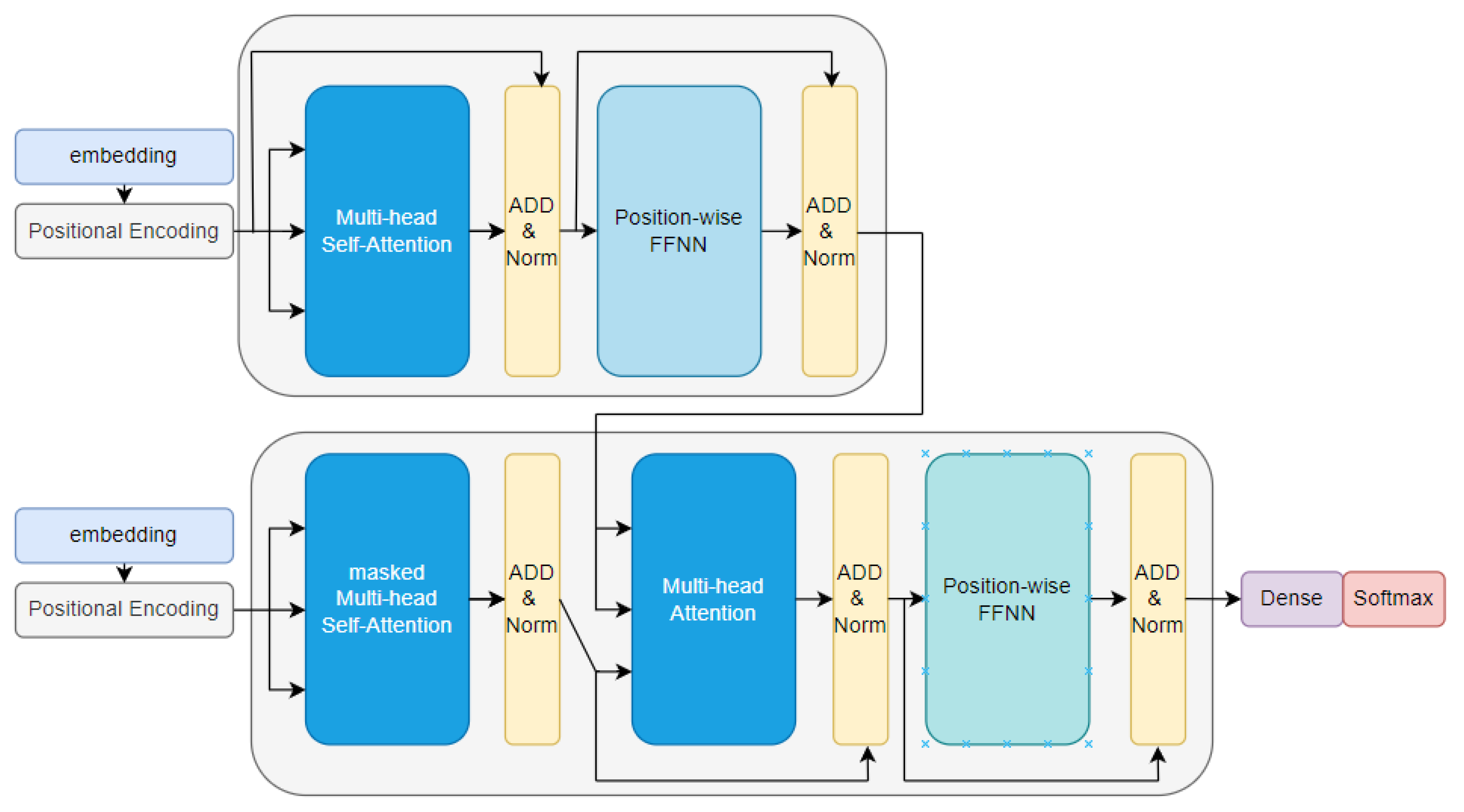
• The image applies the ViT method in the area to be analyzed. ViT has word-like image patches, uses an attention-based approach, and is a model that does not use an existing seq2seq iterative architecture based on attention. In ViT, the model can help interpret the image by allocating weights according to the location of the attention application.
• Since there is no bias in the transformer base, many datasets are required for learning. We complement the existing ViT’s marked need to learn using a large amount of data and improve the performance and accuracy for anomaly detection through a method of generating new data using the probability distributions of the VAE in combination with the VAE. We propose a ViV-Ano model by combining ViT with a VAE for anomaly detection.

The remainder of the paper is organized as follows. Section 2 introduces the anomaly detection and approach models used in manufacturing. Section 3 provides an explanation of the components of the proposed model and the main ideas in this paper. Section 4 describes the structure of the dataset, the experimental environment, and the results. Finally, Section 5 summarizes and concludes the study, and presents directions for future research.

2. Related Work

2.1. Anomaly Detection in Manufacturing

The development of artificial intelligence in the manufacturing industry has been steadily studied since the beginning of Industry 4.0. Many manufacturers and countries have aimed to make the most of cyber-physical systems, including information and communication technologies, to create intelligent manufacturing processes to minimize production costs and prevent waste of raw materials. Material abnormalities may degrade the quality of the manufactured product due to a defect in the material during processing or may cause safety problems in a process environment. Accordingly, many process managers wish to detect abnormalities in the raw material itself or to detect abnormalities that are causing problems in real time, striving to prevent problems from occurring. Existing material anomaly detection, identification, and classification could be performed manually by professional technicians, but this is neither efficient nor accurate. Equipment capable of detecting abnormalities in warehousing processes and process lines can be expected to improve quality and reduce costs compared to manual inspections [11]. In the factory, when there is a large difference between the training dataset and the test dataset, a robot can be stopped so that the robot itself, the manipulated object, and the environment are not damaged. Other studies suggest that policies can be improved by avoiding duplication of data and allowing experts to record other new training datasets [12].

2.2. Traditional Anomaly Detection Methods

If the expected result value is not obtained or a different data pattern is returned, anomaly detection classifies and detects values that are not normal, to prevent the risk of abnormalities. Anomaly detection is implemented for people’s safety in various fields such as cyber security, finance, medicine, manufacturing, and transportation. Research has been conducted for quite some time on classifying abnormal values. As a technique for classifying abnormal values, anomaly detection is studied, to find more accurate abnormalities with various techniques and algorithms such as clustering-based, classification-based, nearest-neighbor-based, and statistical [13] methods. In particular, the reconstruction-based anomaly detection method using the encoder–decoder structure provides good results [14]. In the autoencoder, an information bottleneck is created through learning by repeating compression and release in the dimension of the bottleneck section, while the important and non-critical features of the sample are divided through the restoration of the input sample. The Kullback–Leibler divergence (KLD) term of the VAE automatically allows learning through a dimensional reduction process such as the bottleneck section of the autoencoder, by extracting important features of the corresponding data. At this time, the VAE is modeled through a distribution rather than a specific value, and abnormalities can be derived as values other than those of the corresponding distribution. Recently, anomaly detection based on a transformer has shown good performance [15,16,17]. The development of anomaly detection is closely related to human safety, so it is an area that should be classified more accurately in the future.

2.3. Attention Mechanism

In the process of analyzing and predicting many languages, deep-learning-based models are showing excellent performance. T5 [18], Megatron-LM [19], GPT-3 [20], and BERT [21] models show high performance, depending on the amount of data to be processed. The BERT and GPT series, which show the highest performance, are based on a transformer model that checks all input sequence information without loss of input information in a seq2seq-based model that combines input sequences into one vector representation via the encoder process [22]. In addition, by using attention, the model’s interpretation ability has been improved through the process of confirming its relationship with other input parts. In particular, GPT-3 has shown significant performance among several other language-modeling benchmarks in settings such as ’few-shot’, ’one-shot’, and ’zero-shot’. It is able to express words according to the situation, and to interpret and deliver high-level languages used by humans even after learning only language-modeling tasks, and it shows good performance in areas of writing such as poetry, design, and computer coding.

Research has been conducted to apply a transformer, which shows similar or strong performance to these existing models, for images and videos that require visual processing as well as language processing, e.g., ViT, which is based on the transformer architecture (Figure 1) [8]. ViT has been introduced and has achieved excellent performance in image classification, semantic segmentation, and image detection.

A group-wise learning study was also conducted to capture comprehensive relationships between images for weakly supervised semantic segmentation. By using the features of the co-attention mechanism, a comprehensive semantic context was captured to generate accurate pseudo-criteria, unlike previous single-image or pairwise-based approaches. By formulating group-by-group learning within a graph neural network that performs iterative graph inference, the meaning that is operating in a group of images can be discovered [23]. Another image recognition study was conducted to detect and recognize human–object interactions (HOI) in images. A cascaded parsing network was used for fine-structured HOI recognition. Instance detection and interaction recognition were each connected to the module of the previous stage, to propagate information step by step, and a graph parsing neural network was used. As a result, the performance of the relationship detection and relationship segmentation was greatly improved [24].

3. ViV-Ano: Vision Transformer and VAE for Anomaly Detection

The proposed model combines reconstruction-based anomaly detection methods, methods of dividing images into patches, and the benefits of generative models. The input image of the dataset is divided into patches, and encoding is performed using ViT and the VAE. The decoder learns the characteristics representing the image while reconstructing the input image. As decoding is performed, the Gaussian mixture density network estimates the distribution of normal data by modeling the distribution of functions performed during the encoding process. The data used by the encoding process in the proposed model are also entered into the Gaussian approximation network and used for localization beyond the data. This is possible because location information is connected while performing encoding. Figure 2 shows the anomaly detection framework proposed in this study.

Figure 2 illustrates the main idea of this study. Data are collected through device equipment capable of collecting images used in various industries. Image data are classified into normal and abnormal data according to each class, so that they can be learned by, and used in, the model. A process is performed in which the image used is transformed to a certain size, so that it can be separated according to the patch in the model. Thereafter, the image data are separated according to the designated patch, and linear transformation is performed. After undergoing a linear transformation sequence through patch embedding, a learnable class token is placed in front of it, and a position embedding tensor is added to determine the location information of each element of the sequence. Subsequently, the data that were used in the embedding process are used in the encoder process to extract each feature and create an integrated reconstruction vector, and the data are reconstructed through the decoder. The embedding and encoder processes are described in detail in the sections below. The results of the performed abnormality detection can be confirmed by experts in the process, so that it is possible to prepare for problems that may occur as a result of the abnormality.

3.1. Encoder–Decoder Combining ViT and VAE

The ViT is divided into images in patch units, and the divided image is input to the encoder as an input sequence. When the patch size is P, the image $x\in R^{H\times W\times C}$ becomes a sequence $x_p\in R^{N\times \left(P^2-C\right)}$, configured by spreading each patch to a one-dimensional tensor. A class token $\left(z_0^0=x_{\mathrm{class}}\right)$ is added to the patch embedding at the beginning of the sequence, and a position embedding tensor is added to determine the location information of each element of the sequence, as in the transformer model.

The encoder processes it in the same way as the existing ViT, except for the last output part, and provides it as input to the model. The entered patch is delivered to the multi-headed self-attention (MSA) function (Equation (2)) and the multilayer perceptron (MLP) block (Equation (3)) after embedding (Equation (1)). In Equation (1), $X_{c}lasss$ is a class token, each E is a patch image embedded in the patched image, and $E_{p}os$ signifies the embedding position. LN, used in both Equations (2) and (3), denotes local normalization. This process is represented by the following formula and can be confirmed through Figure 3.

$${\mathbf{z}}_0=\left[{\mathbf{x}}_{\mathrm{class}};{\mathbf{x}}_p^1\mathbf{E};{\mathbf{x}}_p^2\mathbf{E};\cdots ;{\mathbf{x}}_p^N\mathbf{E}\right]+{\mathbf{E}}_{\mathrm{pos}},\mathbf{E}\in {\mathbb{R}}^{\left(P^2·C\right)\times D},{\mathbf{E}}_{\mathrm{pos}}\in {\mathbb{R}}^{(N+1)\times D}$$

(1)

$${\mathbf{z}}_{\ell }^{\prime }=MSA\left(LN\left({\mathrm{z}}_{\ell -1}\right)\right)+{\mathrm{z}}_{\ell -1},\ell =1\dots L$$

(2)

$${\mathrm{z}}_{\ell }=MLP\left(LN\left({\mathrm{z}}_{\ell }^{\prime }\right)\right)+{\mathrm{z}}_{\ell }^{\prime },\ell =1\dots L$$

(3)

The MSA operates in the same way as the existing transformer model. When the input sequence is $z\in R^{N\times D}$, each head operates as in Equations (4) and (5), and $D_h$ divides the number of heads in the total D in each head feature dimension. Then, as shown in Equation (6), each head output $D_h$ is added, e.g., via feedforward networks, to finally generate dimension D through linear transformation. In Equation (4), q denotes query, k denotes key, and v denotes value. ${\mathbf{U}}_{qkv}$ is an open set for calculating q, k, and v simultaneously. ${\mathbf{U}}_{msa}$ is an open set for joint performance for the MSA.

$$[\mathbf{q},\mathbf{k},\mathbf{v}]={\mathbf{zU}}_{qkv}{\mathbf{U}}_{qkv}\in {\mathbb{R}}^{D\times 3D_h}$$

(4)

$$\begin{array}{cc}\hfill A& =softmax\left(\frac{\mathbf{q}{\mathbf{k}}^{\top }}{\sqrt{D_h}}\right)A\in {\mathbb{R}}^{N\times N}\hfill \\ \hfill \mathrm{SA}\left(\mathbf{z}\right)& =A\mathbf{v}\hfill \end{array}$$

(5)

$$MSA\left(\mathbf{z}\right)=\left[{\mathrm{SA}}_1\left(z\right);{\mathrm{SA}}_2\left(z\right);\cdots ;{\mathrm{SA}}_k\left(z\right)\right]{\mathbf{U}}_{msa}{\mathbf{U}}_{msa}\in {\mathbb{R}}^{k·D_h\times D}$$

(6)

The structure of the proposed model is shown in Figure 4.

The encoder of a typical ViT uses the MLP to obtain information about the image through this process. In this paper, we subsequently apply the VAE to determine the latent space distribution. The encoder of the VAE encodes the input data with a standard deviation vector and an average, and then performs within the distribution corresponding to the two vectors during the sampling process. Using KLD as a loss function, we learn that the distribution is close to the standard normal distribution. Therefore, the latent space distribution of the VAE sampled in a distribution close to the standard normal distribution shows that the data are symmetrical and the distribution is continuous, based on the input data. In the autoencoder, $p\left(x\right)=p(x\mid z)$ is the possibility function distribution and z is not a specific vector in $p\left(z\right)$, so for $\mu$, the possibility function is the maximum likelihood estimation (MLE), and the probability function is the highest. Thus, when $\mu$ is known, the probability density function that produces the output data is $p_{\theta }(x\mid z)$, the probability density function that uses the z distribution to produce a specific vector z, the average value of the MLE point, and a specific vector z in $p_{\theta }\left(z\right)$. Suppose Z is a Gaussian distribution. Then, $\theta$, which is the optimal MLE parameter in the output data, can be expressed by Equation (7).

$$p_{\theta }\left(x\right)=\int p_{\theta }\left(z\right)p_{\theta }(x\mid z)dz$$

(7)

However, in order to obtain $p\left(x\right)$, it is impossible to integrate with respect to z with continuous values. Therefore, for each point of z, the likelihood can be expressed by Equation (8).

$${\mathrm{l}\mathrm{o}\mathrm{g}}_{\mathrm{p}}\left(x\right)={\mathrm{L}}_{\mathrm{v}\mathrm{a}\mathrm{e}}(\varphi ·\theta ·x)+D_{kL}\left(q_{\varphi }(z\mid x)\parallel p\theta \left(z\right)\right)$$

(8)

${\mathrm{L}}_{\mathrm{v}\mathrm{a}\mathrm{e}}$ is the lower limit of the variation for data x, and $D_{kL}$ is the KLD from $p\left(z\right)$ to $p(z\mid x)$ approximating $q(x\mid z)$ [9,25]. To summarize this encoder process, the input image is divided into patch-level images, each separate image learns the global information of the image through the MSA in the ViT encoder, and the MLP finds the features of the image. The image features found in this way are compressed through the VAE, the mean and deviation are obtained, and the feature information is extracted with a similar variance by sampling. Since ViT does not learn information by distributing image features in the past, the VAE can help with the disadvantage of a large number of datasets being required by creating image feature information in a distributed form. The image features extracted from the ViT encoder are compressed in the VAE encoder. A slightly lower-dimensional representation vector can be obtained in this compression process. ViT does not use variance for features extracted from the input data, but the VAE performs compression and computes the mean and variance of the features extracted from the input data. This is a distributed form that is not present in the existing ViT encoder results, and it is possible to obtain more feature information in a form similar to the image data features. This results in alleviating the problem that ViT is dependent on the existence of a great deal of data because there is no inductive bias.

The reconstruction vector uses the decoder to decode and return to the original image shape. Experimenting on datasets, we used the convolution layer between batch normalization and the rectified linear unit (ReLU). Except in the last layer, tanh was used for nonlinearity. A case in which this convolutional layer is repeatedly applied to batch normalization can be seen in Figure 5.

Unlike in a fully connected layer, the target is normalized with a vector, whereas in the convolution layer, the target is normalized per channel. That is, the mean and variance are obtained for batch, height, and width. The corresponding expression is shown in Equation (9). In Equation (9), BN signifies batch normalization, B denotes batch, W denotes width, and H denotes height.

$$\begin{array}{c}BN\left(X\right)=\gamma \left(\frac{X-{\mu }_{\mathrm{batch}}}{{\sigma }_{\mathrm{batch}}}\right)+\mathit{\beta }\\ \left\{{\mu }_{\mathrm{batch}}=\frac{1}{BHW}{\displaystyle \sum _i\sum _j\sum _k}{x}_{i,j,k}\right.\\ {\sigma }_{\mathrm{batch}}^2=\frac{1}{BHW}{\displaystyle \sum _i\sum _j\sum _k}{\left(x_{i,j,k}-{\mu }_{\mathrm{batch}}\right)}^2\end{array}$$

(9)

3.2. Gaussian Mixture Model (GMM)

These networks use the mixture density model to estimate the conditional distribution $p(z\mid x)$. The parameters of the unconventional mixture distribution $p\left(y\right)$ are estimated through neural networks using image embedding as an input. We used GMM using the entire covariance matrix $\sum k$ for the density model. The estimated density value $p(y\mid x)$ follows the sum of weights of K Gaussian functions.

$$\widehat{p}(y\mid x)=\sum _{k=1}^K{w}_k(x;\theta )\mathcal{N}\left(y\mid {\mu }_k(x;\theta ),{\sigma }_k^2(x;\theta )\right)$$

(10)

In this formula, $w_k(x;\theta )$ is the weight, ${\mu }_k(x;\theta )$ is the mean, and ${\sigma }_k^2(x;\theta )$ is the kth Gaussian variance. The GMM parameters are estimated using neural networks with parameters $\theta$ and input x. This makes the Gaussian’s mixing weights applicable to the constraints ${\sum }_{k=1^{-}}^K{w}_k(x;\theta )=1$ and $w_k(x;\theta )\ge 0\forall k$. Weight estimation is performed using the softmax function.

$$w_k\left(x\right)=\frac{exp\left(a_k^w\left(x\right)\right)}{{\sum }_{k=1}^{K}exp\left({\alpha }_i^w\left(x\right)\right)}$$

(11)

The logit score extracted from the neural network is $a_k^w\left(x\right)$ and the standard deviation ${\sigma }_k\left(x\right)$ must be positive. For this purpose, nonlinear SoftPlus was applied to the output of the neural network.

$${\sigma }_k\left(x\right)=log(1+exp(\beta \times x));\beta =1$$

(12)

Because the average ${\mu }_k(x;\theta )$ is unrestricted, a linear layer was used for each output neuron.

4. Experiments and Results

4.1. Experimental Environment

All experiments and evaluations in this study were conducted on a 52GB RAM NVIDIA Tesla V100 16GB GPU. The anomaly detection model was built using PyTorch version 1.10.0 + cu111. The learning hyperparameters learned 200 epochs, the batch size was 16, the learning rate was ${10}^{-5}$, and the patch size was 64.

4.2. Datasets

The MNIST and CIFAR10 datasets are composed of image data, all of which are in ten classes. All consist of normal and abnormal datasets in the same way as the general experimental settings for one-class classification. The image of the class is assumed to be normal and is used as training data, and the remaining classes are defined as abnormal. The test dataset consists of images of normal and abnormal classes. Images from both datasets were adjusted to H = 512, W = 512, and C = 3 and used for training and evaluation. The MNIST dataset consists of numbers between 0 and 9. There are about 6000 images for each numeric class in the training data. The test data consist of normal and abnormal classes, with a total of 10,000 images. The CIFAR10 dataset contains image data for ten classes, and the training dataset has approximately 5000 images per class. The model was trained with 4500 images and the performance was verified with the remaining 500 images. The test data consisted of 10,000 images in both normal and abnormal classes.

We used the MVTec Anomaly Detection (MVTecAD) [26] dataset, which is designed to test anomaly detection algorithms for industrial quality control. MVTecAD is classified into 15 categories and consists of 3629 images in total for training and verification and 1725 images for testing. The original image resolution ranges from 700 × 700 to 1024 × 1024. The training set has only defect-free image data. The test set consists of various defective image data and defect-free image data. The test set has different types of abnormalities from class to class, but there are abnormal defects in the form of cracks, deformation, discoloration, and scratches. As can be seen from the Capsule class in Figure 6, the objects are centered and aligned in a uniform manner throughout the dataset. Since the abnormal phenomena are different in size, shape, and structure, the method can be applied in various situations for industrial defect detection.

4.3. Baselines and Evaluation Metrics

The proposed method uses the maximum value of the log-likelihood loss to perform global anomaly detection. We also used only the log-likelihood loss to locate abnormalities. We saved the log-likelihood loss for all patch locations, then used 2D bilinear upsampling to perform the upsampling, entered the size of the image, and obtained a heat map. Then, the per-region overlap score (PRO score) [27] was used as an evaluation metric for the MVTecAD dataset. To make a binary decision for each pixel, when computing the PRO score and heat map, a threshold was first specified at a given anomaly score. Then, the ratio of overlapping with the GT (ground truth) was calculated. Using the same approach as in [28], we obtained the PRO score for the increment threshold until the average positive rate per pixel reached 30%. The MSIST dataset and the CIFAR10 dataset used the area under the receiver operating characteristic (AUROC) as a performance metric for comparison results. AUROC has frequently been used in several previous studies to verify the performance of anomaly detection and positioning [29,30]. AUROC evaluates the anomaly detection and positioning performance based on the false positive rate (FPR) and the true positive rate (TPR).

The proposed approach uses the reconstruction errors between the decoder and the original image to determine anomalies. The mean squared error (MSE) was used to measure the loss value. The MSE averaged the sum of the squares of the input image and the predicted image deviation according to the size of the dataset, which can be defined by the formula $\frac{1}{n}{\sum }_{i=1}^n{\left(y_i-{\widehat{y}}_i\right)}^2$, where $y_i$ is an input image and ${\widehat{y}}_i$ is an image output from the decoder. The closer the value is to the no-abnormality value, the lower the resultant MSE. When abnormal images are input to learn the distribution of normal images while reconstructing the image, the abnormal areas are not reconstructed properly, resulting in an increase in the MSE. After determining the presence or absence of abnormality through the MSE, the normal presence or absence of each pixel of the image is determined using a score map for identifying the abnormality position.

4.4. Results

To evaluate the performance of ViV-Ano with ViT and VAE-based structures, we compared the results from [31,32] using the ViV-Ano anomaly detection performance on the MNIST and CIFAR10 datasets, and compared the MVTecAD dataset with the experimental results in this paper. Anomaly detection using the aforementioned three model types (MNIST, CIFAR10, MVTecAD) confirmed similar or better performance than existing models.

The model was tested using MNIST and CIFAR10, which are reference datasets for anomaly detection. Anomaly detection is defined at the global level, and not limited to specific and possible small image patches like those in datasets such as MVTecAD. Therefore, anomaly detection was performed using only the reconstruction loss, without determining the anomaly location. From the results in

Table 1. Performance comparison of anomaly detection methods in MNIST.

Type	Category	${\mathit{l}}_2$-CAE	Ano-GAN	FGAN	VAE	ViV-Ano
Class	0	$0.938$	$0.902$	$0.754$	$\mathbf{0.971}$	$0.956$
	1	$0.994$	$0.869$	$0.307$	$\mathbf{0.995}$	$0.984$
	2	$0.853$	$0.623$	$0.628$	$0.809$	$\mathbf{0.897}$
	3	$0.880$	$0.785$	$0.566$	$0.884$	$\mathbf{0.912}$
	4	$0.878$	$0.827$	$0.390$	$\mathbf{0.920}$	$0.871$
	5	$0.899$	$0.362$	$0.490$	$0.869$	$\mathbf{0.904}$
	6	$0.949$	$0.758$	$0.538$	$\mathbf{0.978}$	$0.945$
	7	$0.925$	$0.789$	$0.313$	$\mathbf{0.940}$	$0.912$
	8	$0.834$	$0.672$	$0.645$	$0.900$	$\mathbf{0.925}$
	9	$0.926$	$0.720$	$0.408$	$\mathbf{0.946}$	$0.937$
Mean	-	$0.908$	$0.731$	$0.504$	$0.921$	$\mathbf{0.924}$

and

Table 2. Comparison of anomaly detection method performances on CIFAR10.

Type	Category	${\mathit{l}}_2$-CAE	DSEBM	ADGAN	DeepSVDD	ViV-Ano
Class	Airplane	$0.597$	$0.414$	$0.671$	$0.617$	$\mathbf{0.685}$
	Automobile	$0.525$	$0.571$	$0.547$	$\mathbf{0.659}$	$0.591$
	Bird	$0.585$	$\mathbf{0.619}$	$0.529$	$0.508$	$0.577$
	Cat	$0.525$	$0.501$	$0.545$	$0.591$	$\mathbf{0.621}$
	Deer	$0.644$	$\mathbf{0.733}$	$0.651$	$0.609$	$0.711$
	Dog	$0.547$	$0.605$	$0.603$	$\mathbf{0.657}$	$0.623$
	Frog	$0.638$	$0.684$	$0.585$	$0.677$	$\mathbf{0.697}$
	Horse	$0.428$	$0.533$	$0.625$	$0.673$	$\mathbf{0.693}$
	Ship	$0.675$	$0.739$	$0.758$	$\mathbf{0.759}$	$0.701$
	Truck	$0.526$	$0.636$	$0.665$	$\mathbf{0.731}$	$0.684$
Mean	-	$0.569$	$0.604$	$0.618$	$0.648$	$\mathbf{0.658}$

, it can be confirmed that anomaly detection was achieved with a similar or better performance than the existing method. In addition, anomaly detection and localization were performed using the MvTecAD dataset. The results for the MVTecAD dataset in

Table 3. Performance comparison of anomaly detection methods on MVTecAD.

Type	Category	1-NN	OCSVM	KMean	VAE	AE-SSIM	AnoGAN	CNN	UniStud	ViV-Ano
Object	Carpet	0.512	0.355	0.253	0.501	0.647	0.204	0.469	0.695	$\mathbf{0.782}$
	Grid	0.228	0.125	0.107	0.224	$\mathbf{0.849}$	0.226	0.183	0.819	0.789
	Leather	0.446	0.306	0.308	0.635	0.561	0.378	0.641	$\mathbf{0.819}$	0.786
	Tile	0.822	0.722	0.779	0.870	0.175	0.177	0.797	$\mathbf{0.912}$	0.881
	Wood	0.502	0.336	0.411	0.628	0.605	0.386	0.621	0.725	$\mathbf{0.864}$
	Bottle	0.898	0.850	0.495	0.897	0.834	0.620	0.742	0.918	$\mathbf{0.935}$
	Cable	0.806	0.431	0.513	0.654	0.478	0.383	0.558	0.865	$\mathbf{0.881}$
	Capsule	0.631	0.554	0.387	0.526	0.860	0.306	0.306	$\mathbf{0.916}$	0.869
	Hazelnut	0.861	0.616	0.698	0.878	0.916	0.698	0.844	$\mathbf{0.937}$	0.884
	Metal Nut	0.705	0.319	0.351	0.576	0.603	0.320	0.358	0.895	$\mathbf{0.914}$
	Pill	0.725	0.544	0.514	0.769	0.830	0.776	0.460	$\mathbf{0.935}$	0.895
	Screw	0.604	0.644	0.550	0.559	0.887	0.466	0.277	$\mathbf{0.928}$	0.878
	Toothbrush	0.538	0.538	0.337	0.693	0.784	0.749	0.151	0.863	$\mathbf{0.928}$
	Transistor	0.496	0.496	0.399	0.626	0.725	0.549	0.628	0.701	$\mathbf{0.876}$
	Zipper	0.512	0.355	0.253	0.549	0.665	0.467	0.703	0.933	$\mathbf{0.901}$
Mean	-	0.640	0.479	0.423	0.639	0.694	0.443	0.515	0.857	$\mathbf{0.871}$

show that the proposed model exhibited a better performance than the other models in Category 5. From Table 3, it can be seen that anomaly detection in product images such as textures and objects is performed well.

In addition,

Table 4. Performance comparison of anomaly localization methods for MVTecAD.

Type	Category	${\mathit{l}}_2$-CAE	ViV-Ano
Object	Carpet	$\mathbf{0.710}$	$0.661$
	Grid	$0.672$	$\mathbf{0.755}$
	Leather	$\mathbf{0.823}$	$0.779$
	Tile	$0.597$	$\mathbf{0.677}$
	Wood	$0.821$	$\mathbf{0.841}$
	Bottle	$0.832$	$\mathbf{0.852}$
	Cable	$0.856$	$\mathbf{0.883}$
	Capsule	$\mathbf{0.911}$	$0.904$
	Hazelnut	$\mathbf{0.959}$	$0.937$
	Metal Nut	$0.861$	$\mathbf{0.890}$
	Pill	$0.852$	$\mathbf{0.885}$
	Screw	$0.927$	$\mathbf{0.931}$
	Toothbrush	$0.857$	$\mathbf{0.876}$
	Transistor	$0.771$	$\mathbf{0.811}$
	Zipper	$0.743$	$\mathbf{0.757}$
Mean	-	$0.816$	$\mathbf{0.825}$

shows the results of evaluating the proposed anomaly localization performance using the MVTecAD dataset. We compared the CNN-based autoencoder method frequently used in conventional anomaly localization with the method proposed in this paper. We compared the data with the results of [26], where the CNN-based autoencoder was used. Compared to the performances of other models, the anomaly positioning performance was improved for 11 out of 15 items. Regardless of the product type, the anomaly localization performance improved for the AUROC on average by 1.85%.

Experiments using ViT as an encoder model instead of CNN, which conducted data preprocessing and training under the same conditions, showed that anomaly detection and anomaly location performance increased. This result can be attributed to the addition of global and local information to the position embedding through a number of self-attention operations in ViT.

5. Conclusions

In the manufacturing sector, anomaly detection and location are used to detect abnormalities such as defects in image data. Image anomaly detection and localization play an important role in making accurate decisions and improving the work efficiency of experts. A ViT-based encoder–decoder and Gaussian approximation methods were used to detect and locate anomalies. Anomaly localization could be achieved through anomaly detection with reconstruction-based approaches, and equivalent or better results were obtained compared to existing techniques.

In future studies, it is expected that ViT-based models will be more efficient at detecting and locating anomalies than existing CNN models if anomaly detection and locating performances can be improved using encoders such as DeiT [33], CrossViT [34], or Swin Transformer [35].

References

1. Kim, D.; Cha, J.; Oh, S.; Jeong, J. AnoGAN-Based Anomaly Filtering for Intelligent Edge Device in Smart Factory. In Proceedings of the 15th International Conference on Ubiquitous Information Management and Communication 2 (IMCOM), Seoul, Korea, 4–6 January 2021; pp. 1–6. [Google Scholar]
2. Cha, J.; Park, J.; Jeong, J. A Novel Defect Classification Scheme Based on Convolutional Autoencoder with Skip Connection in Semiconductor Manufacturing. In Proceedings of the 24th International Conference on Advanced Communication Technology (ICACT), PyeongChang, Korea, 13–16 February 2022; pp. 347–352. [Google Scholar]
3. Meneganti, M.; Saviello, F.S.; Tagliaferri, R. Fuzzy neural networks for classification and detection of anomalies. IEEE Trans. Neural Netw. 1998, 9, 848–861. [Google Scholar] [CrossRef] [PubMed]
4. Zeng, Q.; Wu, S. A fuzzy clustering approach for intrusion detection. In Proceedings of the International Conference on Web Information Systems and Mining, Shanghai, China, 7–8 November 2009; pp. 728–732. [Google Scholar]
5. Lee, T.; Lee, K.B.; Kim, C.O. Performance of machine learning algorithms for class-imbalanced process fault detection problems. IEEE Trans. Semicond. Manuf. 2016, 29, 436–445. [Google Scholar] [CrossRef]
6. LeCun, Y.; Boser, B.; Denker, J.S.; Henderson, D.; Howard, R.E.; Hubbard, W.; Jackel, L.D. Backpropagation applied to handwritten zip code recognition. Neural Comput. 1989, 1, 541–551. [Google Scholar] [CrossRef]
7. Naseer, S.; Saleem, Y.; Khalid, S.; Bashir, M.K.; Han, J.; Iqbal, M.M.; Han, K. Enhanced network anomaly detection based on deep neural networks. IEEE Access 2018, 6, 48231–48246. [Google Scholar] [CrossRef]
8. Dosovitskiy, A.; Beyer, L.; Kolesnikov, A.; Weissenborn, D.; Zhai, X.; Unterthiner, T.; Dehghani, M.; Minderer, M.; Heigold, G.; Gelly, S.; et al. An image is worth 16x16 words: Transformers for image recognition at scale. arXiv 2020, arXiv:2010.11929. [Google Scholar]
9. Raghu, M.; Unterthiner, T.; Kornblith, S.; Zhang, C.; Dosovitskiy, A. Do vision transformers see like convolutional neural networks? Adv. Neural Inf. Process. Syst. 2021, 34, 12116–12128. [Google Scholar]
10. Kingma, D.P.; Welling, M. Auto-encoding variational bayes. arXiv 2013, arXiv:1312.6114. [Google Scholar]
11. Cui, Y.; Liu, Z.; Lian, S. A Survey on Unsupervised Industrial Anomaly Detection Algorithms. arXiv 2022, arXiv:2204.11161. [Google Scholar]
12. Bozcan, I.; Korndorfer, C.; Madsen, M.W.; Kayacan, E. Score-Based Anomaly Detection for Smart Manufacturing Systems. IEEE/ASME Trans. Mechatron. 2022. [Google Scholar] [CrossRef]
13. Chandola, V.; Banerjee, A.; Kumar, V. Anomaly detection: A survey. ACM Comput. Surv. (CSUR) 2009, 41, 1–58. [Google Scholar] [CrossRef]
14. Abdulhammed, R.; Faezipour, M.; Abuzneid, A.; AbuMallouh, A. Deep and machine learning approaches for anomaly-based intrusion detection of imbalanced network traffic. IEEE Sensors Lett. 2018, 3, 1–4. [Google Scholar] [CrossRef]
15. Li, Y.; Peng, X.; Zhang, J.; Li, Z.; Wen, M. DCT-GAN: Dilated Convolutional Transformer-based GAN for Time Series Anomaly Detection. IEEE Trans. Knowl. Data Eng. 2021. [Google Scholar] [CrossRef]
16. Zhang, H.; Xia, Y.; Yan, T.; Liu, G. Unsupervised Anomaly Detection in Multivariate Time Series through Transformer-based Variational Autoencoder. In Proceedings of the 33rd Chinese Control and Decision Conference (CCDC), Kunming, China, 22–24 May 2021; pp. 281–286. [Google Scholar]
17. Han, X.; Chen, K.; Zhou, Y.; Qiu, M.; Fan, C.; Liu, Y.; Zhang, T. A Unified Anomaly Detection Methodology for Lane-Following of Autonomous Driving Systems. In Proceedings of the Intl Conf on Parallel & Distributed Processing with Applications, Big Data & Cloud Computing, Sustainable Computing & Communications, Social Computing & Networking (ISPA/BDCloud/SocialCom/SustainCom), New York, NY, USA, 30 September–3 October 2021; pp. 836–844. [Google Scholar]
18. Raffel, C.; Shazeer, N.; Roberts, A.; Lee, K.; Narang, S.; Matena, M.; Zhou, Y.; Li, W.; Liu, P.J. Exploring the limits of transfer learning with a unified text-to-text transformer. arXiv 2019, arXiv:1910.10683. [Google Scholar]
19. Shoeybi, M.; Patwary, M.; Puri, R.; LeGresley, P.; Casper, J.; Catanzaro, B. Megatron-lm: Training multi-billion parameter language models using model parallelism. arXiv 2019, arXiv:1909.08053. [Google Scholar]
20. Brown, T.; Mann, B.; Ryder, N.; Subbiah, M.; Kaplan, J.D.; Dhariwal, P.; Neelakantan, A.; Shyam, P.; Sastry, G.; Askell, A.; et al. Language models are few-shot learners. Adv. Neural Inf. Process. Syst. 2020, 33, 1877–1901. [Google Scholar]
21. Devlin, J.; Chang, M.W.; Lee, K.; Toutanova, K. Bert: Pre-training of deep bidirectional transformers for language understanding. arXiv 2018, arXiv:1810.04805. [Google Scholar]
22. Vaswani, A.; Shazeer, N.; Parmar, N.; Uszkoreit, J.; Jones, L.; Gomez, A.N.; Kaiser, Ł.; Polosukhin, I. Attention Is All You Need. Available online: https://proceedings.neurips.cc/paper/2017/hash/3f5ee243547dee91fbd053c1c4a845aa-Abstract.html (accessed on 12 June 2022).
23. Zhou, T.; Li, L.; Li, X.; Feng, C.M.; Li, J.; Shao, L. Group-wise learning for weakly supervised semantic segmentation. IEEE Trans. Image Process. 2021, 31, 799–811. [Google Scholar] [CrossRef]
24. Zhou, T.; Qi, S.; Wang, W.; Shen, J.; Zhu, S.C. Cascaded parsing of human-object interaction recognition. IEEE Trans. Pattern Anal. Mach. Intell. 2021, 44, 2827–2840. [Google Scholar] [CrossRef]
25. Park, D.; Hoshi, Y.; Kemp, C.C. A multimodal anomaly detector for robot-assisted feeding using an lstm-based variational autoencoder. IEEE Robot. Autom. Lett. 2018, 3, 1544–1551. [Google Scholar] [CrossRef] [Green Version]
26. Bergmann, P.; Fauser, M.; Sattlegger, D.; Steger, C. MVTec AD–A comprehensive real-world dataset for unsupervised anomaly detection. In Proceedings of the IEEE/CVF conference on computer vision and pattern recognition, Long Beach, CA, USA, 15–20 June 2019; pp. 9592–9600. [Google Scholar]
27. Bergmann, P.; Fauser, M.; Sattlegger, D.; Steger, C. Uninformed students: Student-teacher anomaly detection with discriminative latent embeddings. In Proceedings of the IEEE/CVF Conference on Computer Vision and Pattern Recognition, Seattle, WA, USA, 14–19 June 2020; pp. 4183–4192. [Google Scholar]
28. Defard, T.; Setkov, A.; Loesch, A.; Audigier, R. Padim: A patch distribution modeling framework for anomaly detection and localization. In Proceedings of the International Conference on Pattern Recognition, Virtual Event, 10–15 January 2021; pp. 475–489. [Google Scholar]
29. Kim, P.Y.; Iftekharuddin, K.M.; Davey, P.G.; Tóth, M.; Garas, A.; Holló, G.; Essock, E.A. Novel fractal feature-based multiclass glaucoma detection and progression prediction. IEEE J. Biomed. Health Inform. 2013, 17, 269–276. [Google Scholar] [CrossRef]
30. Nightingale, K.R.; Rouze, N.C.; Rosenzweig, S.J.; Wang, M.H.; Abdelmalek, M.F.; Guy, C.D.; Palmeri, M.L. Derivation and analysis of viscoelastic properties in human liver: Impact of frequency on fibrosis and steatosis staging. IEEE Trans. Ultrason. Ferroelectr. Freq. Control. 2015, 62, 165–175. [Google Scholar] [CrossRef] [PubMed] [Green Version]
31. Abati, D.; Porrello, A.; Calderara, S.; Cucchiara, R. Latent space autoregression for novelty detection. In Proceedings of the IEEE/CVF Conference on Computer Vision and Pattern Recognition, Long Beach, CA, USA, 15–20 June 2019; pp. 481–490. [Google Scholar]
32. Wu, Y.; Balaji, Y.; Vinzamuri, B.; Feizi, S. Mirrored autoencoders with simplex interpolation for unsupervised anomaly detection. arXiv 2020, arXiv:2003.10713. [Google Scholar]
33. Touvron, H.; Cord, M.; Douze, M.; Massa, F.; Sablayrolles, A.; Jégou, H. Training data-efficient image transformers & distillation through attention. In Proceedings of the International Conference on Machine Learning, Virtual, 18–24 July 2021; pp. 10347–10357. [Google Scholar]
34. Chen, C.F.R.; Fan, Q.; Panda, R. Crossvit: Cross-attention multi-scale vision transformer for image classification. In Proceedings of the IEEE/CVF International Conference on Computer Vision, Montreal, QC, Canada, 10–17 October 2021; pp. 357–366. [Google Scholar]
35. Liu, Z.; Lin, Y.; Cao, Y.; Hu, H.; Wei, Y.; Zhang, Z.; Lin, S.; Guo, B. Swin transformer: Hierarchical vision transformer using shifted windows. In Proceedings of the IEEE/CVF International Conference on Computer Vision, Montreal, QC, Canada, 10–17 October 2021; pp. 10012–10022. [Google Scholar]
Figure 1. Transformer architecture.
Electronics 11 02306 g001
Figure 2. Proposed ViV-Ano framework.
Electronics 11 02306 g002
Figure 3. ViT embedding: if the input image size H, W is 224, and the channel number is 3, then the patch size is 16. When patch embeddings are applied, this is a sequence of 196 × 768 dimensions of the tensor. Subsequently, if a class token is added, it has a sequence of 197 × 768. It is then combined with a position embedding function with the same 197 × 768 dimension, and then entered into the encoder.
Electronics 11 02306 g003
Figure 4. Data encoding with ViT and VAE.
Electronics 11 02306 g004
Figure 5. Applying convolution layer to batch normalization.
Electronics 11 02306 g005
Figure 6. Normal and abnormal images for the capsule and carpet included in the MVTecAD dataset. For the capsule and carpet, (a,e) are normal images and (bd,fh) are defective images and abnormal mask images, respectively. The reason for the defect in the abnormal images of the capule is: (b) crack; (c) faulty imprint; (d) fork. The reason for the defect in the abnormal images of the carpet is: (f) cut; (g) hole; (h) thread.
Electronics 11 02306 g006