Application of Improved YOLOv5 in Aerial Photographing Infrared Vehicle Detection

Abstract

Aiming to solve the problems of false detection, missed detection, and insufficient detection ability of infrared vehicle images, an infrared vehicle target detection algorithm based on the improved YOLOv5 is proposed. The article analyzes the image characteristics of infrared vehicle detection, and then discusses the improved YOLOv5 algorithm in detail. The algorithm uses the DenseBlock module to increase the ability of shallow feature extraction. The Ghost convolution layer is used to replace the ordinary convolution layer, which increases the redundant feature graph based on linear calculation, improves the network feature extraction ability, and increases the amount of information from the original image. The detection accuracy of the whole network is enhanced by adding a channel attention mechanism and modifying loss function. Finally, the improved performance and comprehensive improved performance of each module are compared with common algorithms. Experimental results show that the detection accuracy of the DenseBlock and EIOU module added alone are improved by 2.5% and 3% compared with the original YOLOv5 algorithm, respectively, and the addition of the Ghost convolution module and SE module alone does not increase significantly. By using the EIOU module as the loss function, the three modules of DenseBlock, Ghost convolution and SE Layer are added to the YOLOv5 algorithm for comparative analysis, of which the combination of DenseBlock and Ghost convolution has the best effect. When adding three modules at the same time, the mAP fluctuation is smaller, which can reach 73.1%, which is 4.6% higher than the original YOLOv5 algorithm.

1. Introduction

With the gradual development of deep learning research, in-depth research in the field of computer vision constitutes not only a new change and development for people’s daily lives, but also gives prospects for development in war and military training [1]. Among these prospects, the infrared imaging detection system is often used to detect and track local targets in military reconnaissance, to collect enemy military intelligence, and to provide guidance information for individual soldiers or conventional weapons to quickly obtain battlefield intelligence. In recent years, land-vehicle reconnaissance technology is the key research direction of battlefield control and surveillance capacity building, because in the actual combat environment [2,3], the ground environment is very complex. Vehicle targets may have the characteristics of occlusion, overlap, blur, etc., and so through infrared vehicle detection technology, ground vehicle targets and deployment can be more effectively found, which is conducive to the control of the battlefield and the overall situation.

In terms of infrared vehicle detection, in 2013, Iwasaki et al. proposed an algorithm to detect vehicle position and motion by using thermal imaging obtained with an infrared imaging sensor [4]. The algorithm specifies the vehicle position by applying a pattern-recognition algorithm according to the change of pixel values. The algorithm uses Haar-like features in each frame of the image, adopts a correction program for vehicle misidentification. The two detections can be combined to obtain vehicle position and motion information, and the vehicle detection accuracy is 96.3%. In 2017, Tang Tianyu proposed an improved aerial vehicle detection method based on Faster R-CNN, which was evaluated on the Munich vehicle dataset and the collected vehicle dataset, which improved accuracy and robustness compared with existing methods [5]. In 2018, Liu Xiaofei proposed a new method for ground-vehicle detection in aerial infrared images based on convolutional neural network [6], and experiments on four different scenarios on the NPU_CS_UAV_IR_DATA dataset showed that the proposed method was effective and efficient for the identification of ground vehicles. The overall recognition accuracy rate could reach 91.34%. In 2019, Lecheng Ouyang et al. [7] aimed at solving the problem of the low accuracy of traditional vehicle target-detection methods in complex scenarios, by combining them with the current hot development of deep learning. The YOLOv3 algorithm framework is used to achieve vehicle target detection, and by using the PASCAL VOC2007 and VOC2012 datasets, the images containing vehicle targets are screened out to form the VOC car dataset, and the target detection problem is transformed into a binary classification problem. Compared with the traditional target detection algorithm, the recognition accuracy of this method can reach 89.16%, and the average operating speed is 21FPS. In 2020, H. Li et al. proposed an incremental learning infrared vehicle-detection method based on (single-hot multiBox detector (SSD) for problems related to the lack of details in infrared vehicle images [8], the difficulty in extracting feature information, and low detection accuracy. This detection method can effectively identify and locate infrared vehicles, compared with the results of infrared vehicle detection using incremental datasets and non-incremental datasets. Experimental results show that the use of incremental datasets has significantly improved the error detection and missed detection of infrared vehicles, and the mAP has increased by 10.61%. In the same year, Mohammed Thakir Mahmood et al. proposed an infrared image vehicle-detection system by using YOLO’s computer, combined with YOLO to propose an infrared-based technology [9]. Compared with the machine learning technique of K-means++ clustering algorithm, multi-object detection using convolutional neural networks, and the deep learning mechanism of infrared images, the method can run at a speed of 18.1 frames per second, with good performance. In 2022, Zhu Zijian et al. proposed a small target detection method for aerial infrared vehicles based on parallel fusion network [10]. An improved YOLOv3 algorithm based on cross-layer connection is proposed, which can accurately detect small targets of infrared vehicles in the background of complex motion, and achieve higher detection accuracy in the case of low false alarm rate, of which the false alarm rate is only 0.01% and the missed detection rate is only 1.36%.

Existing technologies have proven that the YOLOv3 algorithm has a good recognition performance for infrared vehicles [11,12,13,14,15,16,17]; however, on the basis of the YOLOv3 algorithm, in order to further improve the extraction ability of small targets, the YOLOv5 algorithm is generated [18,19,20]. In 2021, Kasper–Eulaers used the YOLOv5 algorithm to detect heavy trucks in winter rest areas, and the results showed that the trained algorithm could detect the front cabin of heavy trucks with high confidence. This article will also use the vehicle as an identification object for experiments under the improved YOLOv5 model. In the same year, Wu et al. combined local FCN and YOLOv5 to the detection of small targets in remote sensing images [20]. The application effects of R-CNN, FRCN, and R-FCN in image feature extraction are analyzed, and the high adaptability of the YOLOv5 algorithm to different scenarios is realized, and the proposed YOLOv5 algorithm + R-FCN detection method is compared with other algorithms. Experimental results show that the YOLOv5+R-FCN detection method has better detection ability among many algorithms.

Although the above literature has proven the applicability and advanced nature of the existing YOLOv3 and YOLOv5 infrared vehicle-detection algorithms, there is no unified and efficient detection method for the problems of false detection, missed detection, and detection accuracy in the multi-target and small target scenarios in the infrared vehicle images, so this paper proposes an infrared vehicle target detection algorithm based on improved YOLoOv5. The algorithm uses the EnseBlock module to improve the missed detection rate and detection accuracy through the dense characteristics between the feature layers. The use of Ghost convolutional layers to replace ordinary convolutional layers reduces the amount of parameters under the same characteristics, reduces the size of the model, and increases the amount of information in the original image. By adding channel attention mechanisms and changing the loss function, the inter-channel features are interrelated, and the anchor frame description is more accurate, which enhances the detection accuracy of the overall network, reduces the rate of missed detection, and is experimented and verified on the public infrared vehicle dataset.

2. Infrared Vehicle Image Data and Characteristic Analysis

2.1. Dataset Introduction

The dataset is derived from the public dataset used in the Space Cup competition [21], consisting of 16,000 images of infrared vehicles captured by drones equipped with infrared cameras. The dataset contains images of a single infrared vehicle target, as well as multi-target images. Some of the images contain false targets similar to vehicle targets, whereas others have the phenomenon of vehicles obscured by complex environments. Therefore, this dataset can be used for multi-target detection, as well as detection under complex ambient occlusion. At the same time, the pixel ratio of the ground truth of the detection target is between 0.04 and 0.1 in the training set, and most of them are small targets, due to the blurry edge characteristics of infrared images. Most target recognition is difficult, so it is a relatively complete dataset in general. Part of the dataset image is shown in Figure 1.

2.2. Image Characteristic Analysis

The images in the dataset are infrared vehicle images, which are single-channel grayscale images from 0 to 255. For this kind of image, a three-dimensional coordinate system is used to visualize the gray value information of the entire image. The $xoy$ plane is used as the image plane, and the value of the $z$ axis represents the gray value of the corresponding coordinate pixel. Secondly, the grayscale histogram is used for data analysis, reflecting the frequency of each gray level in the image. In the histogram, the abscissa is the gray level and the ordinate is the frequency of the gray level in the image, as shown in Figure 2.

As can be seen from Figure 2a, when the drone is closer to the target, its characteristics are apparent. The target image can be seen in the original image, and the target three-dimensional grayscale plot in Figure 2b is significantly higher than that of the background image, and the frequency of pixels is close to the actual target gray value in the grayscale histogram. Figure 2c is less high, making it easier to detect such a target. In Figure 2d, when the target shooting distance is far away, and the target is in a complex environment, the gray value of the three-dimensional grayscale plot Figure 2e is relatively more chaotic. The pixel frequency is similar to the actual target gray value in the grayscale histogram. Figure 2f is higher, so that the target is easily submerged in the background of the similar gray value, and the detection is more difficult.

Because the drone shoots at a distance, the infrared vehicle pixels in the figure account for a relatively small proportion of the entire image, as shown in Figure 2d, where the ground truth of a single target vehicle occupies 0.04% of the entire image in the training set. Therefore, the image has the characteristics of both infrared grayscale images and small targets, and is accompanied by the influence of multi-target and false targets. As shown in Figure 2d, target 4 is a false target, which increases the difficulty of infrared vehicle detection and not only reduces the accuracy of the detection algorithm, but also the feature extraction quality of the target detection network will be affected by different data content, resulting in a certain randomness of the training model. That is, for the training sets and verification sets for different images, the detection probability of the infrared vehicle target will fluctuate randomly within a certain range.

3. Improved Algorithm for YOLOv5

3.1. Model Improvement Ideas

The improvement of neural networks is an important field in neural networks [22,23], based on a baseline, adding, replacing, and deleting the middle layer on the original network, improving the loss function, optimizer, and related parameters, or combining other target processing techniques. Its purpose is to fuse and optimize various neural networks to improve the positioning accuracy, classification accuracy, classification speed and model size of the data.

The improved algorithm uses the main module of DenseNet to increase the extraction ability of shallow features by linking the dense superposition between the feature layers; it replaces the ordinary convolution layer with the Ghost convolution layer, to improve the network redundant feature-extraction ability and increase the amount of information in the original image by extracting the redundant feature map obtained by linear calculation of input images based on different parameters. By adding the channel attention mechanism, the features between the channels can be correlated with each other to improve the detection accuracy of the network layer and change the loss function to more accurately describe the relationship between the prediction box and the real box, and enhance the detection accuracy of the overall network anchor frame.

3.2. Dense Convolutional Network (DenseNet)

The Dense Convolutional Network (DenseNet) has four main advantages, namely alleviating the gradient disappearance problem, enhancing feature propagation (retain low-latitude features), promoting feature reuse, and greatly reducing the number of parameters. When the CNN layers get deeper, the path from output to input will become longer, which will cause a problem: the gradient will probably disappear when it is backpropagated to the input through such a long path, DenseNet proposes a very simple way to make the network deep and the gradient does not disappear by establishing dense connections to reuse features. To solve this problem, the following is the schematic diagram of DenseBlock, as shown in Figure 3.

As can be seen from Figure 3, the output of each layer is connected to the input of the latter layer, for an L layer network, there will be connections. For each layer, all the previous feature layers are the inputs of the current layer, and the feature layers are the subsequent inputs, forming a full interlink, and the feature maps extracted by each layer can be used by subsequent layers.

DenseNet consists of four DenseBlocks and the connected translation layers. The text additionally extracts DenseBlock as a pluggable module for acquiring and connecting denser image features at the beginning of the network structure, but due to its own characteristics, the number of output channels is determined by the number of input channels, module layers, and the learning multiple, which cannot be freely defined. The robustness is poor, and specific parameters need to be adjusted to join the network as a module.

3.3. End-Side Neural Networks (GhostNet)

In CNN models, redundancy in feature maps is very important, but few people consider the problem of redundancy in feature maps in the model structure design. In 2021, He Kaiming et al. proposed a novel Ghost module that can use fewer parameters to generate more feature maps. In the Ghost module, the feature map generated by the linear operation is called the Ghost feature maps, and the feature map manipulated is called the intrinsic feature maps. Obviously, the Ghost module’s computation is significantly reduced compared to using conventional convolution directly. From another point of view, it can be considered that the feature map obtained by convolution has been enhanced, similar to the data augmentation. The Ghost convolutional structure is shown in Figure 4 below.

3.4. Squeeze-and-Excitation Networks (SENet)

Squeeze-and-Excitation Networks (SENet) constitute a new image recognition structure announced by the autonomous driving company Momenta in 2017, which improves accuracy by modeling correlations between feature channels and enhancing important features. This structure is the winner of the 2017 ILSVR competition, with a top 5 error rate of 2.251%, 25% lower than the first place in 2016. SENet strengthens the characteristics of important channels and weakens the characteristics of non-important channels, which has obtained good results. The SE layer structure is shown in Figure 5 below.

3.5. EIOU Loss

YOLOv5 uses a combination of IOU Loss, GIOU Loss, and CIOU Loss, although CIOU considers the overlapping area, center point distance, and aspect ratio of bounding box regression. However, the difference in aspect ratio reflected by $v$ in the formula is not the true difference between the width and height and its confidence, so it sometimes hinders the effective optimization similarity of the model. In response to this problem, in 2021, Yi-Fan Zhang, Weiqiang Ren, Zhang Zhang, etc. took apart the aspect ratio on the basis of CIOU, proposed EIOU Leoss, and added Focal and Efficient IOU Loss for Accurate Bounding Box Regression.

The formula for the loss function EIOU Loss is as follows:

$$\begin{array}{l}{L}_{EIOU}=L_{IOU}+L_{dis}+L_{asp}\\ =1-IOU+\frac{{\rho }^2(b,b^{gt})}{c^2}+\frac{{\rho }^2(w,w^{gt})}{C_w{}^2}+\frac{{\rho }^2(h,h^{gt})}{C_h{}^2}\end{array}$$

(1)

The EIOU formula consists of three parts, namely the overlap loss, the center point distance loss, and the width and height loss. The first part of the overlapping area loss is the definition of the IOU itself: the area where the prediction box and the real box are combined with the area ratio intersection, and the second part continues the center distance loss in CIOU, that is, the Euclidean distance ratio between the prediction box and the real box contains the square of the diagonal distance of the minimum external box of the prediction box and the real box. The third part innovatively uses the Euclidean distance of the width and height difference between the target box and the real box divided by the square of the width and height of the minimum external box.

In summary, EIOU Loss describes the image overlapping area, the center point distance, the true difference between the length and width of the sides, solves the blurry definition of aspect ratio based on CIOU, and adds Focal Loss to solve the sample imbalance problem in BBox regression.

3.6. Improved YOLOv5 Network

To describe improvement ideas, the improvement of the YOLOv5 network in this paper is mainly divided into four parts:

• For the image input network layer, the DenseBlock module is used to strengthen the extraction of strong correlation features for shallow images, and reduce the image correlation features lost in the initial stage of the network through multi-layer dense networks.
• For the backbone network, the Ghost convolution layer is used to replace the first two general convolution layers, which increases the feature redundancy, reduces the computation amount of the overall network, and increases the detection speed.
• For the feature extraction network, the channel attention mechanism is introduced by using the SE network layer, which strengthens the network detection capability on the basis of the integration of image channel features.
• For the loss function, the latest EIOU is used to replace the original CIOU of YOLOv5, which improves the accuracy of the description relationship between the prediction box and the GT box, and improves the network binding ability.

The four improved modules in this article are pluggable modules as shown in Figure 6. The corresponding modules can be selected and added to the target detection network according to the needs.

4. Experiments on Improved Algorithms for Each Module

4.1. Training Environment Configuration

The specific experimental parameters are configured as shown in

Table 1. Experimental parameter configuration.

Parameter	Disposition
Operating system	Linux
Redaction language	Python 3.8
CUDA version	10.2
Pytorch	1.8.1
YOLOv5	6.0
GPU	TITAN RTX
CPU	Intel i9-10900K
Internal storage	125.8GB

.

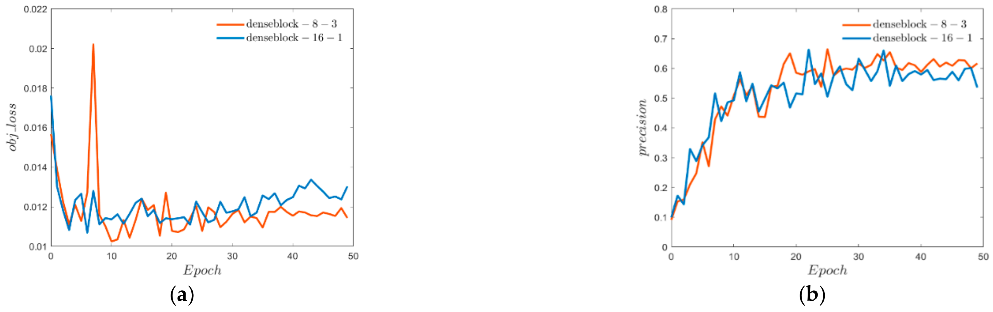
4.2. Experiments with Dense Convolutional Networks (DenseBlock)

In the experiment, first, the parameter adjustment experiment is carried out for each improved module in the text, and then a single improved network is compared with YOLOv5s. Finally the improved modules are synthesized and compared with the original network and the current mainstream target detection network.

4.2.1. Experimental Parameters

Under the dataset, optimize the parameter settings of the DenseBlock module, i.e., Grow_rate and layers. Grow_rate represents how many feature layers are connected to the previous feature layer and how many are connected to the back. The layers represent how many DenseBlock dense link layers are used.

The DenseBlock module has the characteristics of the number of input channels and parameter settings that determine the number of output channels, so there are two sets of parameter settings for matching the number of channels before and after the experiment, as shown in

Table 2. DenseBlock module experimental parameter table.

Parameter Settings	8-3	16-1
Training times	100	100
Recognition rate(mAP)	0.616	0.602
Model size(mb)	14.43	14.43
Inference time(ms)	4.8	4.5

.

4.2.2. Training Results

The training results for different parameter selections are shown in Figure 7.

From Figure 7a, it can be seen that the target loss value of the 8-3 experimental group is lower than that of the 16-1 experimental group. That is, the target anchor frame classification is more accurate, and from Figure 7b,d, it can be seen that the detection accuracy of the 8-3 experimental group in the first 20 epochs is lower than that of the 16-1 experimental group, but with the increase of the number of trainings. When the epoch reaches more than 40 times and the experimental result tends to stabilize, the detection accuracy of the 8-3 experimental group is higher. As can be seen from Figure 7c, there is no significant difference in recall rates.

For the parameter growth_rate and num_layers used in the DenseBlock module, due to the limitation of input and output channels, a total of 2 parameter combinations were used for comparative experiments. It can be seen that under the premise of the same model size, the DenseBlock module with more dense layers and lower learning rate has an obvious performance advantage, but it is worth mentioning that the training time of adding the DenseBlock module is longer, the training configuration requirements are higher, and the amount of computation is greater.

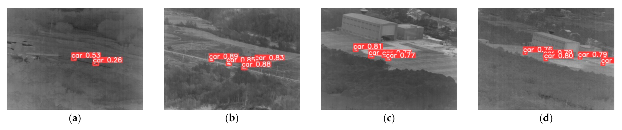
4.2.3. Testing Results

The detection results before and after adding the DenseBlock module are shown in Figure 8, Figure 9 and Figure 10.

As can be seen from Figure 8, Figure 9 and Figure 10, whether the 8-3 experimental group or the 16-1 experimental group, the average confidence in detecting infrared small target vehicles is higher than that of the original algorithm, and the experimental group of 8-3 performed better than the experimental group of 16-1. This shows that the DenseBlock module with 8-3 parameters is more suitable for the detection of this dataset, and this parameter group is used in the comprehensive module of subsequent experiments.

4.3. Experiments with End-Side Neural Networks (GhostNet)

4.3.1. Experimental Parameters

According to the feature map redundancy of the Ghost convolutional layer, it can be inferred that the deep feature map is not suitable for feature redundancy inference by using linear calculation. Therefore, the replaced convolutional layers are close to the input layer, which are the backbone network convolutional layers. The parameter settings such as the number of Ghost convolutional layers replaced, training time, and recognition rate in the experiment are shown in

Table 3. Ghost module experimental parameter table.

Ghost Convolutional Replacement Quantity	1	2	3	4
Training times	100	100	100	100
Recognition rate(mAP) Model size(mb)	0.64	0.655	0.613	0.599
	14.05	13.99	13.71	12.57
Inference time(ms)	4.2	4.3	4.4	4.4

.

4.3.2. Training Results

The training results for different parameter selections are shown in Figure 11.

From Figure 11a, it can be seen that the Ghost experimental group replacing the two convolution layers had lower target loss values during training, and it can be seen from Figure 11b that the detection accuracy of the 4-2 experimental group was higher in the 30 epochs after the training results tended to stabilize. From Figure 11c,d, it can be seen that the recall rate and detection accuracy of the 4-2 experimental group in a total of 100 epoch training are always higher than that of other experimental groups, and the gap is noticeable.

For a single Ghost module, although the model size is effectively reduced with the increase of the number of substitutions, after replacing three ordinary convolution layers, the recognition rate shows a downward trend. That is, too much feature map redundancy harms the detection accuracy, and in terms of model size and inference time, the more Ghost convolutional replacements, the smaller the model, and the slower the inference time.

When replacing two convolution layers, the network recognition rate shows a peak due to the increase of the redundancy feature map, which proves that the redundancy of the feature map is not always positive for the recognition rate, at the same time, the inference time is faster, and the model size increases less. It is the best choice to replace the two convolution layers, so the subsequent Ghost modules use a replacement number of two Ghost convolutional modules by default.

4.3.3. Testing Results

After adding the corresponding Ghost module, the test result is shown in Figure 12.

From the comparison of Figure 8 and Figure 12, it can be seen that the network that joins the Ghost convolution can accurately detect the vehicle target, and the detection accuracy has been improved in each scene. Among the two targets in scene 1, the detection accuracy was the highest, increasing by 26% and 50% respectively.

4.4. Experiments with the Squeeze-and-Excitation Layer (SE Layer)

In the SE layer, the module position of the SE layer is optimized by parameter reduction, and the more suitable module position and parameters have been pre-selected according to the previous experiments. See

Table 4. SE module experimental parameter table.

Module Position and Parameters	Before SPPF	After SPPF	Reduction = 16	Reduction = 4
Training times	50	50	50	50
Recognition rate (mAP) Model size (mb)	0.661	0.655	0.612	0.667
	14.67	14.67	14.67	14.47
Extrapolation time (ms)	4.5	4.4	4.4	4.4

for experimental parameters.

4.4.1. Training Results

The training results for different parameter selections are shown in Figure 13 and Figure 14.

From Figure 13a, it can be seen that the target loss value is higher when the reduction parameter is taken with reduction = 16. From Figure 13b–d, it can be seen that the totality is relatively stable after 40 epochs, and the experimental group with a parameter of 16 has a higher detection accuracy. As can be seen from Figure 14a,b, the target loss values of the two experimental control groups are similar. The detection accuracy is generally similar. As can be seen from Figure 14c,d, the overall mAP value of the target detection in the pre-SPPF experimental group was higher due to the higher recall rate in the pre-SPPF experimental group.

In terms of attention parameters, try where different SE layers are added, and finally select SPPF before and after doing the comparison experiment. It can be seen that the SE module is more suitable before the SPPF, according to the analysis of the role of SPPF can be obtained. The SE module for the high-level features of the channel attention mechanism is more biased toward the image features before the pooling layer rather than the semantic features after the pooling layer. At the same time, according to the comparison of reduction parameters, the SE model with a reduction of 4 performs prominently in a single epoch but is not stable overall, whereas the overall trend results with a parameter of 16 perform better. That is to say, increasing the decline rate of the hidden layer channel can improve the detection rate of the image attention mechanism. Finally, the parameter reduction of 16 is selected according to the image.

4.4.2. Testing Results

When the SE module is added to the SPPF and the reduction parameter is selected 16, the detection results are shown in Figure 15.

Compared with Figure 8 and Figure 15, the average detection accuracy of the network with the addition of an attention mechanism is significantly improved in each scene.

4.5. Experiments with EIOU

For the replacement loss function, because YOLOv5 used a total of GIOU, DIOU, and CIOU, three kinds of loss functions, along with the development of the loss function research, now YOLOv5 mainly uses CIOU. This article uses EIOU to replace CIOU. For improved models, replacement loss function increases the detection recognition rate, so the subsequent experiments are all replaced with EIOU loss functions. Training results are shown in Figure 16 below.

As can be seen from Figure 16, compared with CIOU, the recall value increases and the object loss value decreases in the detection results by using EIOU, and the mAP value of the EIOU group in the overall model detection is significantly improved.

5. Modular Combination Improved Algorithm Experiment

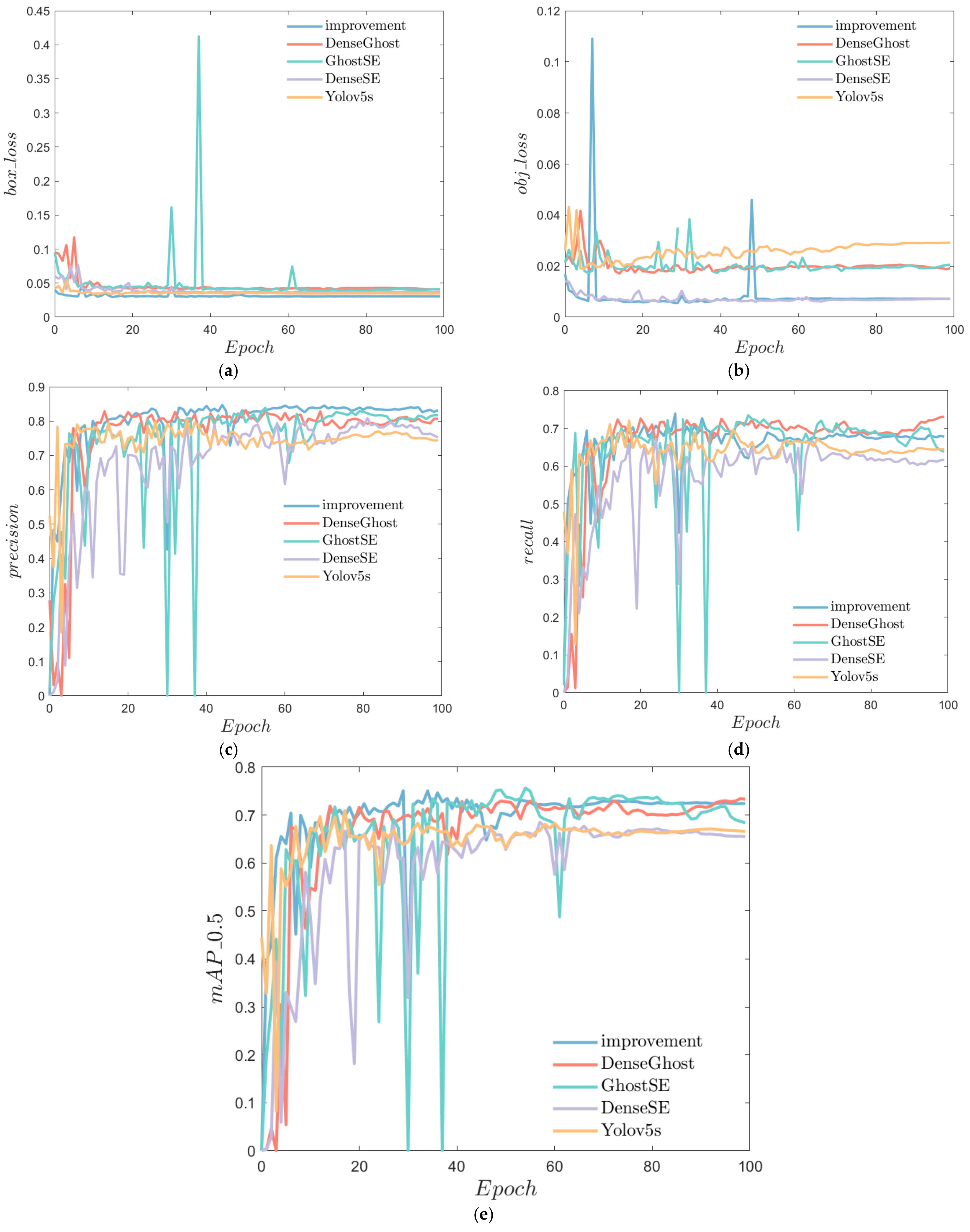
5.1. Improved YOLOv5 Network Experiment

In order to improve the detection effect of the comprehensive improved model, the single module is compared, and they are added to the original YOLOv5 algorithm in pairs. The results are shown in

Table 5. Comparison table of results for individual module.

Improved Modules	YOLOv5s	Ghost Convolution	DenseBlock	SE Module
Number of trainings	100	100	100	100
Recognition rate(mAP)	0.685	0.650	0.713	0.660
Model size(mb)	14.07	13.99	14.43	14.67
Extrapolation time(ms)	4.2	4.3	4.8	4.4

and

Table 6. Comparison table of results for the synthesis improved module.

Network Structure	YOLOv5s	Dense + Ghost + SE	Dense + Ghost	Ghost + SE	Dense + SE
Number of trainings	100	100	100	100	100
Recognition rate(mAP)	0.685	0.731	0.73	0.753	0.685
Model size(mb)	14.07	14.80	14.36	14.59	15.15
Extrapolation time(ms)	4.2	8.5	5.0	4.5	8.6

. Refer to [24,25] for a graphical representation of the optimization results. Convert the mAP column in Table 5 to a histogram as Figure 17 shows and convert the mAP column in Table 6 to a histogram as Figure 18 shows.

5.1.1. Training Results

Figure 16 shows the comparison between the detection accuracy of the DenseBlock, Ghost convolution and SE modules and the detection accuracy of the original YOLOv5 algorithm.

The characteristics and applicable scenes of each module can be drawn from Figure 19, and from Figure 19a, the confidence loss of the DenseBlock module is significantly lower than that of other modules. That is, the module is more effective in improving the detection accuracy and stability of the target. As can be seen from Figure 19b,c, although the SE module can improve the recognition accuracy, it will lead to a decrease in the recall rate; from Figure 19d, when used alone, the DenseBlock module has the most obvious improvement, but the mAP value of Ghost convolution and SE module does not improve significantly. A combination of these modules and the comprehensive improvement comparison chart is shown in Figure 20.

As can be seen from Figure 20a,b, the target loss value and anchor-frame loss value after the combination of DenseBlock, Ghost Convolution and SE module are the lowest. As can be obtained from Figure 20c, the accuracy of the three module combinations is also the highest. In Figure 20d, although the recall rate after the combination of DenseBlock, Ghost convolution, and SE module is not the highest. It has the smallest fluctuation after 40 epochs and is more stable. As can be seen from Figure 20e, although the mAP value is not significantly improved when using the Ghost convolution and SE module alone, the combined effect is obvious. There is a mutual inhibition effect between the DenseBlock module and the SE module, resulting in no obvious difference between the superimposed effect of the two and the original algorithm. From the analysis of the module principle, SE is a hybrid single-layer, multi-channel information feature used to improve the detection ability. At the same time, the use of the DenseBlock module with multiple feature layers in series makes the feature complexity increase instead of decrease, reducing the detection accuracy. Compared with other improvements, the comprehensive improvement in detection ability has improved the detection stability, while maintaining the lowest target loss value and the best detection effect. However, in some cases where the model detection speed is required to be high, or the size and computing power of the model are limited by the installed equipment, using the Ghost + SE improvement module with similar comprehensive improvement effect may be an option.

5.1.2. Testing Results

The results of the improved network for infrared vehicle target detection are shown in Figure 21, Figure 22, Figure 23, Figure 24 and Figure 25.

It can be seen from Figure 21, Figure 22, Figure 23, Figure 24 and Figure 25 that for the two small targets in scene 1, the detection accuracy of Dense + Ghost is improved by 18% and 46%, respectively, compared with the original YOLOv5. Dense + SE is improved by 16% and 43%, respectively, and Dense + Ghost is respectively improved by 18% and 46%. Dense + Ghost is improved by 20% and 51%, and Dense + Ghost + SE is improved by 18% and 52%, respectively. In the objectives of scene 2 and scene 3, the combination of the two modules is improved compared to the original YOLOv5, and the detection effect of the Dense + Ghost + SE combination is not much different from that of the two combinations. At the same time, in scene 4, the Dense + Ghost + SE modules detect the target vehicle that is not detected by other modules. In general, the Dense + Ghost + SE modules combination has better detection performance for small targets, and has a higher probability to detect targets that could not be found in the previous network due to low accuracy.

6. Conclusions

The article analyzes the characteristics of infrared vehicle images, starting from the four improvement modules of DenseBlock, Ghost Convolution, SE Module, and EIOU. The original YOLOv5 network is improved, and experiments are carried out on the effect of each module. The advantages and disadvantages of each module are analyzed, and the two combinations are compared and analyzed, and the following conclusions are drawn:

• When the module is used alone, the accuracy of DenseBlock and EIOU modules are significantly improved, and the Ghost convolution and SE modules are not significantly improved, which is almost the same as the original network, or even lower.
• When the module is used in combination, in addition to the combination of DenseBlock module and SE module, the other combinations have obvious improvement effects. When using three modules at the same time, the target loss value is the lowest, the accuracy rate is the highest, and the mAP value is the most stable.
• For a small target with occlusion, whether it is the original YOLOv5 or the two–two combination module, it has not been detected, and the phenomenon of missed detection has occurred. When using three modules at the same time, the occlusion targets can be effectively detected, and the rate of missed detection can be reduced.
• When using the improved algorithm in this paper, the insertion-extraction module can be adjusted according to different task requirements. For example, the DenseBlock module can be added to the detection target requiring higher stability. If a higher detection probability is required, the SE module can be added to the neck layer of the improved network. If higher detection speed is required, DenseBlock or SE module can be removed.

Combined with the experimental results and conclusions, the next steps are clarified:

• Although the missed target is detected, the confidence is not high, and the network needs to be further optimized.
• In the actual scene, the infrared vehicle target is not only interfered by the background of vegetation, buildings, etc., but also by smoke and electromagnetic interference, resulting in the degradation of the image quality. How to extract the vehicle target in the complex interference environment is a challenge for future work.

References

1. Kim, J.; Hong, S.; Baek, J.; Lee, H. Autonomous vehicle detection system using visible and infrared camera. In Proceedings of the 2012 12th International Conference on Control, Automation and Systems, Jeju, Korea, 17–21 October 2012; pp. 630–634. [Google Scholar]
2. Chen, D.; Jin, G.; Lu, L.; Tan, L.; Wei, W. Infrared Image Vehicle Detection Based on Haar-like Feature. In Proceedings of the 2018 IEEE 3rd Advanced Information Technology, Electronic and Automation Control Conference (IAEAC), Chongqing, China, 12–14 October 2018; pp. 662–667. [Google Scholar]
3. Liu, Y.; Su, H.; Zeng, C.; Li, X. A Robust Thermal Infrared Vehicle and Pedestrian Detection Method in Complex Scenes. Sensors 2021, 21, 1240. [Google Scholar] [CrossRef] [PubMed]
4. Iwasaki, Y.; Kawata, S.; Nakamiya, T. Vehicle detection even in poor visibility conditions using infrared thermal images and its application to road traffic flow monitoring. In Emerging Trends in Computing, Informatics, Systems Sciences, and Engineering; Springer: New York, NY, USA, 2013; pp. 997–1009. [Google Scholar]
5. Tang, T.; Zhou, S.; Deng, Z.; Zou, H.; Lei, L. Vehicle detection in aerial images based on region convolutional neural networks and hard negative example mining. Sensors 2017, 17, 336. [Google Scholar] [CrossRef] [PubMed] [Green Version]
6. Liu, X.; Yang, T.; Li, J. Real-time ground vehicle detection in aerial infrared imagery based on convolutional neural network. Electronics 2018, 7, 78. [Google Scholar] [CrossRef] [Green Version]
7. Ouyang, L.; Wang, H. Vehicle target detection in complex scenes based on YOLOv3 algorithm. IOP Conf. Ser. Mater. Sci. Eng. 2019, 569, 052018. [Google Scholar] [CrossRef]
8. Li, L.; Yuan, J.; Liu, H.; Cao, L.; Chen, J.; Zhang, Z. Incremental Learning of Infrared Vehicle Detection Method Based on SSD. In Proceedings of the 2020 IEEE 20th International Conference on Communication Technology (ICCT), Nanning, China, 28–31 October 2020; pp. 1423–1426. [Google Scholar]
9. Mahmood, M.T.; Ahmed, S.R.A.; Ahmed, M.R.A. Detection of vehicle with Infrared images in Road Traffic using YOLO computational mechanism. IOP Conf. Ser. Mater. Sci. Eng. 2020, 928, 022027. [Google Scholar] [CrossRef]
10. Zhu, Z.; Liu, Q.; Chen, H.; Zhang, G.; Wang, F.; Huo, J. Infrared Small Vehicle Detection Based on Parallel Fusion Network. Acta Photonica Sin. 2022, 51, 0210001. [Google Scholar]
11. Redmon, J.; Divvala, S.; Girshick, R.; Farhadi, A. You Only Look Once: Unified, Real-Time Object Detection. In Proceedings of the 2016 IEEE Conference on Computer Vision and Pattern Recognition (CVPR), Las Vegas, NV, USA, 27–30 June 2016; pp. 779–788. [Google Scholar] [CrossRef] [Green Version]
12. Zhang, X.; Zhu, X. Vehicle Detection in the aerial infrared images via an improved YOLOv3 network. In Proceedings of the 2019 IEEE 4th International Conference on Signal and Image Processing (ICSIP), Wuxi, China, 19–21 July 2019; pp. 372–376. [Google Scholar]
13. Li, Z.; Zhou, F. FSSD: Feature fusion single shot multibox detector. arXiv 2017, arXiv:1712.00960. [Google Scholar]
14. Redmon, J.; Farhadi, A. Yolov3: An incremental improvement. arXiv 2018, arXiv:1804.02767. [Google Scholar]
15. Han, J.; Liao, Y.; Zhang, J.; Wang, S.; Li, S. Target Fusion Detection of LiDAR and Camera Based on the Improved YOLO Algorithm. Mathematics 2018, 6, 213. [Google Scholar] [CrossRef] [Green Version]
16. Deng, Z.; Yang, R.; Lan, R.; Liu, Z.; Luo, X. SE-IYOLOV3: An Accurate Small Scale Face Detector for Outdoor Security. Mathematics 2020, 8, 93. [Google Scholar] [CrossRef] [Green Version]
17. Zhang, X.; Zhu, X. Moving vehicle detection in aerial infrared image sequences via fast image registration and improved YOLOv3 network. Int. J. Remote Sens. 2020, 41, 4312–4335. [Google Scholar] [CrossRef]
18. Wang, Z.; Wu, L.; Li, T.; Shi, P. A Smoke Detection Model Based on Improved YOLOv5. Mathematics 2022, 10, 1190. [Google Scholar] [CrossRef]
19. Kasper-Eulaers, M.; Hahn, N.; Berger, S.; Sebulonsen, T.; Myrland, Ø.; Kummervold, P. Short Communication: Detecting Heavy Goods Vehicles in Rest Areas in Winter Conditions Using YOLOv5. Algorithms 2021, 14, 114. [Google Scholar] [CrossRef]
20. Wu, W.; Liu, H.; Li, L.; Long, Y.; Wang, X.; Wang, Z. Application of local fully Convolutional Neural Network combined with YOLO v5 algorithm in small target detection of remote sensing image. PLoS ONE 2021, 16, e0259283. [Google Scholar] [CrossRef] [PubMed]
21. The Third “Aerospace Cup” National Innovation and Creativity Competition Preliminary Round, Proposition 2, Track 2, Optical Target Recognition, Preliminary Data Set. Available online: https://www.atrdata.cn/#/customer/match/2cdfe76d-de6c-48f1-abf9-6e8b7ace1ab8/bd3aac0b-4742-438d-abca-b9a84ca76cb3?questionType=model (accessed on 15 March 2022).
22. Jiang, B.; Ma, X.; Lu, Y.; Li, Y.; Feng, L.; Shi, Z. Ship detection in spaceborne infrared images based on Convolutional Neural Networks and synthetic targets. Infrared Phys. Technol. 2019, 97, 229–234. [Google Scholar] [CrossRef]
23. Shi, M.; Wang, H. Infrared Dim and Small Target Detection Based on Denoising Autoencoder Network. Mob. Netw. Appl. 2020, 25, 1469–1483. [Google Scholar] [CrossRef]
24. Alrasheedi, A.F.; Alnowibet, K.A.; Saxena, A.; Sallam, K.M.; Mohamed, A.W. Chaos Embed Marine Predator (CMPA) Algorithm for Feature Selection. Mathematics 2022, 10, 1411. [Google Scholar] [CrossRef]
25. Sharma, A.K.; Saxena, A. A demand side management control strategy using Whale optimization algorithm. SN Appl. Sci. 2019, 1, 870. [Google Scholar] [CrossRef] [Green Version]
Figure 1. Dataset partial image example. (a) Single target. (b) Multi-target. (c) Single target in complex environment. (d) Multi-target in complex environment.
Electronics 11 02344 g001
Figure 2. Image Characteristic analysis. (a) Original image. (b) 3D grayscale plot. (c) Grayscale histogram. (d) Original image in complex environment. (e) 3D grayscale plot. (f) Grayscale histogram.
Electronics 11 02344 g002
Figure 3. Schematic diagram of the DenseBlock structure.
Electronics 11 02344 g003
Figure 4. Schematic diagram of Ghost convolutional structure.
Electronics 11 02344 g004
Figure 5. Schematic diagram of the structure of the SE layer.
Electronics 11 02344 g005
Figure 6. Improved YOLOv5 network.
Electronics 11 02344 g006
Figure 7. Comparison results of DenseBlock parameters. (a) Target loss. (b) Accuracy rate. (c) Recalling rate. (d) mAP value.
Electronics 11 02344 g007aElectronics 11 02344 g007b
Figure 8. YOLOv5s detection map. (a) Scene 1. (b) Scene 2. (c) Scene 3. (d) Scene 4.
Electronics 11 02344 g008
Figure 9. 8-3 DenseBlock detection results. (a) Scene 1. (b) Scene 2. (c) Scene 3. (d) Scene 4.
Electronics 11 02344 g009
Figure 10. 16-1 DenseBlock detection results. (a) Scene 1. (b) Scene 2. (c) Scene 3. (d) Scene 4.
Electronics 11 02344 g010
Figure 11. Comparison of the number of GhostConv replacements. (a) Confidence loss. (b) Accuracy rate. (c) Recalling rate. (d) mAP value.
Electronics 11 02344 g011aElectronics 11 02344 g011b
Figure 12. Ghost convolutional test results. (a) Scene 1. (b) Scene 2. (c) Scene 3. (d) Scene 4.
Electronics 11 02344 g012
Figure 13. SE reduction parameter comparison results. (a) Target loss. (b) Accuracy rate. (c) Recalling rate. (d) mAP value.
Electronics 11 02344 g013
Figure 14. SE module position comparison result. (a) Target loss. (b) Accuracy rate. (c) Recalling rate. (d) mAP value.
Electronics 11 02344 g014
Figure 15. SE layer detection results. (a) Scene 1. (b) Scene 2. (c) Scene 3. (d) Scene 4.
Electronics 11 02344 g015
Figure 16. EIOU detection results. (a) Target loss. (b) Accuracy rate. (c) Recalling rate. (d) mAP value.
Electronics 11 02344 g016
Figure 17. Single-module mAP histogram.
Electronics 11 02344 g017
Figure 18. Comprehensive improvement of mAP histogram.
Electronics 11 02344 g018
Figure 19. Comparison of results of single-module training. (a) Target loss. (b) Accuracy rate. (c) Recalling rate. (d) mAP value.
Electronics 11 02344 g019
Figure 20. Comprehensive improvement comparison chart. (a) Target loss. (b) Anchor-frame loss; (c) Accuracy rate. (d) Recalling rate. (e) mAP value.
Electronics 11 02344 g020
Figure 21. YOLOv5 detection map. (a) Scene 1. (b) Scene 2. (c) Scene 3. (d) Scene 4.
Electronics 11 02344 g021
Figure 22. Dense + Ghost detection diagram. (a) Scene 1. (b) Scene 2. (c) Scene 3. (d) Scene 4.
Electronics 11 02344 g022
Figure 23. Dense + SE detection diagram. (a) Scene 1. (b) Scene 2. (c) Scene 3. (d) Scene 4.
Electronics 11 02344 g023
Figure 24. Dense + Ghost detection diagram. (a) Scene 1. (b) Scene 2. (c) Scene 3. (d) Scene 4.
Electronics 11 02344 g024
Figure 25. Dense + Ghost + SE detection diagram. (a) Scene 1. (b) Scene 2. (c) Scene 3. (d) Scene 4.
Electronics 11 02344 g025