Article

Recognition of Emotion with Intensity from Speech Signal Using 3D Transformed Feature and Deep Learning

1
Department of Computer Science and Engineering, Khulna University of Engineering & Technology, Khulna 9203, Bangladesh
2
Graduate School of Science and Technology, Gunma University, Kiryu 376-8515, Japan
*
Authors to whom correspondence should be addressed.
Electronics 2022, 11(15), 2362; https://doi.org/10.3390/electronics11152362
Submission received: 15 June 2022 / Revised: 15 July 2022 / Accepted: 25 July 2022 / Published: 28 July 2022
(This article belongs to the Section Computer Science & Engineering)

Abstract

:
Speech Emotion Recognition (SER), the extraction of emotional features with the appropriate classification from speech signals, has recently received attention for its emerging social applications. Emotional intensity (e.g., Normal, Strong) for a particular emotional expression (e.g., Sad, Angry) has a crucial influence on social activities. A person with intense sadness or anger may fall into severe disruptive action, eventually triggering a suicidal or devastating act. However, existing Deep Learning (DL)-based SER models only consider the categorization of emotion, ignoring the respective emotional intensity, despite its utmost importance. In this study, a novel scheme for Recognition of Emotion with Intensity from Speech (REIS) is developed using the DL model by integrating three speech signal transformation methods, namely Mel-frequency Cepstral Coefficient (MFCC), Short-time Fourier Transform (STFT), and Chroma STFT. The integrated 3D form of transformed features from three individual methods is fed into the DL model. Moreover, under the proposed REIS, both the single and cascaded frameworks with DL models are investigated. A DL model consists of a 3D Convolutional Neural Network (CNN), Time Distribution Flatten (TDF) layer, and Bidirectional Long Short-term Memory (Bi-LSTM) network. The 3D CNN block extracts convolved features from 3D transformed speech features. The convolved features were flattened through the TDF layer and fed into Bi-LSTM to classify emotion with intensity in a single DL framework. The 3D transformed feature is first classified into emotion categories in the cascaded DL framework using a DL model. Then, using a different DL model, the intensity level of the identified categories is determined. The proposed REIS has been evaluated on the Ryerson Audio-Visual Database of Emotional Speech and Song (RAVDESS) benchmark dataset, and the cascaded DL framework is found to be better than the single DL framework. The proposed REIS method has shown remarkable recognition accuracy, outperforming related existing methods.

1. Introduction

Speech is the most popular way to communicate with others in daily life and is largely used for emotional expression [1]. Speech can carry two types of information, literal information and relative information [2]. The literal information highlights direct meaning, and relative information means the implicit messages such as emotion contained in the speech [3]. Speech is always a potential source of the emotional state of a person. In the computational intelligence or machine learning (ML) domain, Speech Emotion Recognition (SER) is known as the task of determining and classifying the emotional features of speech.
SER has consistently faced challenging ML issues due to the complexity of speech signals [2]. SER has two distinct steps: feature extraction from the speech signal and emotion classification. The efficiency of emotional features obtained from speech significantly impacts SER performance [3]. Various DL models based on neural networks have been investigated for SER [4], which include Deep Belief Networks (DBN) [3], Convolutional Neural Network (CNN) [1,4], Recurrent Neural Network (RNN) [5] and Long Short-Term Memory (LSTM) network [5]. Prominent existing methods employ different feature extraction and signal transformation methods on speech signals, and then DL methods are applied to the transformed signal for emotion classification.
A remarkable observation from the existing SER studies is those only considered emotion categorization from speech signals regardless of the intensity that belongs to it [6]. Emotion intensity (e.g., Normal, Strong) for a particular emotional expression (e.g., sad, angry) has a crucial impact. In case of being very sad/angry, a person may fall into serious disruptive activity. In some cases, strong-disgusting activity is the pre-action towards the suicidal event. Today, online broadcasts from mentally upset persons through social media while performing a disgusting activity have increased. Such online demonstrations draw negative attention from society, and action to resolve such issues is crucially vital for the well-being of society. Therefore, automatic emotion recognition with its level of intensity is a very important timely demand issue that is the primary concern of this study.
Recognition of emotion and its intensity from speech (REIS), employing transformation of the speech signals and the appropriate DL models, is the central contribution of this study. A significant aspect of this investigation is the simultaneous utilization of three different transformations of speech signals, using Mel-frequency Cepstral Coefficient (MFCC), Short-time Fourier Transform (STFT), and Chroma STFT. Integrating transformed features from three individual methods constitutes 3D structural features that are fed into the DL model for emotion extraction and classification. Particularly, two different DL frameworks are investigated in the proposed REIS: (i) a single DL framework for the simultaneous classification of emotion with intensity and (ii) a cascaded DL framework, where the task is performed in two successive stages. In the cascaded DL framework, the 3D transformed signal is classified into emotion categories using a DL model (in Stage 1) and then recognized its intensity level using another DL model (in Stage 2). Each DL model consists of a 3D CNN, Time Distribution Flatten (TDF) layer, and Bidirectional LSTM (Bi-LSTM) network. The 3D CNN block extracts convolved features from 3D transformed speech. The convolved features are flattened through the TDF layer and then fed into Bi-LSTM to classify emotion with intensity in a single DL framework. In the cascaded framework, a DL model (similar to the single DL framework) is used for emotion classification in the first stage and then intensity measure in the second stage with another DL model. The proposed REIS has been investigated on the benchmark speech data source, and the cascaded DL framework significantly achieved better performance over the single DL framework. The proposed method also outperformed related existing methods. At a glance, the transformation of the speech signal into 3D form and the deployment of cascaded DL framework for classification are the significant two-fold contributions of this study to the well-performed emotion recognition with intensity level.
The rest of the paper is written as follows. Section 2 reviews several existing SER studies related to this study. Section 3 presents the proposed REIS describing individual components. Section 4 presents experimental outcomes and an evaluation of the proposed model on a benchmark dataset. Finally, Section 5 concludes the paper with a few observations.

2. Literature Review

SER is a trending research area introduced two decades ago [7]. Several innovative strategies have been introduced to enhance the performance of SER. The two fundamental phases of SER are feature extraction and emotion classification. In the feature extraction phase, it can be a manually created feature or a learned feature using DLs [8,9]. Additionally, classification can be carried out using ML, e.g., DL. A review of the background methods is included in Appendix A, which provides the basics of the related ML schemes for a better understanding of the novelty and contributions of the proposed method.

2.1. SER with Machine Learning (ML)

Pioneer SER methods are investigated using traditional ML algorithms [7], including Random Forest (RF) [10], Decision Tree (DT) [11], Naïve Bayes (NB) [12], Support Vector Machines (SVM) [13], Hidden Markov Model (HMM) [14], K-Nearest Neighbors (K-NN) [15] and Gradient Boosting Classifier [16]. Several modified ML models are also observed for SER, which shows better performance than the traditional model [17]. The Ensemble Random Forest to Trees (ERF-Trees) [11] algorithm was introduced to extract essential emotion features from a small dataset. The algorithm combines the advantages of RF and DT by reducing the limitations and error rates of those traditional algorithms separately.
The Hybrid of Grey Wolf Optimizer (HGWO) [15] strategy was adopted with the NB classifier to overcome the limitation of the traditional NB. At some points, the conventional NB finds the wrong prediction. To overcome the limitations, HGWO finds optimized weights for the NB, potentially reducing the error rate compared to the traditional approach. The Multi-layer Hybrid Fuzzy SVM (MLHF-SVM) [18] model was founded on sub-classification and classification. In the model, Fuzzy C-means with the Inertia Weight Particle Swarm Optimization (FCM-IEPSO) algorithm was implemented to cluster the speech feature into sub-class to improve the performances of final classification using multi-layer SVM.
Some other recent ML algorithms for SER are wavelet packet transform (WPT) cochlear filter bank and RF classifier [10], Golden Ratio Based Equilibrium Optimization (GREO) algorithm [14], and Agent ML [19], etc.

2.2. SER with Deep Learning (DL) and Signal Transformation

Recently, DL-based approaches have been shown to perform well in SER tasks, where embedded feature extraction in DL methods is a significant property for better performance. Based on the input signals, the DL-based methods may be categorized into two terms: raw speech signals and transformed speech signals. Using raw speech signals, Zhao et al. [20] introduced a 1D CNN-LSTM network for SER. Latif et al. [21] also employed several DL models on raw speech. Several modified DL models are also observed for SER, including capsule neural network [22], 3D CNN-LSTM model [10], 3D CNN using k-means clustering [8], 2D CNN with a self-attention dilated residual network [9], Spiking Neural Network (SNN) [23], convolutional capsule (Conv-Cap) and bi-directional gated recurrent unit (Bi-GRU) [24], attention-LSTM-attention [25], Bi-GRU with attention mechanism [26], CNN with a capsule neural network (Caps Net) [13], temporal CNN with self-attention transfer network (SATN) [27], 1D CNN based on the multi-learning trick (MLT) [14], cascaded denoising CNN (Dn-CNN) [28], and a pre-trained deep CNN model with attention [29]. The learning features are the main attraction of different DL-based SER methods.
Several DL models with transformed speech features are investigated for SER for better recognition performance. Chen et al. [30] investigated a Deep CNN model containing two CNN blocks with two fully connected (FC) layers. Each CNN block contains a convolution layer (CL), ReLU activation layer, and max-pooling layer [20]. The first block CL contains 128 feature maps, and the second block CL contains 64 future maps. Each feature map uses a 5 × 5 kernel size with a single stride, and the max-pooling layer holds a 2 × 2 kernel with two strides. Finally, two FC layers were connected with the soft-max classifier. Mustaqeem and Kwon [4] introduced a model with seven CNN FB and an FC layer with soft-max activation. Every FB of the model has a CL layer, a BN layer, and ELU activation. The kernel size for the first CL was 7 × 7, the second CL layer was 5 × 5, and the last five CLs were 3 × 3. Zhao et al. [20] proposed a hybrid CNN-LSTM model with four CNN feature blocks (FB) with a single LSTM. Each FB contains a CL, an ELU activation layer, a batch normalization (BN) layer, and a max-pooling layer. The first two CLs used 64 feature maps, and the rest of the two CLs used 128 feature maps. All the feature maps contain the same kernel size three with one stride. On the other hand, only the first max-pooling layer holds two kernels with two strides. Each of the other pooling layers contains four kernels with four strides. The output of the fourth FB was flattened to connect with an LSTM layer. Sultana et al. [31] recently investigated a hybrid model with a Deep CNN and a Bi-LSTM [31] network with a TDF layer. The model consists of four FBs, and each block has a CL, a BN, a ReLU activation layer, and a max-pooling layer. The first two CL blocks contain 64 feature maps, and the last two CL blocks contain 128 feature maps.

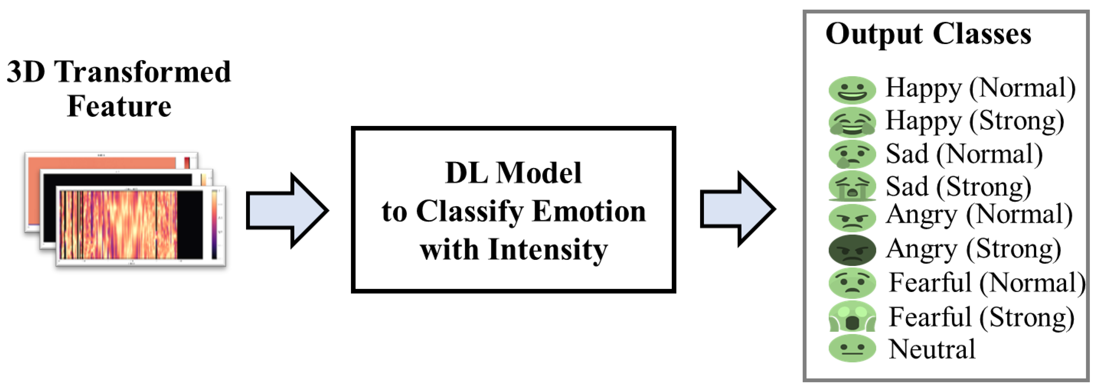
3. Recognition of Emotion and Its Intensity from Speech (REIS) Method

Speech is the most common mode of communication in live media, including Facebook, YouTube, and other voice communication networks or platforms, which often contain individual emotions. Identifying the extreme level of emotion (e.g., very sad or very angry) is often crucial to prevent individuals from taking disruptive action, including suicidal or devastating movements, which may also impact our society. Once such a destructive and intense emotion is detected, an alarm or notification may be forwarded to the supportive unit about the person to take necessary action(s). Figure 1 illustrates such a computational intelligence-based supportive conceptual framework, which automatically filters out the disruptive activities from speech signals in live media with the aim of the society’s welfare against critical issues. In the framework, the automatic filtering of the speech signal by recognizing emotion and its intensity from speech (REIS) is the most challenging task that is addressed in this study.
Figure 2 depicts the proposed REIS system by mentioning fundamental phases of speech signal processing, signal transformation, feature extraction, and emotion categorization. The speech signal is the input of REIS, and emotion categorization with intensity is the output of the system. Suppose input speech signals are for four emotional categories (Happy, Sad, Angry, and Fearful) and samples for Neutral. Based on intensity, individual emotions are labeled as Normal and Strong. Therefore, the proposed REIS categorizes the speech samples into nine classes: Happy (Normal), Happy (Strong), Sad (Normal), Sad (Strong), Angry (Normal), Angry (Strong), Fearful (Normal), Fearful (Strong), and Neutral. In the proposed REIS system, speech signal transformation and classification with DL are the two crucial tasks, as explained below.
For the speech signal transformation, to generate features appropriate for the DL model to recognize emotion from it, three popular signal transformation methods are considered in this study: MFCC [1], STFT [2], and Chroma STFT [32]. The speech signal operation using a method (e.g., MFCC, STFT) produces a two-dimensional (2D) transformed feature. This study integrates three different same-sized 2D features as a 3D transformed feature. The set of different features in an integrated way provides better emotional attributes than individuals [8,33]. This 3D transformed feature is considered as the input of 3D CNN of the DL classifier model to recognize emotion.
A DL model extracts features through several embedded layers before finally classifying them into emotion categories. An appropriate DL model must be selected for adequately classifying emotion with intensity level from the transformed 3D feature. In the proposed study, two DL-based frameworks are investigated to find the effective one for REIS. The first one is a single DL framework for the classification of emotion with intensity together, and the second one is the cascaded DL framework that performs the task in two different stages. Figure 3 illustrates the single DL framework to classify the 3D transformed features into emotions with the intensity level, i.e., nine classes: Happy (Normal), Happy (Strong), Sad (Normal), Sad (Strong), Angry (Normal), Angry (Strong), Fearful (Normal), Fearful (Strong), and Neutral. Figure 4 illustrates the cascaded DL framework. In the first stage, Figure 4a, the input 3D transformed features are classified into five classes: Happy, Sad, Angry, Fearful, and Neutral. In the second stage, Figure 4b, the intensity of the recognized emotion in Stage 1 is identified with a different DL model. Notably, the same 3D feature is used as input for Stage 2, but distinct DL models are used to measure the intensity of individual emotion cases. For example, if a sample is classified as Sad in Stage 1, a particular and specialized DL model for Sad will be used to measure its intensity.
Two different DL-based frameworks (i.e., single and cascaded) hold significant distinct properties. The single DL framework is simple and easy to understand as only one DL model classifies emotion with intensity. However, the emotion classification and intensity measure tasks of the single DL model seem relatively complex. On the other hand, the whole task (emotion classification with intensity) is sub-divided into emotion classification and intensity measures, which are performed by two different DL models in a cascaded framework. Such sub-division simplifies the task for DL models to perform better in classification.
A DL model extracts features through several embedded layers and finally classifies them into predefined categories. In the proposed REIS, the categories to be classified are emotion with intensity (in single DL framework), emotion (in Stage 1 of cascaded DL framework), and intensity measure (in Stage 2 of cascaded DL framework). All three DL models use 3D transformed features as input; therefore, essential operations in the initial stages of the models are the same. The three DL models are significantly different in the number of classes and tasks to be performed. For simplicity, the same DL architecture is applied for all three DL models for a varying number of output classes. Specifically, this study investigates a DL model with CNN and LSTM, the most popular DL models, for REIS.
Figure 5 illustrates the DL model architecture for REIS, consisting of 3D CNN and Bi-LSTM. As REIS uses 3D transformed features, the 3D CNN is the most suitable for feature extraction. On the other hand, Bi-LSTM is considered due to its capability to handle sequential data and its performance in recent studies [34,35]. Figure 5a shows the basic structure of the proposed DL architecture having four 3D CNN feature blocks (FB) and Bi-LSTM with a TDF layer. Figure 5b illustrates the structure of CNN FB, where each FB consists of a 3D convolutional layer, a batch normalization (BN) layer, a ReLU layer, and a 3D max-pooling layer. The output of the convolved FB is put into a TDF layer. The TFD layer flattens the FB, which is the input to Bi-LSTM. The outcome of the Bi-LSTM layer is fed to a fully connected (FC) to recognize emotion or intensity level.
Table 1 shows layer parameters for the proposed 3D CNN Bi-LSTM architecture, where the convolutional layer of FB-1 and FB-2 has 64 filters, and the FB-3 and FB-4 have 128 filters. All the convolutional layers have the same 3 × 3 × 3 kernels and 1 × 1 × 1 strides. The max-pooling layers have a kernel size of 2 × 2× 1, and the stride size is 2 × 2 × 1 for FB-1. However, the last three FB max-pooling layers have a kernel of size 4 × 4 × 1 and a stride size of 4 × 4 × 1. The output of the FB-4 is 1 × 4 × 3 sized 128 maps which are fed into a TDF layer. The TFD layer flattens the FB-4 output to 1536 features (=1 × 4 × 3 × 128), which is the input to Bi-LSTM. The outcome of the Bi-LSTM layer is 512 features fed to an FC layer. This final layer is fed to the Softmax layer, which computes output probabilities for all the classes. The number of neurons in the output layer depends on where to use DL and its purpose. The number of neurons will be nine for the single DL framework. For the cascaded DL framework, there will be five and two neurons in the DL models in Stage 1 and Stage 2, respectively.
The complete 3D CNN Bi-LSTM model is trained to minimize the categorical cross-entropy loss function. The cross-entropy function is a commonly used loss function for the multi-class classification problem [36]. As emotion recognition in this study is a multi-class classification problem, the cross-entropy loss function is considered like other studies [37]. The cross-entropy function calculates the Loss by computing the following equation.
L o s s = i = 1 T o t a l   I n s t a n c e s   S i z e y i   ·   l o g   y ^ i
Here, y i     and   t is the target value and total instances, respectively, in the model output. The minus sign ensures that the Loss becomes smaller when the distributions become closer to each other.

4. Experimental Studies

The proposed REIS was evaluated on a benchmark speech dataset and the performance was compared with other related methods. The following subsections provide details about the dataset, experimental setup, outcomes, and performance comparison.

4.1. Benchmark Dataset and Experimental Setup

The RAVDESS dataset, an audio-visual resource for American-English emotional speech and songs [38], was considered to evaluate the proposed REIS. Twelve males and twelve females carried out the recording of stimuli. The dataset included 1440 speech files for eight emotion categories and 1012 song files for six emotion categories [38]. In this study, samples of five common categories (i.e., neutral and four emotion categories) from speech and song were merged and considered to evaluate REIS. Each emotional expression was further split into two levels of emotional intensity (Normal, Strong). Such intensity markers allow the evaluation of REIS. Finally, on the intensity basis, each of the four emotional categories was subdivided into Normal (for Normal) and Strong (for Strong) categories. Finally, the task of the RAVDESS dataset was used to classify the samples into nine classes: Neutral, Happy (Normal), Happy (Strong), Sad (Normal), Sad (Strong), Angry (Normal), Angry (Strong), Fearful (Normal), and Fearful (Strong). Each class holds 188 audio samples, and there were a total of 1692 (=188 × 9) samples.
The dataset was divided into training and test sets in an around 80:20 ratio by collecting samples from each of the nine categories. The training set, including 1350 (=150 × 9) samples, was used to train the model, and the test set with the remaining 342 (=38 × 9) samples was reserved to evaluate the generalization ability of the model after training. Notably, the RAVDESS dataset is used in several studies, including several recent ones [8,39,40]. However, all the existing studies consider emotion classification only, without considering the emotional intensity issue. The proposed REIS is the first attempt to classify emotion with intensity.
The speech signal transformation was performed using the python Librosa library [41]. Speech signals in the RAVDESS dataset are around five seconds long with a sample rate of 48 kHz [38], and to make such signals compatible with DL input, signals are resampled to a 16 kHz sample rate and equal eight seconds long by padding with null values. Therefore, all the signals were equally reformed as 128,000 (=8 × 16,000) bit-vectors that were transformed by the individual methods. Figure 6 shows MFCC, STFT, and Chroma STFT transformed features for a sample speech signal. In processing MFCC, 250 hop lengths and 128 sequences were considered. Thus, the MFCC feature in Figure 6a are with 128 sequences and 512 (i.e., 128,000/250) frames. In the STFT set, the hop length was also 250, and the FFT window length was 256. So, the resulting STFT feature was also 128 (=256/2) sequences and 512 frames, which is shown in Figure 6b. Figure 6c is the Chroma STFT feature with the same size as STFT. After that, the transformed features were integrated into the 3D transformed feature using NumPy library [42] with sizes 128 × 512 × 3 and fed into the DL model.
The development of the DL models was carried out with python open source DL libraries, Keras [43] and Tensorflow [44]. The model began with a 3D convolution layer with an input size the same as the integrated 3D transformed feature. The 3D convolution layers have four parameters, filter size, kernel size, strides size, and padding. However, the 3D max-pooling layers have two parameters: kernel size and stride size. Layer parameters are shown in Table 1. The TFD layer flattens the FB-4 output to 1536 features (=1 × 4 × 3 × 128), the input to Bi-LSTM. The outcome of the Bi-LSTM layer was 512 features fed to an FC layer. This final layer was fed to the Softmax layer, which computes output probabilities for all the classes.
The experiments were carried out using a Jupyter notebook on the Google collab, which is a cloud-based GPU-enabled service [45]. Additionally, the local machine was an HP Pro-book notebook with an Intel Core i5-4200M @ 3.5 GHz processor, 16 GB RAM, and Intel HD Graphics 4200.

4.2. Experimental Results and Analysis

This section presents experimental outcomes on the RAVDESS dataset with both the DL frameworks. Loss and accuracy curves were developed and analyzed for insightful evaluation of the proposed method. Finally, the performance of the proposed method was compared with existing methods.

4.2.1. Outcomes of Single DL Framework

Figure 7 presents the loss and accuracy curves for training and test sets while training epochs vary up to 70. It is notable from Figure 7a that the training set loss curve smoothly reduced and reached close to zero after 40 epochs. On the other hand, the test set loss curve decreased initially, and after 30 epochs, it did not reduce but fluctuate. The training and test set curve patterns are acceptable in the machine learning concept as the training set is used to update the model, and the test set is used to measure the performance only. Accuracy curves in Figure 7b reflect the recognition proficiency for the corresponding loss curves shown in Figure 7a. Training set accuracy improved smoothly and reached 100%, while Loss was close to zero at around training epoch 40. The best test set accuracy was also achieved at this point.
Test set accuracy is the primary concern for the performance measure of any machine learning model. Table 2 shows the confusion matrix of the test set samples at the best-performed point. In the table, the total test samples of individual categories are distributed into truly classified numbers and misclassified into other classes by the trained model. It has already been mentioned that every emotion category (except Normal) holds Normal and Strong intensity categories. When a sample is misclassified in a different emotion category, it is counted in category miss. If a sample is misclassified in the emotion intensity measure, it is counted in intensity miss. For example, for 38 Neutral samples, a total of 32 are genuinely classified as Neutral; the remaining six samples are in the category miss for misclassification as Happy and Sad. The model showed the best performance for Angry (Strong), having three intensity miss cases, and it showed the worst performance for Sad (Strong), misclassifying seven samples in category miss and seven other samples in intensity miss. Again, the misclassification of Fearful as Sad was also remarkable as Fearful emotion was nearly compatible with Sad. At a glance, a total of 73 (=46 + 27) test samples were missed out of 342 test instances, and, therefore, the test set accuracy was 78.65% (i.e., (342 − 73) × 100/342) for emotion recognition with intensity by the single DL framework.

4.2.2. Outcomes of Cascaded DL Framework

The task of REIS is performed in a cascaded DL framework in two different stages. A DL model in Stage 1 classifies samples into emotional categories, which were trained with 1350 (= 150 × 9) training samples. Figure 8 presents the Loss and Accuracy curves for both training and test sets while training epochs vary up to 45. Training set loss curve smoothly reduced and reached close to zero after 25 epochs, as shown in Figure 8a. On the other hand, the test set loss curve was initially reduced, and after 20 epochs, it did not reduce. Training set accuracy improved smoothly and reached 100%, while Loss was close to zero around training epoch 25, as seen in Figure 8b. The best test set accuracy was also achieved at this point. A total of 34 test samples were missed (i.e., category miss) in this stage. Therefore, emotion category classification accuracy on the test set was 90.06% (i.e., (342 − 34) × 100/342). Table 3 shows the confusion matrix of the test set samples for a better understanding. The truly classified 308 samples were considered to measure intensity in Stage 2.
In Stage 2, four different DLs were considered to measure the intensity of individual emotions (i.e., Happy, Sad, Angry, and Fearful). Each DL model is trained with 300 samples for a particular emotion, i.e., 150 samples for Normal and 150 samples for Strong. Figure 9 shows the loss plots of training and test sets of four different emotions in this stage, and Figure 10 shows the corresponding accuracy plots. In this stage, the task was binary classification into Normal and Strong intensity categories. Therefore, accuracies were shown to be relatively stronger, even in the case of the test set.
The samples classified in Stage 1 were then used to measure the respective emotional intensity in Stage 2 with the DL model for individual categories. For example, 76 Fearful test samples were classified in Stage 1 into Fearful, Sad, and Happy classes, with the number of cases 64, 9, and 3, respectively. Therefore, three different DLs are used to measure the intensity of samples of three emotion categories. Table 4 shows the test set confusion matrix of the cascaded DL framework. The intensity levels of 34 missed samples in Stage 1 were also clarified in the table. For example, a total of nine Fearful samples misclassified as Sad (shown in Table 3 for Stage 1) are from the Normal and Strong categories in numbers 5 and 4, respectively. The five Fearful (Normal) samples are misclassified in intensity levels as Sad (Normal) for three cases and Sad (Strong) for two cases. The four Fearful (Strong) samples are misclassified as Sad (Normal) for three cases and Sad (Strong) for a single case. In Stage 2, the intensity measures of such a category of missed samples were unimportant because those are always counted into the category miss cases.
On the other hand, intensity measure in Stage 2 for truly classified samples in Stage 1 is an essential issue in the cascaded DL framework in REIS. For example, the total truly classified sad samples are 71 in Stage 1, which belongs to Normal and Strong intensity cases as 35 and 36, respectively. In Stage 2, truly classified in intensity measure for Sad (Normal) and Sad (Strong) are 32 and 35, respectively. Therefore, the intensity miss count for Sad (Normal) and Sad (Strong) are three and one, respectively. Out of 308 truly classified samples in Stage 1, the total intensity miss count for four emotion categories was only 12, i.e., 296 samples were truly classified in the intensity measure case. In total, 46 (=34 + 12) samples were misclassified by the cascaded DL framework and showed overall classification accuracy of 87.71% (i.e., (342 − 46) × 100/342). The achieved accuracy was better than the single DL framework described in the previous section.

4.2.3. Performance Comparison between the Single DL and Cascaded DL Frameworks

This section presents an overall performance comparison between single DL and cascaded DL frameworks on REIS. This time, a 4-fold cross-validation procedure was followed by the available RAVDESS dataset with 1692 samples to evaluate both DL frameworks. For four independent experiments in 4-fold cross-validation, 423 (=47 × 9), different samples were considered as the test set by turn, and 1269 (=1692 − 423 = 47 × 3 × 9) samples were used to train the DL models. Table 5 compares the REIS performance (i.e., Test Set Accuracy) of the single DL and cascaded DL frameworks. The outcomes for four individual experiments (i.e., Folds) are also included in the table for better observation. In any case, the cascaded DL framework was found to be better than the single DL framework. For example, using Fold 1 with the single DL, the total category miss and intensity miss are 61 and 34, respectively. Since the truly classified samples are 328, the resulting accuracy stands at 77.54% (=328 × 100/423). For the same fold, the numbers of the category miss and intensity miss are lower for the cascaded DL framework, and the values are 48 and 18, respectively, which correspond to the resulting accuracy of the cascaded DL framework being 84.40%. Finally, 4-fold cross-validation accuracy (average of four individual folds) for the single DL and cascaded DL frameworks are 76.66% and 85.34%, respectively, which supports the proficiency of the cascaded DL framework.

4.3. Performance Comparison with Existing Methods

This study performed recognition of emotion with its intensity from speech (i.e., REIS). Several DL-based studies are available on speech emotion recognition (i.e., SER) only, where the intensity issue of emotion is ignored. Two different frameworks and DL model selection are the key elements of this study. At first, the performance of the proposed DL model was compared to the state-of-the-art methods for SER. The performance of REIS was compared by conducting experiments in two frameworks for this study.
Table 6 compares the SER performance (i.e., Test Set Accuracy) of the proposed REIS framework with state-of-the-art on the RAVDESS dataset. The outcome of the test set emotion classification accuracy from Stage 1 of the cascaded DL framework (Section 4.2.2) was considered for this comparison. The accuracy of the existing methods is the reported results in [31], which are also on the test set with 20% reserved samples. Here, we also compared feature transformation and classification methods of the individual methods. Existing methods considered different DL models for classification from Log-Mel spectrums transformation of speech signals in 2D form. The proposed method used 3D transformed features integrating MFCC, STFT, and Chroma STFT features. Regarding DL model architecture, the proposed model is similar to [31], having CNN, TDF, and LSTM, but the 3D CNN model is considered in the proposed method to make it compatible with 3D transformed input feature. The proposed method achieved an accuracy of 90.06%, whereas the recent model of [31] is the best among the existing methods and shows an accuracy of 82.69%. Feature enhancement and appropriate DL-model in the proposed model gave a remarkable performance concerning the existing methods.
Table 7 compares the REIS performance (i.e., Test Set Accuracy from Section 4.2.1 and Section 4.2.2) of the proposed REIS with two investigated frameworks of this study with state-of-the-art on the RAVDESS dataset. The experimental results for the proposed REIS are discussed in the experimental outcome section. On the other hand, the results for the existing methods are the outcomes of the experiment conducted on corresponding models following similar investigations of the proposed REIS in single DL and cascaded DL frameworks. Therefore, the test set accuracy presented in the table is the same for the 20% reserved test samples for individual methods. It is remarkable from the table that a cascaded DL framework is better than a single DL framework for any method. For example, the method with CNN [30] showed an accuracy of 33.91% only in the single DL framework and an accuracy of 71.05% in the cascaded framework. It is also remarkable from the table that the proposed REIS is better than any other existing method, showing less category miss and fewer intensity miss counts. The proposed method achieved the best accuracy of 87.71% with the cascaded DL framework, whereas the recent model of [31] is the best among the existing methods and shows an accuracy of 81.28%. Finally, the proposed cascaded framework with the 3D transformed feature-based DL model appeared to be the best-suited method for emotion recognition with intensity, i.e., REIS.

5. Conclusions

This study addressed the recognition of emotion with intensity from speech (i.e., REIS), a new and stimulating enthusiasm for SER, which can automatically detect and filter disruptive activities in online media and be used in emerging social applications. Specifically, speech emotion recognition with intensity is explored through the 3D transformation of the speech signals and the use of appropriate DL frameworks. Besides the pioneering intensity-based emotion identification, the present study confirmed significant achievements in the technical development of effective learning from speech data. Experimental studies have demonstrated that the speech signal transformed into 3D form integrating three different 2D transformations enhances features for better identifiability. Moreover, the proposed DL framework with 3D CNN and Bi-LSTM ensures better recognition performance. The cascaded DL framework, which recognizes emotion and its intensity in two different stages, is the best-suited method for the proposed REIS system. The recognition accuracy is as high as 87.71% for 342 test samples, despite the model being trained with only 1350 samples. The performance of the proposed REIS is compared with several state-of-the-art methods to evaluate and confirm its superiority over the other methods.
Several future research scopes have emerged from the present study. Instead of using the same DL models in the cascaded DL framework, it is worth investigating more specific DL architectures for emotion recognition (in Stage 1) and intensity measures (in Stage 2). Furthermore, other than the three prominent speech signal transformations (i.e., MFCC, STFT, Chroma STFT), new signal transformation techniques can be used to explore multi-dimensional transformed features. Such extended studies might be interesting to apply to other speech datasets to realize higher recognition accuracy.

Author Contributions

Conceptualization, M.R.I. and M.A.H.A.; Formal analysis, M.R.I. and M.A.H.A.; Funding acquisition, M.A.S.K.; Investigation, M.R.I. and M.A.H.A.; Software, M.R.I.; Supervision, M.A.S.K.; Writing—original draft, M.R.I.; Writing—review and editing, M.A.H.A., M.A.S.K. and K.Y. All authors have read and agreed to the published version of the manuscript.

Funding

This research received no external funding.

Conflicts of Interest

The authors declare no conflict of interest.

Appendix A. Review of Background Methods

With machine learning or the DL model, speech signal processing and emotion recognition are the two basic functional steps of any SER system. Existing methods used several speech transformation methods and different DL models. The fundamentals of several speech transformation methods and DL models are described briefly to ensure the paper is self-contained.

Appendix A.1. Speech Signal Processing and Transformation

The success of any ML-based SER model relies heavily on appropriate speech transformation. The correct transformation may result in a better model, but the incorrect features undermine the training process [8]. Briefly, descriptions of three considered signal transformations (i.e., MFCC, STFT, and Chroma STFT) are given to better comprehend the proposed SER system.
MFCC is a well-known sound processing method through the representation of the short-term power spectrum of a sound. Figure A1 presents the MFCC method consisting of the signal, applying discrete furrier transformation (DFT), taking a log of magnitude on the Mel scale, and then reversing the discrete cosine transform (DCT) [1],
M F C C i = φ N cos ( i ( φ 1 ) π N ) i = 1 , 2   128
Figure A1. Steps of MFCC Process.
Electronics 11 02362 g0a1
The STFT is a Fourier-related transform for identifying the sinusoidal frequency and phase content of individual signal portions (e.g., sound) as they change frequently, where an audio sound x is defined as,
S T F T x [ n , k ] = m = n n + ( N 1 ) x [ m ] e j   2 π k N m
In Equation (A2), n   and   k represent the time and frequency of a signal, respectively, where, k = 0 ,   1 ,   ,   N 1 . At a given time n, the STFT relates to the FFT of the sequence from samples   x [ n ]   to   x [ n + ( N 1 ) ] . Consequently, one technique of calculating the STFT is to use the N number of FFT processors simultaneously [2].
The Chroma value of audio represents the intensity of the twelve distinctive pitch classes. The fundamental approach of Chroma STFT is to integrate all spectral (e.g., STFT) information relating to a specific pitch class into a single factor [32].
C ( m , c ) = { p [ 0 : 127 ]   | p   m o d   12 = c } y L F ( m , p )
In Equation (A3), given a pitch-based log-frequency spectrogram   y L F : Z × [ 0 :   11 ]     R 0 can be calculated by adding all pitch coefficients from the same Chroma.

Appendix A.2. Deep Learning Models

Neural network-based DL models have been investigated in recent SER studies. Among different DL models, CNN [1,4], and LSTM network [5] are the base of the proposed SER model. CNN is the most well-known DL architecture motivated by natural creatures’ basic visual attention mechanism [4]. Figure A2 shows a CNN’s basic architecture consisting of convolutional layers, pooling layers, and fully connected layers. The convolution layer is made up of multiple convolution kernels that are used to generate various feature maps. Each neuron in a feature map and is linked to a neighboring neuron in the previous layer.
Figure A2. Fundamental Structure of a CNN.
Electronics 11 02362 g0a2
The basic structure the convolution layer takes to transform feature x ( i , j , k ) as input, and the result z   ( i ,   j ,   k ) is calculated by convolving the input data with the dimension of convolution kernel w ( i ,   j ,   k ) of size a × b × c .
z ( i , j , k ) = x ( i , j , k ) w ( i , j , k ) = q = a a r = b b s = c c x ( q , r , s )   ·   w ( i q ,   j r ,   k s )
The BN layer, which normalizes the activations of the previous layer at each batch, obtains the results [46].
z i l = b i l + j z i l 1   ·   w i j l
Here, z i l and z i l 1 denote the i th output feature on the l th layer and the j th input feature at the ( l 1 ) th layer; w i j l represents the convolution kernel between the i th   and   j th feature. The layer applies a transformation that keeps the convolved features, average close to zero and their variance close to one based on each batch sample shown in Equation (A6),
Z i l = B N ( z i l ) = γ ( z i l μ σ 2 + ε ) + β
µ   and   σ 2 describe the mean and variance of the output feature at the i th output at the l th layer. ε   and   β explain the learnable parameters to highlight the expressive power of the networks. The activation function is the rectified linear unit (ReLU) layer, which is utilized to address the gradient vanishing and exploding issues. In the ReLU layer, the method is given to Equation (A7).
f ( x ) = max ( 0 , x )
When the normalized output is less than zero, it changes to zero. Otherwise, the output remains the same as the input. The features are sent to the max-pooling layer, which conducts a non-linear down-sampling function on the features and minimizes their resolution. The layer’s properties can be expressed as follows,
Z k l = m a x p Ω k Z p l
where Ω k is the pooling region with index ,   Z k l , and Z p l , which are the features of the output and input of the l th max-pooling layer with index k   and   p .
The LSTM is a kind of RNN made up of recurrently associated memory blocks, including memory cells with self-connections that record the network’s temporal states [5]. It is mainly effective in learning sequential data in the form of time steps. Here, Figure A3 presents the architecture of an LSTM cell.
Figure A3. Basic Architecture of an LSTM Cell.
Electronics 11 02362 g0a3
Hence, z t l 1 is input, and z t l is the output of LSTM that can be expressed by Equations (A9)–(A13),
f t = σ g ( W f z t l 1 + U f z t 1 l + b f )
i t = σ g ( W i z t l 1 + U i z t 1 l + b i )
o t = σ g ( W o z t l 1 + U o z t 1 l + b o )
c t = f t °   c t 1 + i t °   σ c ( W c z t l 1 + U c z t 1 l + b c )
z t l = o t ° σ z c t
Here,   f t , i t , and   o t   in Equations (A9)–(A11) are gate vectors; σ g is a sigmoid function; σ c   and   σ z are tangents; script i ,   o ,   f ,   c in Equations (A9)–(A12) all are used to indicate the gates of input, output, forget, and cell; sign ° represents the Hadamard product [20]. However, LSTM has limitations in terms of the learning formulation from earlier time scales and can only learn in one direction, whereas Bi-LSTM can access relevant information in both forward and reverse directions. The Bi-LSTM method, an updated model of LSTM, helps to understand the context and eliminate the ambiguity from the samples [3]. Bi-LSTM uses two hidden layers in the same output layer to learn both forward ( z t = z 1   ,   z 2   , z 3   ,   z n   ) and backward ( z t = z 1 , z 2 , z 3   z n ) sequence data. The final output of this cell y t   is formed by both z t   and z t the final sequence of outlooks such as y = ( y 1 ,   y 2 ,   y 3 , y t ,   y n ) [47], shown in Figure A4.
Figure A4. Basic Architecture of a Bi-LSTM.
Electronics 11 02362 g0a4

References

  1. Sahidullah, M.; Saha, G. Design, analysis and experimental evaluation of block based transformation in MFCC computation for speaker recognition. Speech Commun. 2012, 54, 543–565. [Google Scholar] [CrossRef]
  2. Garrido, M. The Feedforward Short-Time Fourier Transform. IEEE Trans. Circuits Syst. II Express Briefs 2016, 63, 868–872. [Google Scholar] [CrossRef]
  3. Angadi, S.; Reddy, V.S. Hybrid deep network scheme for emotion recognition in speech. Int. J. Intell. Eng. Syst. 2019, 12, 59–67. [Google Scholar] [CrossRef]
  4. Mustaqeem; Kwon, S. A CNN-assisted enhanced audio signal processing for speech emotion recognition. Sensors 2020, 20, 183. [Google Scholar] [CrossRef] [PubMed]
  5. Das, R.K.; Islam, N.; Ahmed, M.R.; Islam, S.; Shatabda, S.; Islam, A.K.M.M. BanglaSER: A speech emotion recognition dataset for the Bangla language. Data Brief 2022, 42, 108091. [Google Scholar] [CrossRef] [PubMed]
  6. Zhang, H.; Xu, M. Weakly Supervised Emotion Intensity Prediction for Recognition of Emotions in Images. IEEE Trans. Multimed. 2021, 23, 2033–2044. [Google Scholar] [CrossRef]
  7. Nakatsu, R.; Solomides, A.; Tosa, N. Emotion recognition and its application to computer agents with spontaneous interactive capabilities. In Proceedings of the 1999 IEEE Third Workshop on Multimedia Signal Processing (Cat. No.99TH8451), Copenhagen, Denmark, 13–15 September 1999; Volume 2, pp. 804–808. [Google Scholar] [CrossRef]
  8. Atila, O.; Şengür, A. Attention guided 3D CNN-LSTM model for accurate speech based emotion recognition. Appl. Acoust. 2021, 182, 108260. [Google Scholar] [CrossRef]
  9. Zhao, Z.; Li, Q.; Zhang, Z.; Cummins, N.; Wang, H.; Tao, J.; Schuller, B.W. Combining a parallel 2D CNN with a self-attention Dilated Residual Network for CTC-based discrete speech emotion recognition. Neural Netw. 2021, 141, 52–60. [Google Scholar] [CrossRef]
  10. Hamsa, S.; Shahin, I.; Iraqi, Y.; Werghi, N. Emotion Recognition from Speech Using Wavelet Packet Transform Cochlear Filter Bank and Random Forest Classifier. IEEE Access 2020, 8, 96994–97006. [Google Scholar] [CrossRef]
  11. Rong, J.; Li, G.; Chen, Y.P.P. Acoustic feature selection for automatic emotion recognition from speech. Inf. Process. Manag. 2009, 45, 315–328. [Google Scholar] [CrossRef]
  12. Ramesh, S.; Gomathi, S.; Sasikala, S.; Saravanan, T.R. Automatic speech emotion detection using hybrid of gray wolf optimizer and naïve Bayes. Int. J. Speech Technol. 2021, 1–8. [Google Scholar] [CrossRef]
  13. Milton, A.; Sharmy Roy, S.; Tamil Selvi, S. SVM Scheme for Speech Emotion Recognition using MFCC Feature. Int. J. Comput. Appl. 2013, 69, 34–39. [Google Scholar] [CrossRef]
  14. Dey, A.; Chattopadhyay, S.; Singh, P.K.; Ahmadian, A.; Ferrara, M.; Sarkar, R. A Hybrid Meta-Heuristic Feature Selection Method Using Golden Ratio and Equilibrium Optimization Algorithms for Speech Emotion Recognition. IEEE Access 2020, 8, 200953–200970. [Google Scholar] [CrossRef]
  15. Lanjewar, R.B.; Mathurkar, S.; Patel, N. Implementation and comparison of speech emotion recognition system using Gaussian Mixture Model (GMM) and K-Nearest Neighbor (K-NN) techniques. Procedia Comput. Sci. 2015, 49, 50–57. [Google Scholar] [CrossRef]
  16. Sun, C.; Tian, H.; Chang, C.-C.; Chen, Y.; Cai, Y.; Du, Y.; Chen, Y.-H.; Chen, C.C. Steganalysis of Adaptive Multi-Rate Speech Based on Extreme Gradient Boosting. Electronics 2020, 9, 522. [Google Scholar] [CrossRef]
  17. Arya, R.; Pandey, D.; Kalia, A.; Zachariah, B.J.; Sandhu, I.; Abrol, D. Speech based Emotion Recognition using Machine Learning. In Proceedings of the 2021 IEEE Mysore Sub Section International Conference (MysuruCon), Hassan, India, 24–25 October 2021; pp. 613–617. [Google Scholar] [CrossRef]
  18. Huang, S.; Dang, H.; Jiang, R.; Hao, Y.; Xue, C.; Gu, W. Multi-layer hybrid fuzzy classification based on svm and improved pso for speech emotion recognition. Electronics 2021, 10, 2891. [Google Scholar] [CrossRef]
  19. Kim, D.H.; Nair, S.B. Novel emotion engine for robot and its parameter tuning by bacterial foraging. In Proceedings of the 2009 5th International Symposium on Applied Computational Intelligence and Informatics, Imisoara, Romania, 28–29 May 2009; pp. 23–27. [Google Scholar] [CrossRef]
  20. Zhao, J.; Mao, X.; Chen, L. Speech emotion recognition using deep 1D & 2D CNN LSTM networks. Biomed. Signal Process. Control 2019, 47, 312–323. [Google Scholar] [CrossRef]
  21. Latif, S.; Rana, R.; Khalifa, S.; Jurdak, R.; Epps, J. Direct modelling of speech emotion from raw speech. In Proceedings of the 20th Annual Conference of the International Speech Communication Association: Crossroads of Speech and Language (INTERSPEECH 2019), Graz, Austria, 15–19 September 2019; pp. 3920–3924. [Google Scholar] [CrossRef]
  22. Van, L.T.; Nguyen, Q.H.; Le, T.D.T. Emotion recognition with capsule neural network. Comput. Syst. Sci. Eng. 2022, 41, 1083–1098. [Google Scholar] [CrossRef]
  23. Gavrilescu, M.; Vizireanu, N. Feedforward neural network-based architecture for predicting emotions from speech. Data 2019, 4, 101. [Google Scholar] [CrossRef]
  24. Maji, B.; Swain, M.; Mustaqeem. Advanced Fusion-Based Speech Emotion Recognition System Using a Dual-Attention Mechanism with Conv-Caps and Bi-GRU Features. Electronics 2022, 11, 1328. [Google Scholar] [CrossRef]
  25. Yu, Y.; Kim, Y.J. Attention-LSTM-Attention model for speech emotion recognition and analysis of IEMOCAP database. Electronics 2020, 9, 713. [Google Scholar] [CrossRef]
  26. Yan, Y.; Shen, X. Research on Speech Emotion Recognition Based on AA-CBGRU Network. Electronics 2022, 11, 1409. [Google Scholar] [CrossRef]
  27. Zhao, Z.; Bao, Z.; Zhang, Z.; Cummins, N.; Sun, S.; Wang, H.; Tao, J.; Schuller, B.W. Self-attention transfer networks for speech emotion recognition. Virtual Real. Intell. Hardw. 2021, 3, 43–54. [Google Scholar] [CrossRef]
  28. Nam, Y.; Lee, C. Cascaded convolutional neural network architecture for speech emotion recognition in noisy conditions. Sensors 2021, 21, 4399. [Google Scholar] [CrossRef]
  29. Zhang, H.; Gou, R.; Shang, J.; Shen, F.; Wu, Y.; Dai, G. Pre-trained Deep Convolution Neural Network Model with Attention for Speech Emotion Recognition. Front. Physiol. 2021, 12, 643202. [Google Scholar] [CrossRef] [PubMed]
  30. Chen, J.X.; Zhang, P.W.; Mao, Z.J.; Huang, Y.F.; Jiang, D.M.; Zhang, Y.N. Accurate EEG-Based Emotion Recognition on Combined Features Using Deep Convolutional Neural Networks. IEEE Access 2019, 7, 44317–44328. [Google Scholar] [CrossRef]
  31. Sultana, S.; Iqbal, M.Z.; Selim, M.R.; Rashid, M.M.; Rahman, M.S. Bangla Speech Emotion Recognition and Cross-Lingual Study Using Deep CNN and BLSTM Networks. IEEE Access 2022, 10, 564–578. [Google Scholar] [CrossRef]
  32. Ashraf, M.; Ahmad, F.; Rauqir, R.; Abid, F.; Naseer, M.; Haq, E. Emotion Recognition Based on Musical Instrument using Deep Neural Network. In Proceedings of the 2021 International Conference on Frontiers of Information Technology (FIT), Islamabad, Pakistan, 13–14 December 2021; pp. 323–328. [Google Scholar]
  33. Hajarolasvadi, N.; Demirel, H. 3D CNN-based speech emotion recognition using k-means clustering and spectrograms. Entropy 2019, 21, 479. [Google Scholar] [CrossRef]
  34. Mustaqeem; Kwon, S. MLT-DNet: Speech emotion recognition using 1D dilated CNN based on multi-learning trick approach. Expert Syst. Appl. 2021, 167, 114177. [Google Scholar] [CrossRef]
  35. Farooq, M.; Hussain, F.; Baloch, N.K.; Raja, F.R.; Yu, H.; Zikria, Y. Bin Impact of feature selection algorithm on speech emotion recognition using deep convolutional neural network. Sensors 2020, 20, 6008. [Google Scholar] [CrossRef]
  36. Zhou, Y.; Wang, X.; Zhang, M.; Zhu, J.; Zheng, R.; Wu, Q. MPCE: A Maximum Probability Based Cross Entropy Loss Function for Neural Network Classification. IEEE Access 2019, 7, 146331–146341. [Google Scholar] [CrossRef]
  37. Ando, A.; Mori, T.; Kobashikawa, S.; Toda, T. Speech emotion recognition based on listener-dependent emotion perception models. APSIPA Trans. Signal Inf. Process. 2021, 10, E6. [Google Scholar] [CrossRef]
  38. Livingstone, S.; Russo, F. The Ryerson Audio-Visual Database of Emotional Speech and Song (RAVDESS). PLoS ONE 2018, 13, e0196391. [Google Scholar] [CrossRef] [PubMed]
  39. Mustaqeem; Sajjad, M.; Kwon, S. Clustering-Based Speech Emotion Recognition by Incorporating Learned Features and Deep BiLSTM. IEEE Access 2020, 8, 79861–79875. [Google Scholar] [CrossRef]
  40. Tamulevičius, G.; Korvel, G.; Yayak, A.B.; Treigys, P.; Bernatavičienė, J.; Kostek, B. A study of cross-linguistic speech emotion recognition based on 2d feature spaces. Electronics 2020, 9, 1725. [Google Scholar] [CrossRef]
  41. McFee, B.; Raffel, C.; Liang, D.; Ellis, D.; McVicar, M.; Battenberg, E.; Nieto, O. Librosa: Audio and Music Signal Analysis in Python. In Proceedings of the 14th Python in Science Conference, Austin, TX, USA, 6–12 July 2015; pp. 18–24. [Google Scholar] [CrossRef]
  42. Van Der Walt, S.; Colbert, S.C.; Varoquaux, G. The NumPy array: A structure for efficient numerical computation. Comput. Sci. Eng. 2011, 13, 22–30. [Google Scholar] [CrossRef]
  43. Arnold, T.B. kerasR: R Interface to the Keras Deep Learning Library. J. Open Source Softw. 2017, 2, 296. [Google Scholar] [CrossRef]
  44. Abadi, M. TensorFlow: Learning functions at scale. ACM SIGPLAN Not. 2016, 51, 1. [Google Scholar] [CrossRef]
  45. Regis, F.; Alves, V.; Passos, R.; Vieira, M. The Newton Fractal’s Leonardo Sequence Study with the Google Colab. Int. Electron. J. Math. Educ. 2020, 15, em0575. [Google Scholar]
  46. Meng, H.; Yan, T.; Yuan, F.; Wei, H. Speech Emotion Recognition from 3D Log-Mel Spectrograms with Deep Learning Network. IEEE Access 2019, 7, 125868–125881. [Google Scholar] [CrossRef]
  47. Shahid, F.; Zameer, A.; Muneeb, M. Predictions for COVID-19 with deep learning models of LSTM, GRU and Bi-LSTM. Chaos Solitons Fractals 2020, 140, 110212. [Google Scholar] [CrossRef] [PubMed]
Figure 1. A supportive system framework through automatic filtering of disruptive activity from speech signal of live media.
Electronics 11 02362 g001
Figure 2. General architecture of proposed REIS approach.
Electronics 11 02362 g002
Figure 3. Single DL framework to classify emotion with intensity from 3D transformed speech signal.
Electronics 11 02362 g003
Figure 4. Cascaded DL framework to classify emotion and its intensity from 3D transformed speech signal in two different stages. (a) Stage 1: Classify emotion from 3D transformed feature; (b) Stage 2: Measure intensity for emotion classified in Stage 1.
Electronics 11 02362 g004
Figure 5. Deep learning architecture for proposed REIS. (a) Basic building block structure of the proposed DL architecture; (b) Structure of a convolutional feature block.
Electronics 11 02362 g005
Figure 6. Sample transformed feature of (a) MFCC (128 × 512), (b) STFT (128 × 512), and (c) Chroma STFT (128 × 512).
Electronics 11 02362 g006
Figure 7. Loss plot and accuracy plot of training and test sets of RAVDESS dataset for Single DL framework. (a) Loss vs. Training Epoch; (b) Accuracy vs. Training Epoch.
Electronics 11 02362 g007
Figure 8. Loss plot and accuracy plot of training and test sets of RAVDESS dataset for Stage 1 (Emotional Categorization) in Cascaded DL framework. (a) Loss vs. Training Epoch; (b) Accuracy vs. Training Epoch.
Electronics 11 02362 g008
Figure 9. Loss plot of training and test sets of four different emotions in RAVDESS dataset for Stage 2 (Intensity Measure) in Cascaded DL framework. (a) Happy Emotion; (b) Sad Emotion; (c) Angry Emotion; (d) Fearful Emotion.
Electronics 11 02362 g009
Figure 10. Accuracy plot of training and test sets of four different emotions in RAVDESS dataset for Stage 2 (Intensity Measure) in Cascaded DL framework. (a) Happy Emotion; (b) Sad Emotion; (c) Angry Emotion; (d) Fearful Emotion.
Electronics 11 02362 g010
Table 1. The layer parameters of the proposed 3D CNN Bi-LSTM architecture.
Feature Block (FB)Layer and TypeKernel SizeStride
Size
Input ShapeOutput Shape
FB-1Conv3D3 × 3 × 31 × 1 × 1128 × 512 × 3128 × 512 × 3 @ 64
Max-Pooling3D2 × 2 × 12 × 2 × 1128 × 512 × 3 @ 6464 × 256 × 3 @ 64
FB-2Conv3D3 × 3 × 31 × 1 × 164 × 256 × 3 @ 6464 × 256 × 3 @ 64
Max-Pooling 3D4 × 4 × 14 × 4 × 164 × 256 × 3 @ 6416 × 64 × 3 @ 64
FB-3Conv3D3 × 3 × 31 × 1 × 116 × 64 × 3 @ 6416 × 64 × 3 @ 128
Max-Pooling 3D4 × 4 × 14 × 4 × 116 × 64 × 3 @ 1284 × 16 × 3 @ 128
FB-4Conv3D3 × 3 × 31 × 1 × 14 × 16 × 3 @ 1284 × 16 × 3 @128
Max-Pooling 3D4 × 4 × 14 × 4 × 14 × 16 × 3 @ 1281 × 4 × 3 @ 128
TDF--1 × 4 × 3 @ 1281536
Bi-LSTM--1536512
FC--5129/5/2
Table 2. The test set confusion matrix by Single DL framework for emotion recognition with intensity level.
EmotionEmotion
Intensity
NeutralHappySadAngryFearfulCategory MissIntensity MissTotal
-NormalStrongNormalStrongNormalStrongNormalStrong
Neutral-32202200006038
HappyNormal12941000204438
Strong02310100045238
SadNormal20030310104338
Strong10172500237738
AngryNormal01400283016338
Strong00000335000338
FearfulNormal100360027210238
Strong00101113314338
Total=4627342
Table 3. Test set confusion matrix on emotion category in Stage 1 of Cascaded DL framework.
EmotionNeutralHappySadAngryFearfulCategory MissTotal
Neutral360200238
Happy368005876
Sad217102576
Angry141691776
Fearful0390641276
Total=34342
Table 4. The test set confusion matrix by the Cascaded DL framework for emotion recognition with intensity level.
EmotionEmotion
Intensity
NeutralHappySadAngryFearfulCategory MissIntensity MissTotal
-NormalStrongNormalStrongNormalStrongNormalStrong
Neutral-36002000002-38
HappyNormal13310000214138
Strong22320000114238
SadNormal11032300103338
Strong10013500102138
AngryNormal11110330105038
Strong02000135002138
FearfulNormal02132002738338
Strong00031001334138
Total=3412342
Table 5. The 4-fold cross-validation performance (i.e., test set accuracy) comparison between the Single DL and Cascaded DL Frameworks.
DL ModelSingle DL FrameworkCascaded DL Framework
Category MissIntensity MissAccuracy (%)Category MissIntensity MissAccuracy (%)
Fold 1613477.54481884.40
Fold 2753374.47491684.63
Fold 3583079.20401487.23
Fold 4743075.41471685.11
Average67.0031.7576.6646.0016.0085.34
Table 6. Performance (i.e., test set Accuracy) comparison with State-of-the-arts on emotion recognition.
Work Ref., YearFeature TransformationClassification ModelAccuracy (%)
Chen et al. [30], 2019Log-Mel spectrums2 CNN + 2 FC76.93
Zhao et al. [20], 2019Log-Mel spectrums4 CNN + LSTM77.96
Mustaqeem and Kwon [4], 2020Log-Mel spectrums7 CNN + 2 FC63.94
Sultana et al. [31], 2021Log-Mel spectrums4 CNN + TDF + Bi-LSTM82.69
Proposed Method (Stage 1 of Cascaded Framework)MFCC + STFT+ Chroma STFT4 3DCNN + TDF + Bi-LSTM90.06
Table 7. Performance (i.e., test set accuracy) comparison with State-of-the-arts for emotion recognition with intensity level.
Work Ref., YearFeature TransformationDL ModelSingle DL Framework Cascaded DL Framework
Category MissIntensity MissAccuracy (%)Category MissIntensity MissAccuracy (%)
Chen et al. [30], 2019Log-Mel spectrums2 CNN + 2 FC1943233.91772271.05
Zhao et al. [20], 2019Log-Mel spectrums4 CNN + LSTM572775.43512677.48
Mustaqeem and Kwon [4], 2020Log-Mel spectrums7 CNN + 2 FC862667.25692572.51
Sultana et al. [31], 2021Log-Mel spectrums4 CNN + TDF+ Bi-LSTM612176.02451981.28
Proposed REIS MFCC + STFT+ Chroma STFT4 3DCNN + TDF+ Bi-LSTM462778.65341287.71
Publisher’s Note: MDPI stays neutral with regard to jurisdictional claims in published maps and institutional affiliations.

