
Numerical Solution of the Poisson Equation Using Finite Difference Matrix Operators


Department of Electrical Engineering, Stanford University, Stanford, CA 94305, USA
Electronics 2022, 11(15), 2365; https://doi.org/10.3390/electronics11152365
Submission received: 21 June 2022
/
Revised: 24 July 2022
/
Accepted: 25 July 2022
/
Published: 28 July 2022
Abstract
:The Poisson equation frequently emerges in many fields of science and engineering. As exact solutions are rarely possible, numerical approaches are of great interest. Despite this, a succinct discussion of a systematic approach to constructing a flexible and general numerical Poisson solver can be difficult to find. In this introductory paper, a comprehensive discussion is presented on how to build a finite difference matrix solver that can solve the Poisson equation for arbitrary geometry and boundary conditions. The boundary conditions are implemented in a systematic way that enables easy modification of the solver for different problems. An image-based geometry-definition approach is also discussed. Python code of the numerical recipe is made publicly available. Numerical examples are presented that show how to set up the solver for different problems.
1. Introduction
The Poisson equation is an elliptical partial differential equation (PDE) and is ubiquitous in many areas of physics and engineering. Two of its common uses include modeling electrostatic potential and gravitational potential. Some forms of the Poisson equation also appear in fluid flow [1] and heat transfer problems [2,3]. Often, analytic solutions of such problems are not possible for cases of practical interest due to complex geometries. Numerically solving the Poisson equation is the only way to study these systems. As such, numerical solution methods for the Poisson equation are of significant interest [2,4,5].
There are several methods for solving the Poisson equation numerically [6]. The Finite-Difference Method (FDM) is one of the most simple and popular approaches [7,8,9,10]. This method involves replacing the continuous derivative operators with approximate, discrete finite-difference operators [11] that take the form of matrices. The method is intuitive and the solution process involves well-established linear algebraic methods. It suffers from some drawbacks, such as accurately representing complex geometries and boundaries. Methods such as the Finite Element Method (FEM) are better at handling arbitrary geometries. However, due to the ease of implementation and the intuitive nature of FDM, it remains a very popular approach for solving PDEs.
There are several references that discuss solving the Poisson equation using FDM [12]. While these papers cover many details, they usually do not present a systematic approach of constructing the numerical system (i.e., system matrix formation) for arbitrary geometries and arbitrary boundary conditions. Thus, for every variation of the Poisson equation, the linear algebraic system has to be reconstructed from scratch. The goal of this paper is to introduce a systematic approach for solving the Poisson equation for any arbitrary geometry and boundary conditions with minimal modification of the numerical solver/computer code. This would allow one to study a variety of configurations of the physical system without having to reformulate the numerical recipe.
Setting up an FDM solver has some basic steps. The first step is discretization of the solution space. A series of grid points in space where the equation will be solved is defined. At each of these points, the Poisson equation is written in discrete form using difference equations. In the conventional approach, the boundary conditions are incorporated at this step by modifying the difference equations at boundary points. This step depends on the geometry and the type of the boundary conditions. After this adjustment, we are left with a system of linear equations from which a full rank matrix equation can be formed. This matrix is referred to as the system matrix. The system is then solved. Note that when the geometry or the boundary conditions are altered, the system matrix changes and thus has to be reconstructed. Most references do not provide the reader with a systematic approach to do this. In many cases, one is required to study different geometrical variations of the same problem. Thus, one is often left with the cumbersome task of modifying their numerical solver for each configuration.
In this paper, the system matrix is defined as the combination of two matrices. One matrix is independent of the problem geometry and thus remains unchanged for all cases. This is referred to as the derivative operator matrix. For the Poisson equation, this is the second-derivative operator. The other matrix is defined to be dependent on the geometry and the boundary conditions. This is referred to as the boundary operator matrix. Modifying the boundary operator matrix turns out to be relatively simple and intuitive. It is shown that the system matrix can be constructed by compiling rows from these matrices appropriately. Note that when the geometry and/or the boundary conditions change, only the boundary operator matrix and the system matrix construction procedure changes. Thus, different geometry variations (and/or boundary conditions) could be investigated with minor adjustments of the same numerical code. This is the key advantage of the proposed method.
In this paper, a complete numerical recipe of how to implement a flexible Poisson equation solver is presented in detail. In addition, a Python implementation of the algorithm is discussed and is made available to the readers through a GitHub repository [13]. Some example numerical results are also presented that showcase the capabilities of the solver.
The rest of the paper is organized as follows: Section 2 defines the Poisson equation and the types of boundary conditions typically encountered, Section 3 discusses the finite difference formulation for one-dimensional (1D) and two-dimensional (2D) cases; the computer implementation of the algorithm using Python is discussed in Section 4; Section 5 presents numerical results for a few example problems; and concluding remarks are made in Section 6.
2. The Poisson Equation and Boundary Conditions
The Poisson equation consists of three second-order spatial derivatives. The general form of the equation in Cartesian coordinates is:
where
is the Laplacian operator in Cartesian coordinates, x, y, z are the independent Cartesian spatial coordinates, and is the solution domain (i.e., the set of x, y, z values for which the equation is to be solved). The dependent variable, u, is the function that is to be solved, and f is known as the source function, which is usually given. In general, it is a function of the space coordinates. In the special case of , the equation reduces to the Laplace equation.
Like any differential equation, boundary conditions must be defined before a solution can be attempted. A complete definition of the problem includes Equation (1) with a defined source function and boundary conditions enforced on u or its first derivatives (i.e., , , and ). Boundary conditions may also be enforced on both u and its derivatives simultaneously. The boundary of the solution domain is denoted as . The boundary can be subdivided into M number of arbitrary segments or regions, , each having its own boundary conditions. Usually, four common types of boundary conditions are encountered:
- Dirichlet Boundary Conditions, having the form:
- Neumann Boundary Conditions, having the form:
- Mixed Boundary Conditions, having the form: ,
- Robin Boundary Conditions, having the form:
Here represents one of the Cartesian spatial variables, , A, B are constants, and , are given quantities. Note that for Neumann boundary conditions, since the constraint is applied on the derivative, u can only be determined up to a constant. Hence, an additional constraint is required to obtain a unique solution. This constraint can have the following form [14,15]:
The boundary regions can also be specified inside the simulation domain itself and not necessary defined on the outer perimeter (i.e., some among may not necessarily reside on the outer edges of ). This is more common for Dirichlet boundaries [11]. The solution scheme presented here makes no distinction between the inner and outer boundary regions. The method works for any arbitrary for all i.
3. Finite Difference Discretization and Matrix Operators
All the quantities in Equation (1) are continuous variables. When solving numerically, the equation is solved only at discrete points. The first step is to convert the variables and the equation from continuous domain to discrete domain. The 1D case is considered first for simplicity. Higher-dimensional cases can be built from the one-dimensional case.
3.1. The Poisson Equation in One Dimension
Considering only one space variable, x, Equation (1) can be written as:
where is the solution domain defining the possible x values. A set of N discrete x values of x is selected where the equation is to be solved. Then, the domain is . The boundary of the domain is assumed to be the outer edges: . Some texts use the notation and to indicate the boundary points and exclude them from the definition of the solution domain. However, in this paper, the edge points of the solution domain are taken as boundary points unless otherwise stated.
The domain points are referred to as , . For simplicity, it is assumed that these points are separated by a constant number (i.e., ). The corresponding values of f and u are denoted and , respectively (i.e., , ). It is convenient to express these sets of discrete points as vectors , , and . Note that transpose notations were used to write the column vectors in a compact manner. With vector notation, the differential equation can be imagined as a linear algebra problem where the vector is to be solved for a given . The next step is to convert the second-derivative operator into a matrix operator so that a complete linear algebraic system can be formed.
To convert a continuous derivative operator to a discrete matrix operator, the starting point is the finite difference formulas for calculating the derivatives. The vectors and are defined to denote the first and second derivatives, respectively, corresponding to the points (i.e., = , and = ). Using the second-order center-difference formulas, the first and second derivatives can be expressed as [16]:
Note that there are other higher-order finite difference formulas for the above derivatives. The widely used second-order center-difference formulas are selected for the current analysis. Now, from Equations (5) and (6), focusing only on three consecutive quantities , , , the following matrix equation can be written:
Equations (7) and (8) work fine for to . However, for the boundary points and , the subscripts overflow the bounds, requiring values of and , respectively. Thus, the equation is not valid for those two cases (note that the outer boundary points are and ). We resort to using forward (for ) and backward (for ) finite difference formulas for these two cases [16]:
Now, using Equations (7) to (12), the first and second derivatives at all points in the solution space can be calculated. These equations for all i values can be compiled to form the following matrix equations:
It should be noted that for nonuniform grids, the term would no longer be constant. As a result, in the place of the common factor in the matrices, every matrix element would have a denominator corresponding to its own value. Every other step discussed in this manuscript would remain unchanged. With the help of these matrices, the derivative operations can be expressed in linear algebra form as:
Here and are matrices, as shown in Equations (13) and (14). These are referred to as matrix operators for the first and second derivatives, respectively, as they operate on a vector to calculate its derivatives. Equation (4) can be converted to a discrete linear algebraic system using these matrix operators:
Now the boundary conditions must be implemented in such a way that they can be easily integrated with Equation (17).
Let us consider a general implementation of boundary conditions in matrix form:
Here B is referred to as the boundary operator matrix, and is the known/given boundary function vector. For a given problem, the boundary operator matrix is determined by the type of the boundary conditions. For Dirichlet boundary conditions, the boundary function values are directly assigned to the boundary points. In such a case, B would be an identity matrix, and would list the values of at the boundary. For Neumann boundary conditions, the value of the first derivative is assigned at the boundary points. For this case, B would be the first-derivative matrix operator , and would list the values of at the boundary. Thus,
Here is the identity matrix, and is expressed in Equation (13). Note that although Equation (19) relates the quantities in such a way that B operates on the entire , the equation is valid only at the boundary . In fact, elements at non-boundary points are unknown. In other words, the locations of the boundaries are not defined explicitly within B. However, to understand which entries of B come from and which entries come from , information about the geometry of the system is required. In the following paragraphs, we will discuss how to compile the linear algebraic system so that only the relevant rows of B are used. This is where the remaining geometry information will be encoded. Before that, it is important to discuss how a multi-boundary system would be treated. As previously mentioned, can be subdivided into smaller regions each with its own boundary conditions. Each corresponds to a set of specific rows in the boundary operator matrix. For such cases, would be defined appropriately in a piecewise manner. For mixed boundary conditions, the rows of B would be a compilation of rows taken from either or depending on which boundary regime the corresponding equation falls under. It should also be noted that for Neumann boundary conditions, an additional constraint such as Equation (3) would be needed to obtain a unique solution.
After defining the matrix forms for the PDE and the boundary conditions, the process of integrating those into a single linear algebraic equation can be started. It is possible to simply solve Equation (17) under the constraint defined in Equation (19). However, an alternative and somewhat more elegant approach would be to form a single system matrix that incorporates both the PDE and the boundary conditions in a compact form. By observing the full form of the matrix and vectors in Equation (17), it can be noted that each row of the matrix defines an equation containing a few elements of . Since some of the elements of are on the boundary and follow Equation (19), replacing the corresponding rows of with those of B can lead to the formation of a system matrix, . This can be mathematically described as:
Of course, similar changes to the right-hand vector would need to be made as well. The system right-hand vector, , can be defined as:
According to this definition, if the k-th element of , , corresponds to a Dirichlet boundary point, then the k-th row of would be the k-th row of . Further, the k-th element of would be the k-th row of . All rows corresponding to non-boundary points will be identical to the rows of . Now, the system equation can finally be written as:
Dimension-wise, is an matrix, and is an vector. This is a fully defined linear system from which can be easily solved. Note that the derivative operator, the boundary conditions, and the problem geometry are all encoded within and b. Let us consider the 1D case with and being the boundary points. For Dirichlet boundary conditions, this correspond to , where and are given. Using Equations (20) and (21), the matrix system is constructed and solved. Note that , are not defined and are not needed to form .
One notable feature of the proposed system matrix construction procedure is that part of it is problem independent. Note that only the B matrix and the vector depend on the boundary condition types at different boundaries. The matrix is the same for all problems. The construction of involves swapping out certain rows of with B. This part depends on the problem geometry (as points on need to be identified). Thus, modifying the solver for different geometries and boundary conditions involves selecting the appropriate form of B and modifying the row-swapping operation of only (the same operation must be done for the right-hand vector, also). This is a major benefit over conventional procedures for which the system matrix is constructed from scratch for every geometry/boundary condition.
It is obvious that the size of the matrix operators, having size , can be very large for moderately large values of N. As will be discussed later, the sizes of the matrices are even larger for cases with higher dimensions. Working with such large matrices in full form can be computationally demanding. Fortunately, these matrices are sparse in nature (i.e., the number of non-zero elements is small compared to the full size of the matrix), as can be seen from the forms of and . As such, when solving numerically, they are always defined as sparse matrices, which significantly reduces memory requirements and speeds up the operation. Almost all programming languages commonly used for numerical analysis have sparse-matrix libraries that can be used for this (e.g., Python has scipy.sparse package).
3.2. The Poisson Equation in Two Dimensions
The 2D Poisson equation in a Cartesian plane is given by:
Here the solution spans a 2D space. The matrix analysis for the 1D Poisson equation discussed in Section 3.1 can be extended for this 2D case. The matrix operators developed for the 1D case can be used as the building blocks. The key idea is to convert the 2D problem into an equivalent 1D problem. This is done by mapping the 2D solution grid into a 1D vector, solving the 1D vector, and then remapping it to the original 2D space. The main tasks are developing the mapping algorithm, figuring out how the boundary conditions are mapped from 2D to 1D space, and assembling the corresponding matrix operators.
The 2D solution space in the -Cartesian plane is defined as . This denotes a continuous rectangular region with x values spanning from to and y values spanning from to . Note that the analysis would hold for any shape of solution space. In discrete space, a grid of equally spaced points are considered, where and . The x and y spacing are denoted and , respectively. These points can be imagined as elements of a matrix with rows and columns, as shown in Figure 1. Any point can be addressed by the matrix coordinate , where k refers to the row number and j refers to the column number. The solution u at point is denoted as . The order of the indices j and k is selected in this way to be consistent with syntax of common numerical coding languages (e.g., Python and MATLAB).
Now, , being 2D, is not an ideal input for a matrix operator. The elements of the 2D grid are rearranged by stacking the columns on top of each other to form one large vector, referred to as . This is shown in Figure 1 [17]. Each element of this corresponds to a specific grid point and the corresponding solution . The elements of can be addressed by a single index . Note that there are many other valid approaches to mapping a 2D matrix into an 1D vector. This discussion is limited to the column-stacking method, which is relatively simple and intuitive. For this mapping, the 2D and 1D indices are related as:
The opposite transformation is:
Here mod refers to the modulo operation. Using these relationships, it is possible to transfer back and forth between the 2D representation and the equivalent 1D representation. This process is referred to as mapping. The mapping process is shown in Figure 1.
After obtaining from the mapping process, the corresponding derivative matrix operators need to formulated. The matrix operators for the first and second partial derivatives with respect to x are expressed as and , respectively. Similar quantities with respect to y are expressed as and , respectively. The superscripts denote that these are 2D matrix operators. For the 1D case discussed in Section 3.1, the consecutive elements of the vector corresponded to consecutive points along a 1D spatial axis. For the 2D case, however, the relation between the elements of and the corresponding spatial points is more complex. Every block of elements in (shown in different colors in Figure 1) represents a column in the 2D representation. They have consecutive y values for a given x value. Within this block, matrix operators of similar form as Equation (13) and (14) would work for the y derivative. As one moves from one of these blocks to the next (moving from one color to another in Figure 1), the y values restart from the beginning and the x values increment by one step. Our x derivative operator must operate on this jumbled space and accurately pick out the correct elements for a differentiation operation.
First, the y derivatives are considered, as they are simpler to understand than the x derivatives for this mapping process. The y partial derivatives in vector form are denoted and . The 2D matrix operator for the y partial derivative must be such that it sifts each block of elements and multiplies it by the 1D-derivative matrix operator. As it goes through each of the columns, the results should be stacked on a column to maintain the same spatial mapping as . This can be done by forming a block diagonal matrix whose diagonal blocks are copies of the 1D matrix operator [8,17] ( has the same form as from Equation (13), with replaced by ). The process is shown graphically in Figure 2. Each rectangular block in is an matrix. The zero blocks are zero matrices of the same size. Each block operates on an sized block of (represented as different-colored columns and labeled ). This is shown in the figure by connecting a matrix block with the corresponding column block by curved lines. For a given block-row (the rows drawn in the figure with black lines) of the matrix, all elements of beside a specific block of consecutive elements are ignored (i.e., multiplied by zeros). Thus, the derivative operation is performed for each of these column blocks as one moves from one block-row of the matrix to another. This matrix multiplication produces a column vector representing the y derivatives mapped in the same format as . The second-derivative matrix, , can be similarly constructed by replacing with in each block.
Let us now consider the matrix operators for the x partial derivatives, and . When multiplied with , these matrices produce the partial derivatives in vector form denoted and , respectively. First, the locations of the elements representing consecutive x values are identified and listed in the 1D-mapped vectors. The x values increase by one when moving from left to right in a given row (move by one column) in the 2D representation (Figure 1). In the 1D map, movement of one space along a row translates into movement by elements in the corresponding 1D-mapped vector. A block matrix construction is again used to form from . This time, however, each row of must operate on elements of that are spaces apart. This can be done by adding zeros after each element in a row of and then copying and arranging the rows appropriately [17]. The required configuration is shown in Figure 3. The elements of are repeated in the diagonal of each block in . Thus, each block is a diagonal matrix. Each block sifts out certain elements of , as shown by the curved lines in the figure. Careful observation shows that these elements are indeed the ones required to calculate the derivatives at that point. A similar block matrix can be constructed for by replacing elements with elements.
Now that the matrix operators have been defined, their construction using simple mathematical operations is discussed. A powerful tool in constructing block matrices is the Kronecker product [4,18]. The Kronecker product between two matrices A (size ) and B (size ) is defined as:
where represents the element of matrix A, and ⊗ represents Kronecker product operation. Note that each term in Equation (27) is a matrix itself. The block matrix is formed by tiling B matrices after multiplying them with an element of the A matrix. It is not difficult to see that can be constructed from the Kronecker product of and an identity matrix of size (denoted as ):
Careful observation of Figure 3 and Equation (27) suggests that can also be computed using the Kronecker product of and an identity matrix of size (denoted ):
The second-derivative matrices are calculated identically:
The overall sizes of these matrices are . This can be very large even for moderate values of and . However, it is noted that the sparsity of the matrices from the 1D case is maintained in the 2D case as well. Even more so than with the 1D case, any numerical implementation of the 2D Poisson equation should employ sparse-matrix algorithms.
The step after constructing the differentiation operators is formulation of the boundary operator matrix. The 2D boundary operator matrix, , would be identical to the one discussed in the previous section for the one-dimensional case. Equation (19) would be slightly modified to accommodate for the larger two-dimensional matrices:
where is an identity matrix of size . As there are two independent variables, there are two possible Neumann boundary conditions that can be applied. Which derivative to use for the Neumann boundary is determined by the problem statement. Having defined the boundary operator, construction of the system matrix operator is straightforward:
The right-hand vector also follows a similar definition as the 1D case:
where and are 1D-mapped versions of the corresponding two-dimensional quantities, and , respectively. Obviously, the algorithm used for the 1D mapping here should be identical to the one used for calculating . Finally, the system equation is constructed as:
Just like the one-dimensional case, this is a simple linear algebraic equation that can be solved easily. It should be noted that the solution is in a 1D-mapped vector form. Thus, an additional step of converting it back to the 2D form is necessary. This can be done using Equations (25) and (26).
It should be noted that only the matrix, the vector, and the construction of and are geometry and boundary condition dependent. The rest of the matrices and vectors are problem independent. Thus, configuring the solver for different geometries and boundary conditions is straightforward.
3.3. Extending to Three Dimensions
In the previous subsection, it was discussed how the two-dimensional system can be constructed using the one-dimensional operators as building blocks. A similar approach can be used to construct a three-dimensional system from the two-dimensional matrix operators. The process will involve Kronecker products of the identity matrices and the two-dimensional matrix operators. As this is intended to be an introductory paper, the details of the three-dimensional case are omitted for the sake of brevity.
4. Python Implementation
Python code for solving the Poisson equation in two-dimensions has been developed. It is publicly available on GitHub [13]. The code uses the previously discussed approach of constructing the matrix operators. The code is general and can solve any system when the boundary conditions are appropriately defined. In addition to the basic numerical recipe, a few additional things had to be taken into account for computational efficiency, with the most-necessary thing being the use of sparse matrices. The sparse matrix sub-package of SciPy (Scientific Python) [19] is used for constructing matrix operators. In this way, only the non-zero elements of the matrices are indexed and stored. This makes it possible to store large sparse matrices without wasting computer memory on storing the zeros. Further, mathematical operations can be performed more efficiently. For this work, the sparse linear algebra solver of SciPy, spsolve, was used.
In the following paragraphs, how the Python code should be used for specific problems is discussed. The focus is mainly on how geometric features and boundary conditions are defined inside the code. A few key features of the code are also highlighted.
The code requires the user to define the source function and the geometry of the problem. From those, the code automatically creates the boundary operator matrices, the system matrix, and the right-hand vectors. How the geometry is defined inside the code is discussed first. Two arrays that denote the x and y independent variables are declared. The range and the resolution of the variables are also defined here. An example code snippet is given below:
import numpy as np# Define independent variables.Nx = 300 # No. of grid points along x direction
Ny = 200 # No. of grid points along y direction
x = np.linspace(-6,6,Nx) # x variable in 1D
y = np.linspace(-3,3,Ny) # y variable in 1D
The size of the arrays determines the size of the matrix operators. Note that and are implicitly defined here. The 1D arrays are converted into 2D meshgrid data format, which is then unraveled into an equivalent 1D structure for ease of indexing later. The code for these operations is:
X,Y = np.meshgrid(x,y) # 2D meshgrid
# 1D indexingXu = X.ravel() # Unravel 2D meshgrid to 1D array
Yu = Y.ravel()After the space variables, the source function needs to be defined. For a source term having a closed-form expression, a simple for loop can be used to do this operation, as shown below:
# Source term for the diode examplef = np.zeros(Nx∗Ny)
for m in range(Nx∗Ny):
if np.abs(Xu[m]) < 3.8 and np.abs(Yu[m])<1:
f[m] = -np.tanh(Xu[m])/np.cosh(Xu[m])
This test source function is used in the semiconductor p–n junction example problem discussed later in Section 5.2. In this example, the source function is set equal an analytical functional at specific regions of space and set to zero elsewhere. Instead of an analytical function, tabulated values can also be used by utilizing an interpolation function. Using such piecewise definitions, source functions for most practical problems can be implemented.
The next step is to define outer boundary regions. The definition consists of the boundary values at the four outer walls (for 2D problems) as well as the types of boundary conditions. An example code snippet is given below:
# Dirichlet/Neumann boundary conditions at outer wallsuL, uR, uT, uB = 0, 0, 0, 0ub_o = [uL, uR, uT, uB]
# Type of outer boundary conditions. 0 = Dirichlet,# 1 = Neumann x derivative, 2 = Neumann y derivativeB_type_o = [1,1,2,2]
# Order: element 1 = left, element 2 = right, element 3 = top,# element 4 = bottomNow we discuss the non-trivial part of the geometry: the internal regions where boundary conditions are enforced. For now, the discussion is limited to rectangular regions. Two Python lists containing the high and low limits of values are used to define these inner boundary regions. Then, the boundary type and boundary values are set as previously seen. The following code snippet defines two rectangular regions, each with Dirichlet boundary conditions (one with and one with 2). This code snippet is from the semiconductor p–n junction diode example discussed later in Section 5.2.
# lower and upper limits of x defining the inner boundary region# Format:[ [xlow1,xhigh1], [xlow2,xhigh2],.... ]xb_i = [[-4,-3.8],[3.8,4]]
yb_i = [[-1,1],[-1,1]]
# Type of inner boundary conditions. 0 = Dirichlet,# 1 = Neumann x derivative, 2 = Neumann y derivativeB_type_i = [0,0]
ub_i = [-2,2] # boundary values at inner region
The points that are within the rectangular region defined by the limits of x and y are automatically calculated by the code. Using this method, any number of arbitrary inner boundary regions can be defined as long as they are rectangular in shape.
For non-rectangular geometric features, the regions can be difficult to define by code algebraically. To tackle this, an image-based geometry-definition feature is implemented. The idea is that the geometric features can be extracted from a bitmap image file by code. Different colors in an image represent different regions (some of these will be boundary regions). A user can draw a bitmap image using any graphical editor. The graphic editor GraphicsGale [20], which is a freeware, is recommended. The pixels of the image will be treated as a grid point of the solution domain. With this approach, a user can define any arbitrary geometry by drawing it in an image editor and then importing it in the solver. The code snippet of the image import feature is given below:
# Read image fileim = Image.open(im_file_name)
boundary_region_color_threshold = 10 # color value that identifies boundarystrct_map = np.flipud(np.array(im)) # flipud is done to match orientation
strct_map_u = strct_map.ravel()regions = np.unique(strctmapu) # Find distinct color regions
n_regions = np.size(regions) # Number of distinct color~regions
b_regions_indices_u = []o_regions_indices_u = []for m in range(nregions):
ind_u_temp = np.squeeze(np.where(strctmapu== regions[m])
if regions[m] <= boundary_region_color_threshold: # boundary region
b_regions_indices_u.append(ind_u_temp) else: o_regions_indices_u.append(ind_u_temp)The code reads an image file and identifies regions with distinct colors. An arbitrary color threshold value is defined. Any color value less than the threshold is considered a boundary region. The other colors are treated as normal regions where the solution is to be calculated. The indices of all the boundary (and non-boundary) regions are stored in a list. These indices correspond to the x and y variable indices.
Section 5.3 discusses an example problem using the image import feature. More details about the code can be found within the comments of the code file on the GitHub repository [13].
5. Numerical Results
Using the developed code, a few simple example problems are solved. The examples are limited to electrostatics. The electrostatic potential distribution in a two-dimensional space is determined by the Poisson equation in the following form:
Here is the charge density, is the permittivity, and u represents the electric potential or voltage. The electric field, , is given by the negative gradient of u:
Many interesting electrostatics problem involve solving the electric potential and electric field distribution using the Poisson equation. A few example cases are discussed here. As the focus is on the numerical approach rather than the physical system, simple source functions and boundary conditions are used that are not necessarily practical. Units of the variables are also ignored.
It should be noted that all three examples are solved using the same numerical solver with very little modification of the Python code. Only the definition of the geometry has to be redone. The rest of the code works without any further modifications. This is the distinct advantage of the proposed approach.
5.1. Example 1: Parallel Plate Capacitor
A parallel plate capacitor consists of two parallel conducting plates separated by an insulating region. When voltage is applied between the plates, the capacitor stores energy in the gap between the plates in the form of electric fields. Usually, the charge density is taken to be zero inside a parallel plate capacitor (i.e., ), which implies . Thus, with a zero source term, the equation reduces to a Laplace equation:
A parallel plate capacitor bounded within a larger simulation space with Neumann boundary conditions is simulated. This example is selected to show the versatility of the numerical solver in implementation of both inner and outer boundary conditions. The solution domain is selected to be be a rectangle bounded by , (i.e., ). The outer edge boundaries are defined as:
The boundary conditions at the outer edges are taken to be:
These are Neumann boundaries that force the electric field to be zero at the outer edges. Again, these boundaries are not usually important, as only the solution within the region bounded by the parallel plates is of interest. These extra boundary conditions are added to create a more complex demonstration problem.
Next, two inner boundary regions are defined by two rectangles representing the parallel plates:
Dirichlet boundary conditions are set at these boundaries:
These values represent the voltage applied to these plates. The solution domain with all the boundary regions is shown in Figure 4.
Now that the problem, the solution domain, and the boundary conditions are defined, the process of constructing the boundary operator matrix, the system matrix, and the right-hand vector can be started. The boundary operator follows Equation (19):
The system matrix has the same form as defined in Equation (35). The right hand vector follows:
With all the mathematical quantities defined, the linear system of the equation is solved using a sparse-matrix solver. After mapping the solution back into 2D space, and are plotted in Figure 5. From the contour plot, it can be seen that the top and bottom electrodes have values of and , respectively, and the potential gets distributed to other points in space. The distribution shows how the electric field lines point from the positive voltage side to the negative voltage side. The lines inside the capacitor are oriented vertically, as one would expect from an ideal parallel plate capacitor. It is also noted that the fringe fields at the edge of the plates are curved. The field magnitude is large at the edges due to the sharp potential transition. The electric field lines outside the capacitor region are mostly determined by the Neumann boundary conditions enforced at the outer edges of the solution domain. As previously stated, the solution at these locations is not usually relevant when studying a parallel plate capacitor unless one wishes to study the fringe fields. It is possible to limit the solution domain to the inside of the capacitor only, which would require setting only outer-edge boundaries. The slightly more-complicated boundaries were enforced for demonstration purposes. The proposed scheme can model physical systems that require boundary conditions to be set both at the outer edges as well as at inner regions.
5.2. Example 2: Semiconductor p–n Junction
For the second example, a highly simplified semiconductor p–n junction diode structure is considered. The diode consists of two different types of semiconductors that are sandwiched together. Voltage is applied at the two ends of the semiconductors. Such a device can act as a rectifier (allowing electric current to flow in only one direction). More details about device operation are avoided as they are not in the scope of this text. The potential profile along the junction of the device follows the Poisson equation as expressed in Equation (36). The charge profile along the junction can be modeled in various ways. A common model of charge density is [21]:
Here and a are parameters related to the geometrical and material properties of the device. It is assumed that the two semiconductor materials are placed along the x axis to form a junction along the line . Being consistent with this form of charge density profile, the source function, , is defined as:
Here convenient values of parameters that produce a simple expression are used. Note that for this demonstration problem, only the same functional variation is maintained. For simplicity, realistic values of the functions are not used. In addition to the source function, two Dirichlet boundary regions, and , are defined. These represent metal contacts on either side of the semiconductors where voltage can be applied:
The four outer boundary edges (i.e., to ) have the same definitions as in the previous example (Equations (39)–(42)). The simulation domain and the source function are shown in Figure 6. As with the previous example, the region outside the device (where ) is not meaningful. It is simulated only as a test for the numerical solver.
The system matrix and the right-hand vector can be constructed using the same process as discussed in Section 5.1. The exact same boundary values are used, and a voltage of and is applied to the left and right contact regions, respectively. Please note that the voltages applied to the metal contacts affect the charge density profile (and hence the source function ). It is assumed that the function already contains the charge profile that would exist when the aforementioned voltage is applied. More-complex modeling of the charge distribution would be needed to study the p–n junction under a variety of voltage conditions. The results for our simplified case are shown in Figure 7. It can be noted that the electric field (i.e., ) is maximum near the junction along , which is to be expected for this configuration [21].
5.3. Example 3: Complex Arbitrary Geometries with Image Import
There are cases where the geometry of a problem can be more complex than that of the two examples discussed above. For those cases, it can be difficult to define the geometry through text data or code. For example, any region with non-rectangular shapes can be cumbersome to define by code alone. For such cases, the image import feature discussed in Section 4 is used. This feature is highlighted in this example. First, an arbitrary geometry is drawn in a 300 pixel × 200 pixel grid using the free image editor GraphicsGale [20]. Note that this can be done using any image editor. Each separate region of the geometry is drawn using a separate color. For this example, the geometry shown in Figure 8a is selected. The image is imported into the solver using the developed code, and the boundary regions are highlighted in Figure 8b. In the following, all colors are referred to with respect to Figure 8b. The orange and blue pixels represent zero Neumann boundary conditions (x- and y-derivative Neumann boundary condition, respectively) at the outer walls. The yellow rectangular regions are a Dirichlet boundary of value 2. The green circular regions are a Dirichlet boundary of value , and the red circular region is a Dirichlet boundary of value 1. Note that some colored regions of Figure 8a are not reflected in Figure 8b because they are not defined as boundary regions. Those regions are considered simple solution regions instead. Note that there can be more than one of these regions (as in this example). Having multiple such regions can help us define complex source functions that have different values in different regions. For simplicity, a source function that has zero values everywhere is assumed.
The Poisson equation is solved for the aforementioned geometry, and the results are shown in Figure 9. Like the previous examples, these results are interpreted in context of electric potential and electric field. Both the potential and the electric field have the expected distribution.
6. Conclusions
A method for solving the Poisson equation in 1D and 2D using a finite difference approach is presented. The main focus was on the systematic construction of the solver so that it can be applied to a variety of problems involving the Poisson equation. First, the matrix operators for the derivative operation and the matrix operators for boundary condition enforcement were constructed. The two matrices were combined to form a system matrix operator. A similar operation was performed for the right-hand side vector. Thus, a systematic approach of converting the Poisson equation into a linear algebraic/matrix equation was developed. The boundary conditions with geometry information were coded into a matrix separately from the derivative operator, making the approach easy to adjust for different geometries and boundary conditions. Three example problems were solved using the developed approach. The key benefit of the proposed method is that very little modifications of the numerical solver are needed to handle three problems that are significantly different from each other. The procedure for setting up the solver for these problems is discussed thoroughly. Further, the Python code for the algorithm is available to the readers though a GitHub repository. It should be noted that the proposed method has some of the drawbacks inherent with all finite difference solvers, for example, meshing constraints when handling complex geometries and boundaries.
Funding
This research received no external funding.
Data Availability Statement
The data that support the findings of this study are openly available in the GitHub repository at https://github.com/zaman13/Poisson-solver-2D, Accessed date: 1 July 2022.
Acknowledgments
The author thanks Paul C. Hansen.
Conflicts of Interest
The author declares no conflict of interest.
List of Symbols
| Laplacian operator in Cartesian coordinates | |
| u | Dependent variable of the Poisson equation (to be solved) |
| f | Source function of the Poisson equation |
| g | Boundary function of the Poisson equation |
| The solution domain | |
| Boundary of the solution domain | |
| Vectorized form of u on the solution grid | |
| Vectorized form of f on the solution grid | |
| Vectorized form of g on the solution boundary | |
| The right hand vector | |
| 1D-mapped vectorized form of u for the 2D problem | |
| 1D-mapped vectorized form of f for the 2D problem | |
| 1D-mapped vectorized form of g for the 2D problem | |
| First-derivative matrix operator with respect to x in 1D | |
| First-derivative matrix operator with respect to y in 1D | |
| Second-derivative matrix operator with respect to x in 1D | |
| Second-derivative matrix operator with respect to y in 1D | |
| First-derivative matrix operator with respect to x in 2D | |
| First-derivative matrix operator with respect to y in 2D | |
| Second-derivative matrix operator with respect to x in 2D | |
| Second-derivative matrix operator with respect to y in 2D | |
| B | Boundary operator matrix |
| Identity matrix of dimension | |
| System matrix | |
| ⊗ | Kronecker product |
| The electric field | |
| Charge density | |
| Permittivity of the medium |
References
- Mori, Y.; Takabatake, K.; Tsugeno, Y.; Sakai, M. On artificial density treatment for the pressure Poisson equation in the DEM-CFD simulations. Powder Technol. 2020, 372, 48–58. [Google Scholar] [CrossRef]
- Radhakrishnan, A.; Xu, M.; Shahane, S.; Vanka, S.P. A Non-Nested Multilevel Method for Meshless Solution of the Poisson Equation in Heat Transfer and Fluid Flow. arXiv 2021, arXiv:2104.13758. [Google Scholar]
- Baranyi, L. Computation of unsteady momentum and heat transfer from a fixed circular cylinder in laminar flow. J. Comput. Appl. Mech. 2003, 4, 13–25. [Google Scholar]
- Brewer, J. Kronecker products and matrix calculus in system theory. IEEE Trans. Circuits Syst. 1978, 25, 772–781. [Google Scholar] [CrossRef]
- Schroeder, J.; Muller, R. IGFET Analysis through numerical solution of Poisson’s equation. IEEE Trans. Electron Devices 1968, 15, 954–961. [Google Scholar] [CrossRef]
- Matsuura, T.; Saitoh, S.; Trong, D. Numerical solutions of the poisson equation. Appl. Anal. 2004, 83, 1037–1051. [Google Scholar] [CrossRef]
- Causon, D.; Mingham, C. Introductory Finite Difference Methods for PDEs; Bookboon: London, UK, 2010. [Google Scholar]
- LeVeque, R.J. Finite Difference Methods for Ordinary and Partial Differential Equations; Society for Industrial and Applied Mathematics: Philadelphia, PA, USA, 2007. [Google Scholar] [CrossRef]
- Press, W.H.; Flannery, B.P. Numerical Recipes: The Art Of Scientific Computing, 3rd ed.; Cambridge University Press: Cambridge, UK, 2007. [Google Scholar]
- Burden, A.M.; Burden, R.L.; Faires, J.D. Numerical Analysis, 10th ed.; Cengage: Boston, MA, USA, 2016. [Google Scholar] [CrossRef]
- Nagel, J.R. Numerical Solutions to Poisson Equations Using the Finite-Difference Method [Education Column]. IEEE Antennas Propag. Mag. 2014, 56, 209–224. [Google Scholar] [CrossRef]
- Abdallah, S. Numerical solutions for the pressure Poisson equation with Neumann boundary conditions using a non-staggered grid, I. J. Comput. Phys. 1987, 70, 182–192. [Google Scholar] [CrossRef]
- Zaman, M. Poisson-sover-2D, 2022. Available online: https://github.com/zaman13/Poisson-solver-2D (accessed on 1 July 2022).
- Sapa, L.; Bożek, B.; Danielewski, M. Difference Methods To One And Multidimensional Interdiffusion Models With Vegard Rule. Math. Model. Anal. 2019, 24, 276–296. [Google Scholar] [CrossRef]
- Sapa, L.; Bożek, B.; Tkacz–Śmiech, K.; Zajusz, M.; Danielewski, M. Interdiffusion in many dimensions: Mathematical models, numerical simulations and experiment. Math. Mech. Solids 2020, 25, 2178–2198. [Google Scholar] [CrossRef]
- Dunn, S.M.; Constantinides, A.; Moghe, P.V. Finite Difference Methods, Interpolation and Integration. In Numerical Methods in Biomedical Engineering; Elsevier: Amsterdam, The Netherlands, 2006; pp. 163–208. [Google Scholar] [CrossRef]
- Basilisk Software. Available online: http://basilisk.fr/sandbox/easystab/diffmat_2D.m (accessed on 12 April 2022).
- Regalia, P.A.; Sanjit, M.K. Kronecker Products, Unitary Matrices and Signal Processing Applications. SIAM Rev. 1989, 31, 586–613. [Google Scholar] [CrossRef]
- Virtanen, P.; Gommers, R.; Oliphant, T.E.; Haberland, M.; Reddy, T.; Cournapeau, D.; Burovski, E.; Peterson, P.; Weckesser, W.; Bright, J.; et al. SciPy 1.0: Fundamental algorithms for scientific computing in Python. Nat. Methods 2020, 17, 261–272. [Google Scholar] [CrossRef] [Green Version]
- GraphicsGale Software. Version 2.08.20. 2020. Available online: https://graphicsgale.com/us/ (accessed on 12 April 2022).
- Hayt, W. Engineering Electromagnetics; McGraw-Hill: New York, NY, USA, 2012. [Google Scholar]
Figure 1.
Process of mapping a 2D grid to a 1D vector and vice-versa.
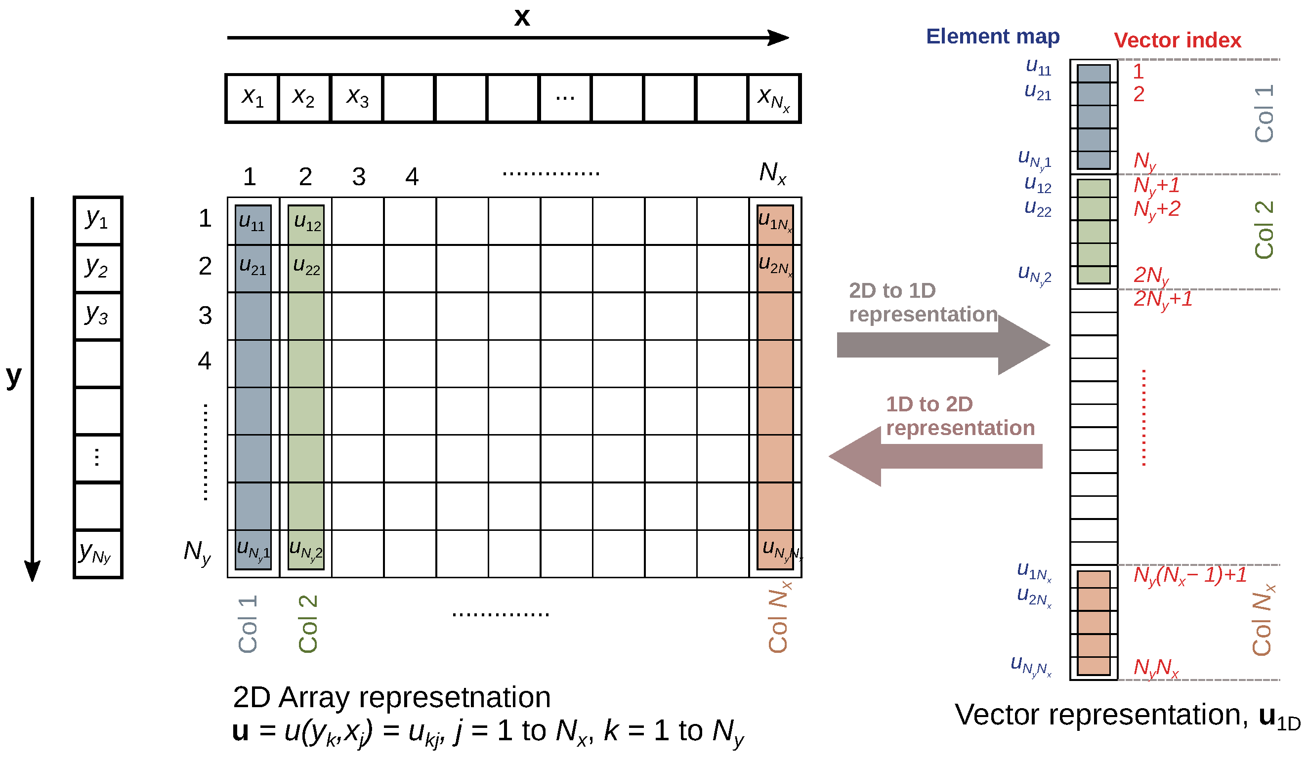
Figure 2.
Matrix first-derivative operator (with respect to y) for the two-dimensional case. has the same form as which is defined in Equation (13).
Figure 2.
Matrix first-derivative operator (with respect to y) for the two-dimensional case. has the same form as which is defined in Equation (13).

Figure 3.
Matrix first-derivative operator (with respect to x) for the two-dimensional case. refers to the element from row j and column k of the matrix defined in Equation (13).
Figure 3.
Matrix first-derivative operator (with respect to x) for the two-dimensional case. refers to the element from row j and column k of the matrix defined in Equation (13).

Figure 4.
Solution domain for the two-dimensional parallel plate capacitor problem. The boundaries defined by the red points are Neumann boundaries. The gray regions indicate the parallel plates, where Dirichlet boundary conditions are set. The light green regions have no boundary conditions enforced on them.

Figure 5.
Solution of the Poisson equation for a parallel plate capacitor: (a) potential distribution, u, and (b) electric field distribution. The colors in (b) represent the magnitude of the electric field, , and the arrow lines are electric field lines showing the direction of .
Figure 5.
Solution of the Poisson equation for a parallel plate capacitor: (a) potential distribution, u, and (b) electric field distribution. The colors in (b) represent the magnitude of the electric field, , and the arrow lines are electric field lines showing the direction of .

Figure 6.
(a) Solution domain for the two-dimensional p–n junction problem. The red points are Neumann boundaries. The gray regions indicate the inner Dirichlet boundaries. (b) The source function .
Figure 6.
(a) Solution domain for the two-dimensional p–n junction problem. The red points are Neumann boundaries. The gray regions indicate the inner Dirichlet boundaries. (b) The source function .

Figure 7.
Solution of the Poisson equation for a simplified p–n junction: (a) potential distribution, u, and (b) electric field distribution. The colors in (b) represent the magnitude of the electric field, , and the arrow lines are electric field lines showing the direction of .
Figure 7.
Solution of the Poisson equation for a simplified p–n junction: (a) potential distribution, u, and (b) electric field distribution. The colors in (b) represent the magnitude of the electric field, , and the arrow lines are electric field lines showing the direction of .

Figure 8.
(a) Solution domain for the two-dimensional arbitrary problem with external-image-defined geometry. (b) The boundary regions identified by the code. Different colors represent different boundary conditions to be enforced.
Figure 8.
(a) Solution domain for the two-dimensional arbitrary problem with external-image-defined geometry. (b) The boundary regions identified by the code. Different colors represent different boundary conditions to be enforced.

Figure 9.
Solution of the Poisson equation for an arbitrary image-defined geometry: (a) potential distribution, u, and (b) electric field distribution. The colors in (b) represent the magnitude of the electric field, , and the arrow lines are electric field lines showing the direction of .
Figure 9.
Solution of the Poisson equation for an arbitrary image-defined geometry: (a) potential distribution, u, and (b) electric field distribution. The colors in (b) represent the magnitude of the electric field, , and the arrow lines are electric field lines showing the direction of .

Publisher’s Note: MDPI stays neutral with regard to jurisdictional claims in published maps and institutional affiliations. |
© 2022 by the author. Licensee MDPI, Basel, Switzerland. This article is an open access article distributed under the terms and conditions of the Creative Commons Attribution (CC BY) license (https://creativecommons.org/licenses/by/4.0/).
Share and Cite
MDPI and ACS Style
Zaman, M.A. Numerical Solution of the Poisson Equation Using Finite Difference Matrix Operators. Electronics 2022, 11, 2365. https://doi.org/10.3390/electronics11152365
AMA Style
Zaman MA. Numerical Solution of the Poisson Equation Using Finite Difference Matrix Operators. Electronics. 2022; 11(15):2365. https://doi.org/10.3390/electronics11152365
Chicago/Turabian StyleZaman, Mohammad Asif. 2022. "Numerical Solution of the Poisson Equation Using Finite Difference Matrix Operators" Electronics 11, no. 15: 2365. https://doi.org/10.3390/electronics11152365
Note that from the first issue of 2016, this journal uses article numbers instead of page numbers. See further details here.