Abstract
A hierarchical random graph (HRG) model combined with a maximum likelihood approach and a Markov Chain Monte Carlo algorithm can not only be used to quantitatively describe the hierarchical organization of many real networks, but also can predict missing connections in partly known networks with high accuracy. However, the computational cost is very large when hierarchical random graphs are sampled by the Markov Chain Monte Carlo algorithm (MCMC), so that the hierarchical random graphs, which can describe the characteristics of network structure, cannot be found in a reasonable time range. This seriously limits the practicability of the model. In order to overcome this defect, an improved MCMC algorithm called two-state transitions MCMC (TST-MCMC) for efficiently sampling hierarchical random graphs is proposed in this paper. On the Markov chain composed of all possible hierarchical random graphs, TST-MCMC can generate two candidate state variables during state transition and introduce a competition mechanism to filter out the worse of the two candidate state variables. In addition, the detailed balance of Markov chain can be ensured by using Metropolis–Hastings rule. By using this method, not only can the convergence speed of Markov chain be improved, but the convergence interval of Markov chain can be narrowed as well. Three example networks are employed to verify the performance of the proposed algorithm. Experimental results show that our algorithm is more feasible and more effective than the compared schemes.
1. Introduction
Complex networks generally have many characteristics, such as small-world effect [1], scale-free property [2], community structure [3], etc. Since the concept of community [3] was put forward in 2002, there has been an upsurge in the study of community structure in academic circles. The significance of studying community structure is that it is helpful to understand the function of a complex network, find the hidden rules in a complex network, and predict the connection of missing links. Many solutions have been proposed to solve the problem of how to partition a complex network. Some of them use the graph segmentation method [4,5]. Their work focuses on dividing the network of the number of communities and the number of members in the community in advance. However, this solution is not rigorous. The purpose of community detection is to find the natural division of networks, and there is no limit to the specified number. Although the method based on partition–optimization [6,7] does not need to know the number of members in the community in advance, it still needs to specify the number of communities in advance. In order to solve this problem, some detection methods are based on label propagation [8,9]. This kind of method not only does not need prior conditions, but also has the characteristics of low time complexity and fast calculation speed. However, the research direction for these kinds of methods is in how to improve the accuracy and stability of the results of community division.
As the research has matured, it has been found that some real networks, such as metabolic networks [10] and brain neural networks [11], have obvious hierarchical structures [12,13,14]. The hierarchical structure can not only reflect the community structure, but also reveal the hierarchical organizational relationship among the members of the community. In the early days, some methods based on divisive hierarchical clustering were proposed [10,15]. Although this kind of method can accurately identify the community structure, it cannot identify the number of communities, and its high computational cost and time complexity make it unsuitable for large-scale networks. In order to solve this problem, modularity function base solutions were proposed to mine community structure [16,17]. Its core is to use a modular function Q to quantify the strengths and weaknesses of the community structures. Although these solutions have greatly enriched the scale of the network and can accurately discover the number of communities, the relationships among members of communities have not been well discovered. Moreover, it is not clear whether the generated hierarchy reflects the real structures of the networks or is only a product of the algorithm itself. In addition, the basic assumption of the modularity is that there is no community structure in random networks, which is questioned by several studies [18,19]. At the same time, the modular function Q has other disadvantages, such as resolution limit [20] and extreme degeneracies [21]. Thus, designing a model that can truly reflect the network structure is an important and urgent task.
In recent years, some scholars have put forward the concept of hierarchical random graph models [22,23], as shown in Figure 1. It is also a dendrogram in nature. The maximum likelihood method [24] and Markov Chain Monte Carlo [25,26] method are applied to the model to sample all possible dendrograms, so as to realize the fitting of hierarchical model and observation network data. Different from other clustering algorithms that can only generate a single hierarchical structure, this method can generate a set of dendrograms, and each of them is reasonable. However, with the growth of the size of networks, the time cost of using MCMC algorithm to find dendrogram models that can reflect the observed data is very large. Therefore, it is urgent to find a solution that can not only reduce the time cost but also accurately reflect the real structure of a network.
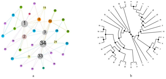
Figure 1.
A real network and its corresponding hierarchical random graphs. (a) A network visualization, in which the real name of each vertex is hidden as a number. (b) A possible hierarchical random graph model, in which the leaf nodes correspond to the vertices of the real network, and the color depth of each non-leaf node represents the connection possibility between the leaf nodes.
Inspired by some extended MCMC algorithms [27,28,29,30], a new algorithm called TST-MCMC based on MCMC algorithm is proposed in this paper. The new algorithm introduces the mechanism of two-state transition (TST), that is, two candidate states that are randomly generated in the process of an iteration. In order to prevent the generation of multiple Markov chains under this mechanism, we introduce a competition mechanism to keep the worse of the two candidate states from being accepted. Compared with MH-MCMC algorithm [26], the proposed algorithm can not only improve the convergence speed, but also improve the quality of hierarchical random graphs obtained during convergence. The contributions of this paper are as follows:
- (1)
- A novel algorithm for sampling hierarchical random graphs is proposed. The algorithm allows two candidate states to be generated and takes the one with the maximum likelihood in the Markov process to speed up the traversal of hierarchical random graph sets.
- (2)
- By means of competition, eliminate the worse of the two candidate states to avoid producing multiple Markov chains. At the same time, this method indirectly leads to the Markov chain with more detailed balance.
The rest of this paper is organized as follows. Section 2 introduces the related work based on hierarchical random graph model. Section 3 introduces the details and design objectives of the proposed TST-MCMC algorithm. At the same time, in this section, we use an example to show how our algorithm works. Section 4 analyzes the performance of our method through four groups of experiments. Finally, we conclude this paper in Section 5.
2. Related Work
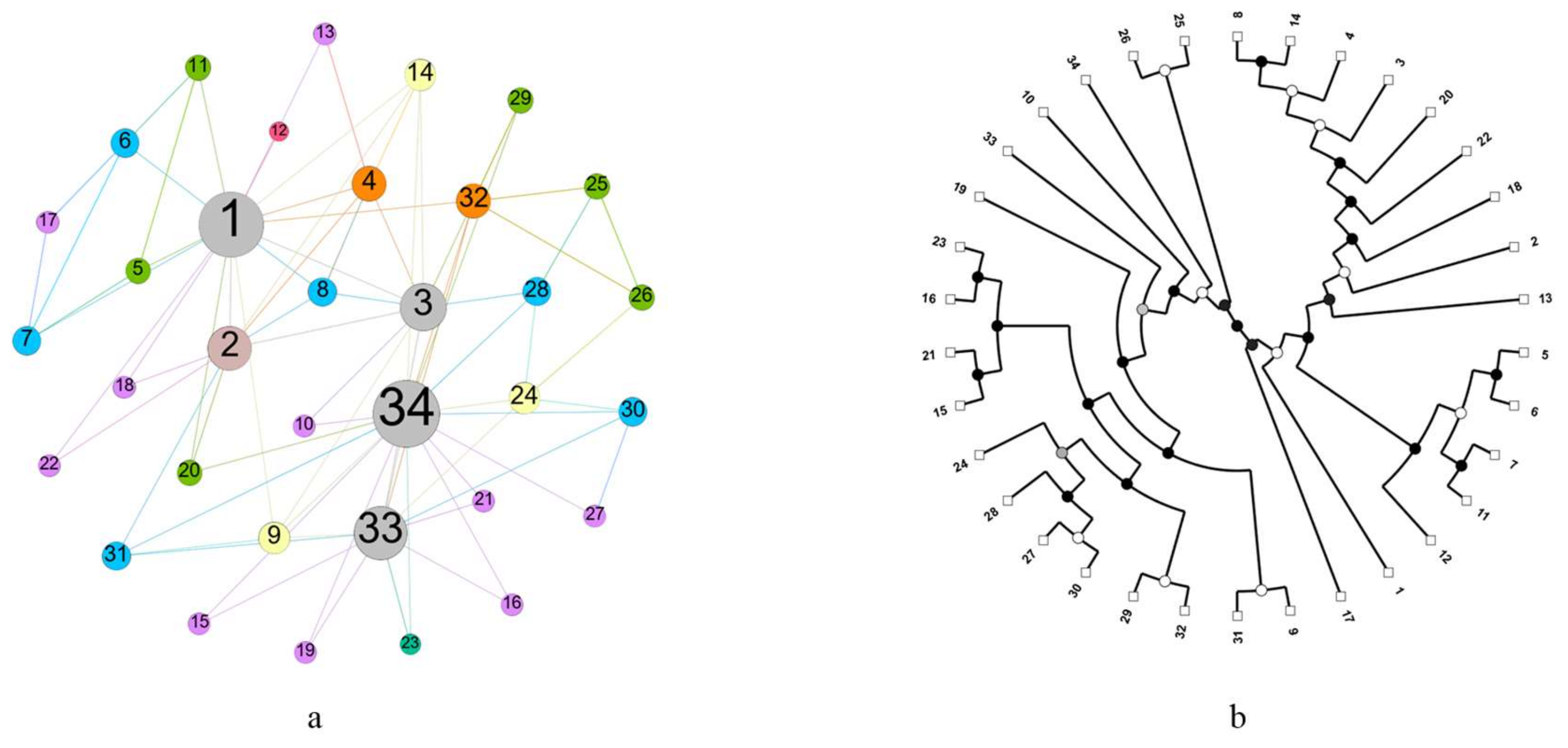
In 2007, Clauset et al. [22] first proposed the concept of the hierarchical random graph model. Let the real network be a simple undirected graph with n vertices. Figure 2a shows an example of a small network with 7 vertices. A hierarchical random graph can be regarded as a dendrogram (essentially a binary tree), which is composed of internal nodes, internal edges, and leaf nodes, as shown in Figure 2b. The leaf nodes correspond to the vertices in graph . An internal edge connects two internal nodes, and each internal node has a probability , whose calculation formula is Equation (1).
where and represent the numbers of leaf nodes of left and right subtree rooted at an internal node , respectively. represents the numbers of connected edges in the graph whose endpoints have the internal node as their lowest common ancestor in . Figure 2b shows the value of of each internal node calculated by Equation (1).
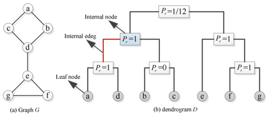
Figure 2.
A sample network and hierarchical random graph composition. (a) A small sample network with seven vertices. (b) The structure of the hierarchical random graph.
To what degree the dendrogram reflects the true structure of the network can be determined by the likelihood function, as shown in Equation (2).
where the larger the likelihood is, the better the dendrogram fits with the real network [23]. However, it is difficult to maximize the resulting likelihood function analytically over the space of all dendrograms. Fortunately, this problem can be solved by using a Markov Chain Monte Carlo (MCMC)-based algorithm called the Metropolis–Hastings algorithm (MH-MCMC) [26]. In order to ensure the convergence of MCMC algorithm, the Metropolis–Hastings (M–H) [25,31] rule is used to accept or reject the dendrogram generated by MCMC algorithm.
At first, the HRG model is proposed for those networks with single node type, single edge type, and obvious hierarchical structure. Some algorithms for searching community structure are also designed for this single entity network [17,32]. Unfortunately, in real networks, the type of nodes and the edge relationships are not single, just like a binary network, which is the simplest heterogeneous network. A bipartite network consists of two types of nodes, that is, there are no edges between the same types of nodes, and there are edges between different types of nodes. There are a large number of bipartite networks in the real world, such as the scientific paper collaboration network, the film actor network, the audience song network, etc. Therefore, the bipartite network is also an important object in complex network research. In 2011, Chua et al. [33] proposed the BHRG model to adapt to binary networks. By using theoretical derivation and experimental comparison, they prove in detail that the BHRG model can give higher likelihood than the HRG model in bipartite networks. In other words, for the same dendrogram , the likelihood calculated by BHRG model is not less than that calculated by HRG model. In the same year, Allen et al. [34] proposed a weighted hierarchical random graph (wHRG) model for weighted networks and also proposed a vectorized hierarchical random graph (vHRG) model for weighted networks with multiple attributes on the edges.
In recent years, much important work has been carried out on the applications of the HRG model. In 2009, Wu et al. [35] conducted an exploratory analysis of protein translation regulatory networks using hierarchical random graphs. In 2012, Fountain et al. [36] used hierarchical random graphs to classify words in a text. In 2015, Yang et al. [37] used hierarchical random graphs to predict brain network links. In 2018, Gao et al. [38] proposed a uniform framework based on hierarchical random graph models to generate a perturbed social network under the group-based local differential-privacy criteria. Thus, the system constructed by the HRG model is becoming more and more perfect. This expands the applicability of the HRG model. However, due to the time complexity of MCMC algorithm, the HRG model and its variants are only suitable for dealing with small networks with fewer than several thousand nodes, which greatly reduces its practicability. Therefore, improvement of computational performance to allow for larger networks is also one of the directions worth exploring.
3. TST-MCMC Algorithm
The theoretical convergence speed of MH-MCMC algorithm in small-scale networks is optimistic. A network with thousands of vertices is practiced in the paper [22], and the mixing speed of MH-MCMC algorithm is relatively fast. However, with the linear growth of the number of vertices, the number of hierarchical random graphs increases exponentially. The number of dendrograms with n leaves is super-exponential, growing like Equation (3).
where the operator “!!” denotes double factorial. This will cause several problems: (1) it takes a great deal of time to traverse all possible dendrograms on a Markov chain. MH-MCMC algorithm may need exponential time [39] to converge in the worst case. (2) In the later stage of the MCMC operation, the convergence rate slows down gradually. The optimal hierarchical random graph obtained with this local convergence does not fit well with the observed data. Although better results can be achieved by prolonging the sampling time or experimenting with multiple experiments, the time cost is enormous. Due to these problems, we propose a two-state transition MCMC (TST-MCMC) algorithm to efficiently search local ideal hierarchical random graphs.
3.1. Subtree Rearrangement
Before introducing the TST-MCMC algorithm, it is necessary to introduce how to select a set of transformations between possible dendrograms in the process of creating a Markov chain. We use a method called “subtree rearrangement” to transform a given dendrogram into another. By randomly selecting an inner edge, the inner edge connects the head node and the tail node and records an attribute called “type”. There are two types of inner edges: the left type or the right type. The inner edge of type “left” is on the left side of its head node, and the inner edge of type “right” is on the right side of its head node. We specify that the head node of an inner edge is the parent of its tail node. The detailed process of subtree rearrangement is as follows:
- 1.
- The type of inner edge is “left”
- transformation
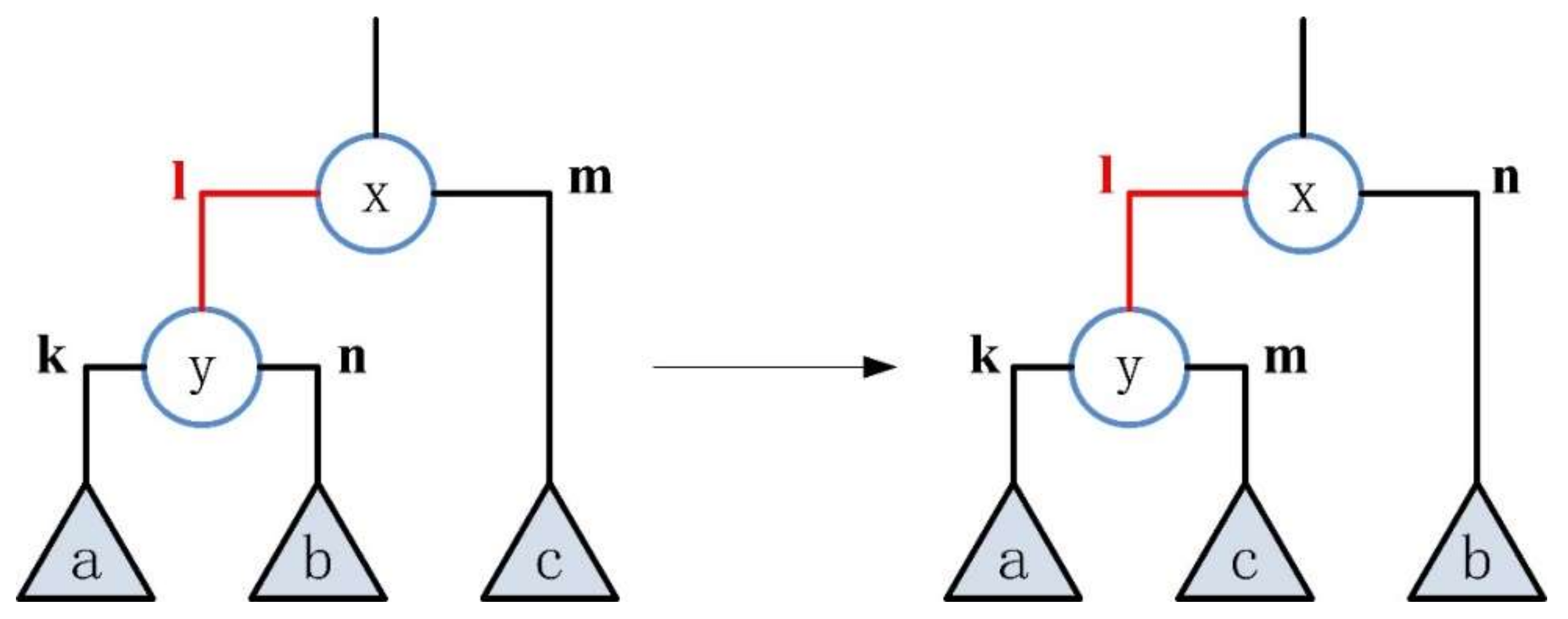
Randomly select an inner edge of type “left” and perform an transformation on it, as shown in Figure 3. Let be a randomly selected internal edge, and its head node is and its tail node is . According to the above provisions, it can be clearly judged that the type of this edge is “left”. Here, and respectively represent the left and right subtrees of the tail node , and represents the right subtree of the head node . This situation can be described as . In this case, the goal of rotation is to change to , that is, to swap the position of edge and , and the position of subtree also swap.

Figure 3.
The transformation of the inner edge of type “left”.
- transformation
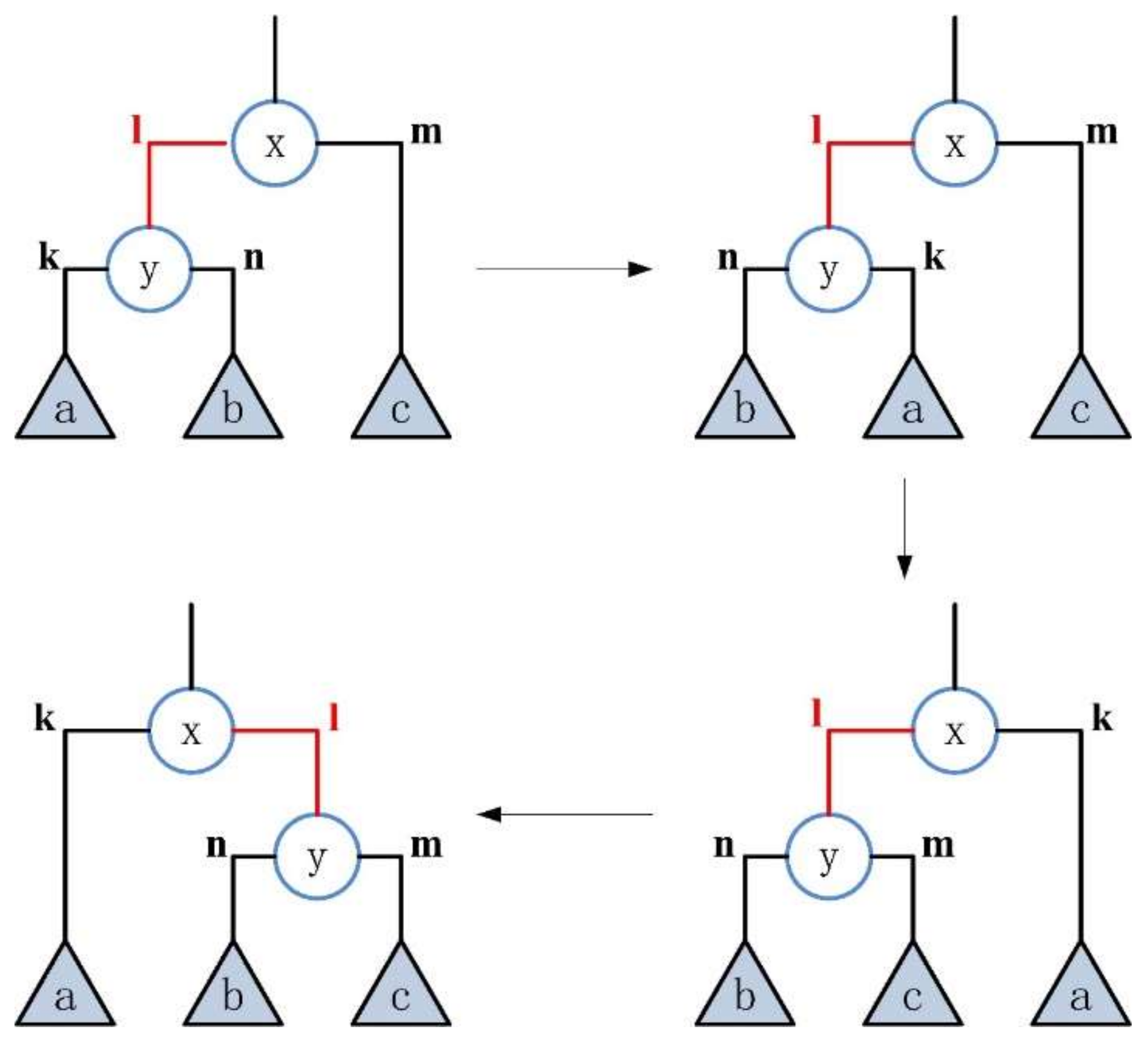
Randomly select an inner edge of type “left” and perform a transformation on it, as shown in Figure 4. The state before the transformation is the same as that before the transformation, ie , and the target of transform is →. The specific steps are: (1) exchange the positions of edge and subtree with edge and subtree ; (2) exchange the positions of edge and subtree with edge and subtree a; (3) exchange the positions of the inner edge and the subtree connected with it with edge and subtree .

Figure 4.
The transformation of the inner edge of type “left”.
- 2.
- The type of inner edge is “right”
- transformation
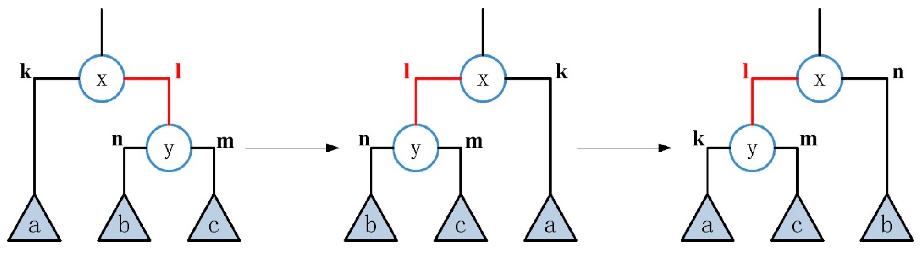
Randomly select an inner edge of type “right” and perform an transformation on it, as shown in Figure 5. Let be a randomly selected internal edge, and its head node is and its tail node is . Here, and respectively represent the left and right subtrees of the tail node , and a represents the right subtree of the head node . The current state can be represented by . Here, the goal of transformation is to convert the state to . The specific steps are: (1) exchange the position of edge and subtree a with the inner edge and the subtree connected with it; (2) exchange the positions of edge and subtree with edge and subtree .
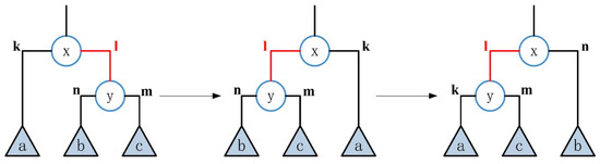
Figure 5.
The transformation of the inner edge of type.
- transformation
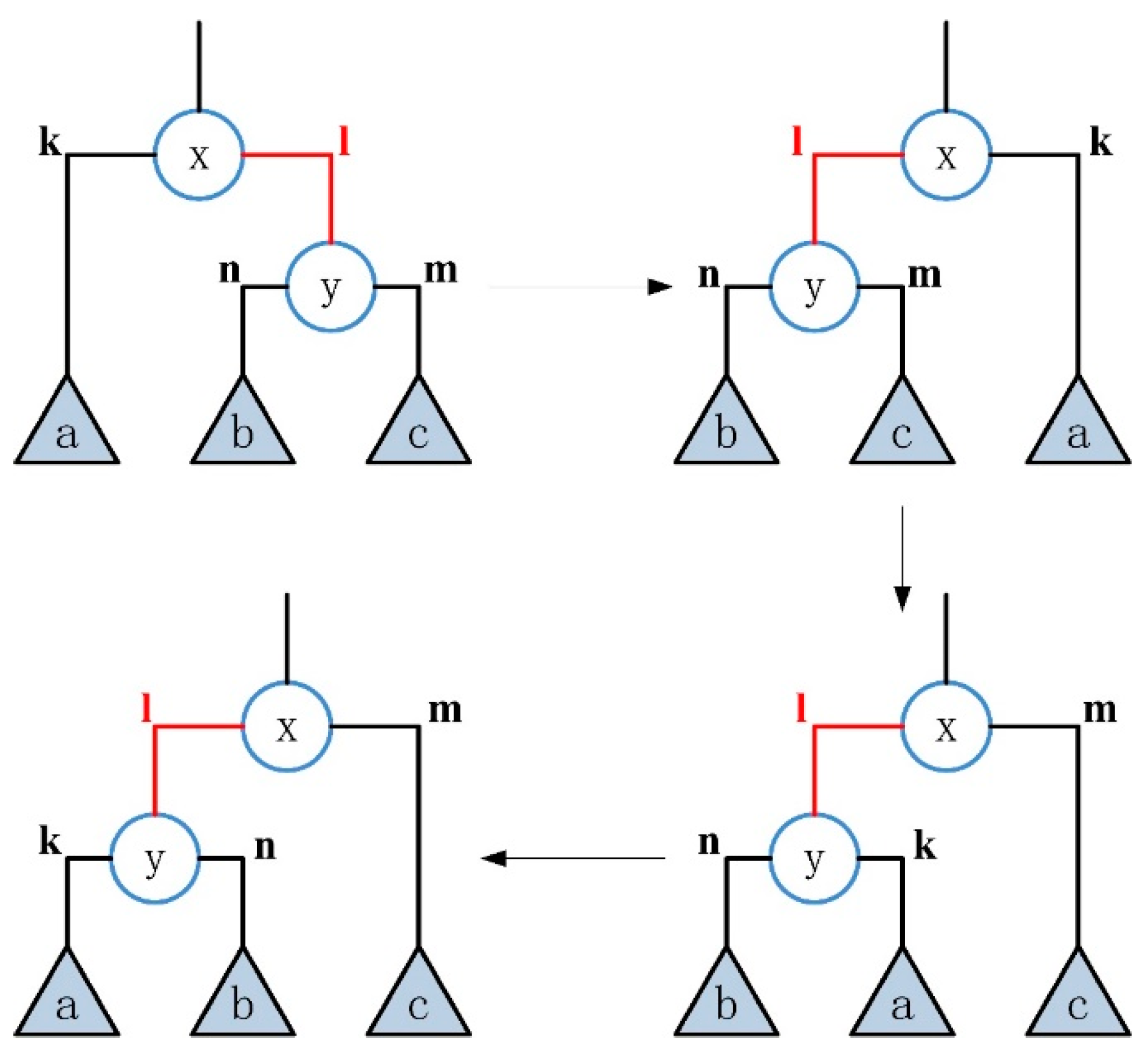
Randomly select an inner edge of type “right” and perform a transformation on it, as shown in Figure 6. The state before the transformation is the same as that before the α transformation, that is, the aim of transformation is to transform the state to . The specific steps are: (1) exchange the position of the inner edge and the subtree connected with it with the edge and the subtree ; (2) exchange the positions of edge and subtree with edge and subtree ; (3) exchange the positions of edge and subtree with edge and subtree .
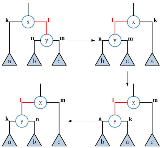
Figure 6.
The β transformation of the inner edge of type.
The above transformation process is reversible. If only the initial state and result state of the tree graph are retained, it can be found that there are only three kinds of subtree arrangement order, which are , , . In other words, any one of them can be transformed into the other two states. Figure 7 shows the relationship between the three states. The scheme of subtree rearrangement can theoretically traverse all situations.
Figure 7.
Subtree rearrangement, starting from any one state, can be converted into the other two states.
3.2. TST-MCMC Algorithm
Suppose the state of the hierarchical random graph at time is . The Markov chain specifies that the hierarchical random graph state at the moment of is only related to . TST-MCMC algorithm does not really produce two Markov chains, but always produces two temporary states at the time of . There is no correlation between and , but both are related to the state . This accords with the property of Markov chain. The better one is always left between and as the real state at time .
The specific operation is as follows: two different inner edges , are randomly selected from inner edges at one time, and the selected inner edges , are far apart in the dendrogram ; then, randomly rearrange the selected internal edges, respectively.
Using the above method, two new dendrograms are obtained. We calculate the likelihood for the and compare them, keep one with higher likelihood, and then use the M–H rule to accept or reject the dendrogram. Specific steps are shown in Algorithm 1.
3.3. Performance Analysis
The MH-MCMC algorithm produces only one kind of dendrogram per iteration, while TST-MCMC algorithm can produce two different dendrograms per iteration. Assuming that the dendrogram generated each time is not repeated with the past, under the same number of iterations, the likelihood generated by TST-MCMC algorithm is greater than or equal to that generated by MH-MCMC algorithm. Therefore, in non-extreme cases, TST-MCMC algorithm can converge to equilibrium with fewer iterations than MH-MCMC algorithm. Another advantage of this method is that the convergence is more stable. Suppose that time is in convergence equilibrium and the dendrogram state is , then the dendrogram state obtained by MH-MCMC algorithm at is , and the dendrogram obtained by the improved algorithm is . If is better than , keep , otherwise keep . Obviously, even in the most extreme cases, the convergence stability of this algorithm is only the same as MH-MCMC algorithm, but in general, this method is much more stable than MH-MCMC algorithm.
| Algorithm 1 TST-MCMC |
| Let be the observed Graph. Build the initial HRG Compute likelihood of While (true) ←Randomly select two different internal nodes(non-root) Transform the dendrogram according to Compute likelihood of according to Equation (2) Transform the dendrogram according to Compute likelihood of according to Equation (2) ≥ 0 then Randomly generate a value ∈[0,1] then Record the current dendrogram structure else Keep intact else Randomly generate value ∈[0,1] then Record the current dendrogram structure else Keep intact |
3.4. Example
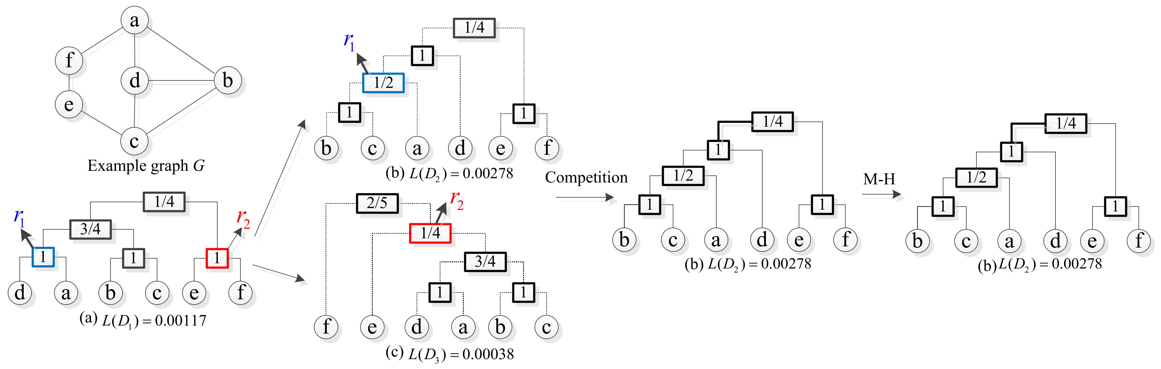
Assuming that the current state of the Markov chain is shown in Figure 8a. Under this state, two internal nodes , are randomly selected, in which the of equal 1 and of equal 1 according to Equation (1). Then, let the two internal nodes perform a subtree rearrangement respectively, in which the selected internal node is rearranged into (shown in Figure 8b), and the selected internal node is rearranged into (shown in Figure 8c). The likelihoods of the two dendrograms are calculated according to Equation (2):
Figure 8.
An example of the process of TST-MCMC algorithm. (a) Dendrogram of current state. (b) Dendrogram transformed by . (c) Dendrogram transformed by .
Then, keep the dendrogram with high likelihood probability. Here, we keep , and according to M-H stardard, ≥ 0, hence accept →. Then, loop the above process again, and so on.
If using MH-MCMC algorithm, one internal node is selected at each conversion. Suppose the internal node is selected for the first time. After transformation, →. According to the M-H standard, keep the state of 1. Then, the internal node is selected for the second time, and after conversion, →. According to the M-H standard, is accepted as the current state. The MH-MCMC algorithm takes two rounds of iteration to get the same result as TST-MCMC algorithm, which shows that TST-MCMC algorithm is better than MH-MCMC algorithm in the number of iterations required for convergence. The following experiments show that the time efficiency of TST-MCMC algorithm is better than MH-MCMC algorithm.
4. Experiments and Analysis
4.1. Experimental Setup
In order to verify the performance of the proposed TST-MCMC algorithm, three different real network datasets, which are illustrated in Table 1, were employed to compare with the MCMC sampling algorithm. The purposes of our experiments were (1) to determine whether the proposed TST-MCMC can converge faster than the MCMC, and (2) to determine, under the condition that both algorithms tend to be balanced, which method can give a better structure.

Table 1.
Datasets.
The Zachary Karate Club network [40] consists of 34 nodes and 72 edges, in which each node represents a member of the club, and each edge represents the friendship between two members of the club. The network is an undirected and unweighted network.
The Metabolic network [41] consists of 453 nodes and 2025 edges. Each node in the network represents metabolites (such as proteins), and each edge represents the interaction between two metabolites. In the network, some edges are loops because certain metabolites can iterate on themselves, and we removed these self-cycling edges during the experiments; thus, the network is an undirected powerless network.
The Yeast network [42] contains 2375 nodes and 11,693 edges, in which each node represents the type of protein, and each edge represents the interaction between two proteins. It is an undirected and powerless network.
All the experiments were conducted on a platform with the Deepin V15.11 operating system based on the Linux kernel developed by Wuhan Deepin Technology Co., Ltd. (located at Wuhan, China), which is equipped with Samsung 4 GB memory and an Intel Core i3-2100 CPU.
4.2. Experimental Analysis
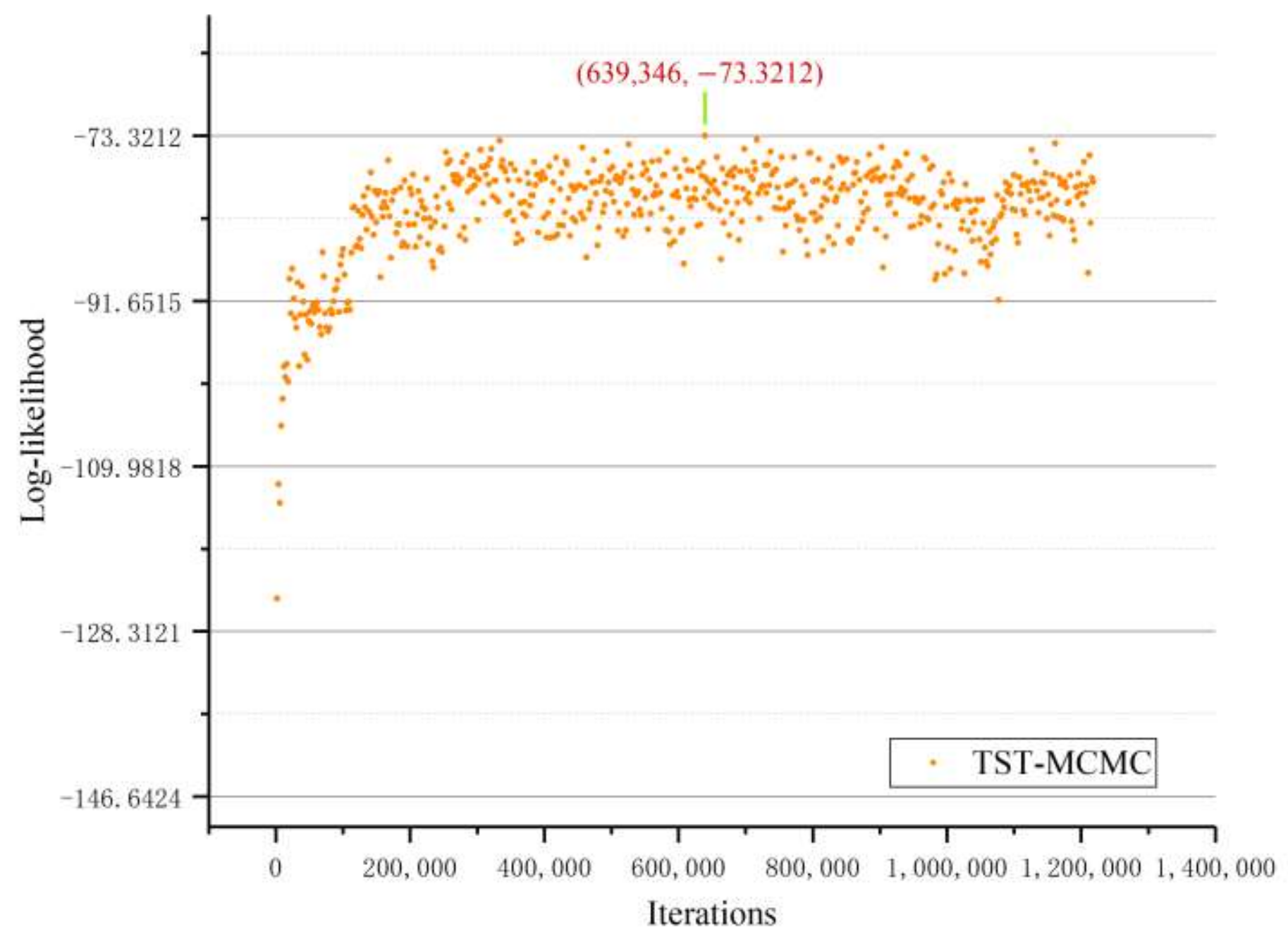
First, the Zachary Karate Club network was chosen to verify the correctness of the proposed TST-MCMC method, i.e., that it can reach the best likelihood value. The likelihood value was recorded every 2049 steps, as shown in Figure 9. When the proposed TST-MCMC algorithm moved 639,346 times, it found the best likelihood value = −73.32, which was given by Clauset et al. [22].

Figure 9.
Relationship between the log-likelihood and the number of MCMC iterations.
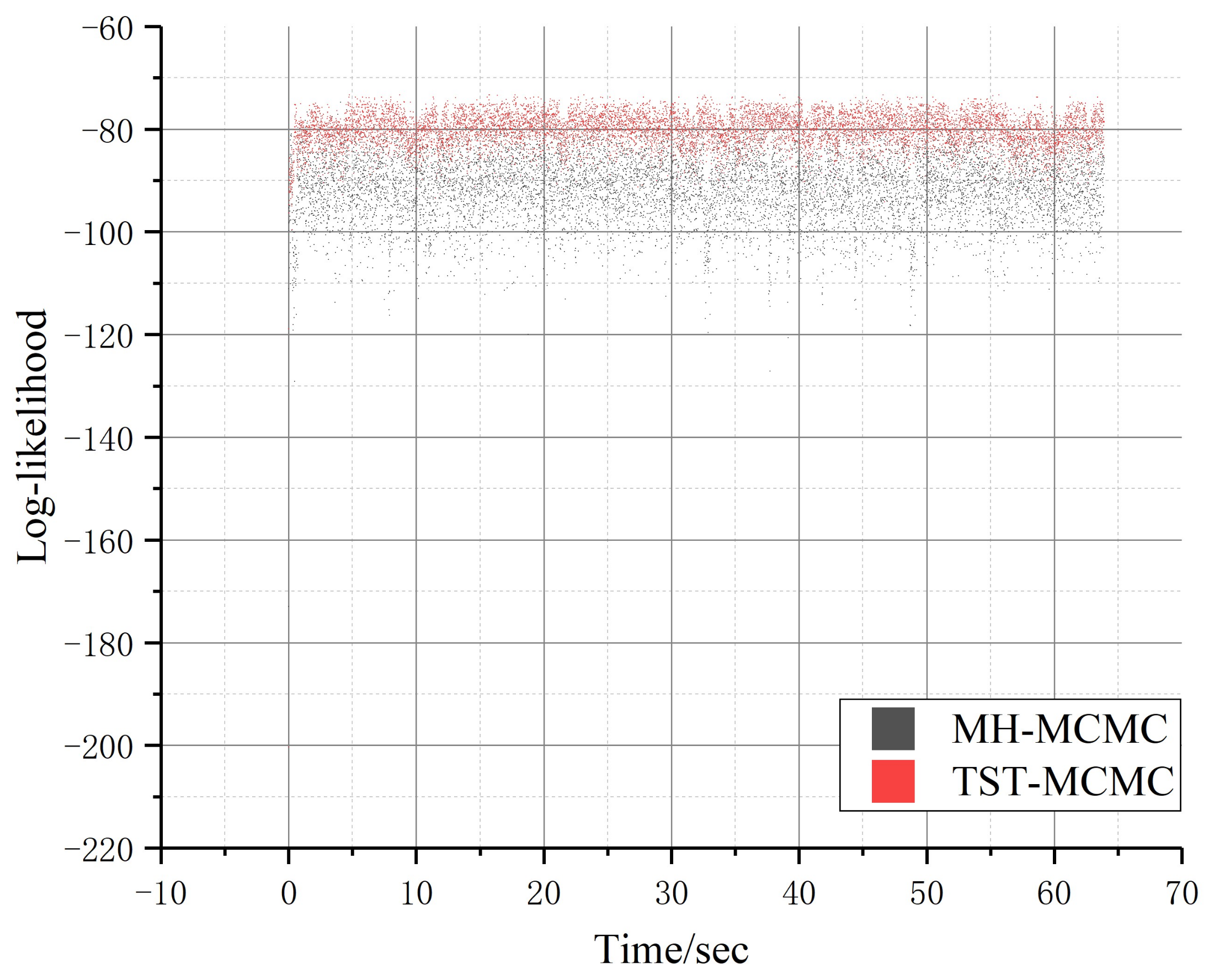
Secondly, we compared the proposed TST-MCMC method with MH-MCMC algorithm on the Zachary Karate Club network. Since the Zachary Karate Club has only 34 nodes and 72 edges, we limit the experimental running time to 1 min. The experimental results are shown in Figure 10 and Figure 11. As can be seen from Figure 10, both the proposed algorithm and MH-MCMC algorithm can quickly converge to equilibrium in small-scale networks. However, the proposed algorithm has a narrower convergence interval than MH-MCMC algorithm, and when the convergence is balanced, the local likelihood maximum obtained by the proposed algorithm is higher than that of MH-MCMC algorithm in the same time.

Figure 10.
Comparison of two algorithms in Zachary Karate Club network (relationship between log-likelihood and iterations, in which the red scatter represents TST-MCMC algorithm and the black scatter represents MH-MCMC algorithm).
Figure 11.
The comparison of the total number of iterations between the two algorithms and the number of iterations corresponding to finding the optimal solution.
Figure 11 shows the comparison of iterations of the two algorithms within 1 min and the corresponding comparison of iterations when the local best likelihood value is found. In 1 min, the total number of iterations obtained by using the proposed algorithm is about half that of MH-MCMC algorithm. This is because the proposed algorithm randomly selects two edges for state transition at the beginning and finally retains the better result, while MH-MCMC algorithm randomly selects one edge for state transition at a time. Therefore, the proposed algorithm will sacrifice some extra computing time. Although MH-MCMC algorithm is about twice as fast as the proposed algorithm in terms of iteration speed, it can be found that the proposed algorithm only uses one-fourteenth of MH-MCMC algorithm by comparing the corresponding iteration times when the two algorithms find the local best likelihood value. In conclusion, the proposed algorithm is seven times faster than MH-MCMC algorithm in finding the local best likelihood value. Therefore, sacrificing a little extra computation is well worth it.
In order to further verify the performance of the proposed TST-MCMC method, we conducted experiments on the Metabolic network with 453 nodes and 2025 edges. Figure 12 shows the convergence of the two algorithms within one hour.
Figure 12.
Comparison of two algorithms in metabolic network (the function of the likelihood logarithm with running time; the red one represents TST-MCMC algorithm, while the black one represents MH-MCMC algorithm).
As can be seen from Figure 12, the fluctuation range of the likelihood in the equilibrium state of TST-MCMC algorithm is more stable than the fluctuation range of the likelihood in the equilibrium state of MH-MCMC algorithm. In addition, the likelihood obtained by TST-MCMC algorithm at equilibrium is better than that of MH-MCMC algorithm. Notably, the polyline graph for TST-MCMC algorithm shows a jitter in about 2 min. This is because the state after the Markov chain state transition is not ideal, and there will be a short bottleneck period during this period. We recorded the best likelihood that the two algorithms can find within a limited time. The best likelihood value L (calculated by Equation (2)) of MH-MCMC algorithm is −4415.6, while the likelihood value L (calculated by Equation (2)) of the improved algorithm is −4252.9. The convergence result of TST-MCMC algorithm is improved by 3.6% compared with MH-MCMC algorithm in a single experiment.
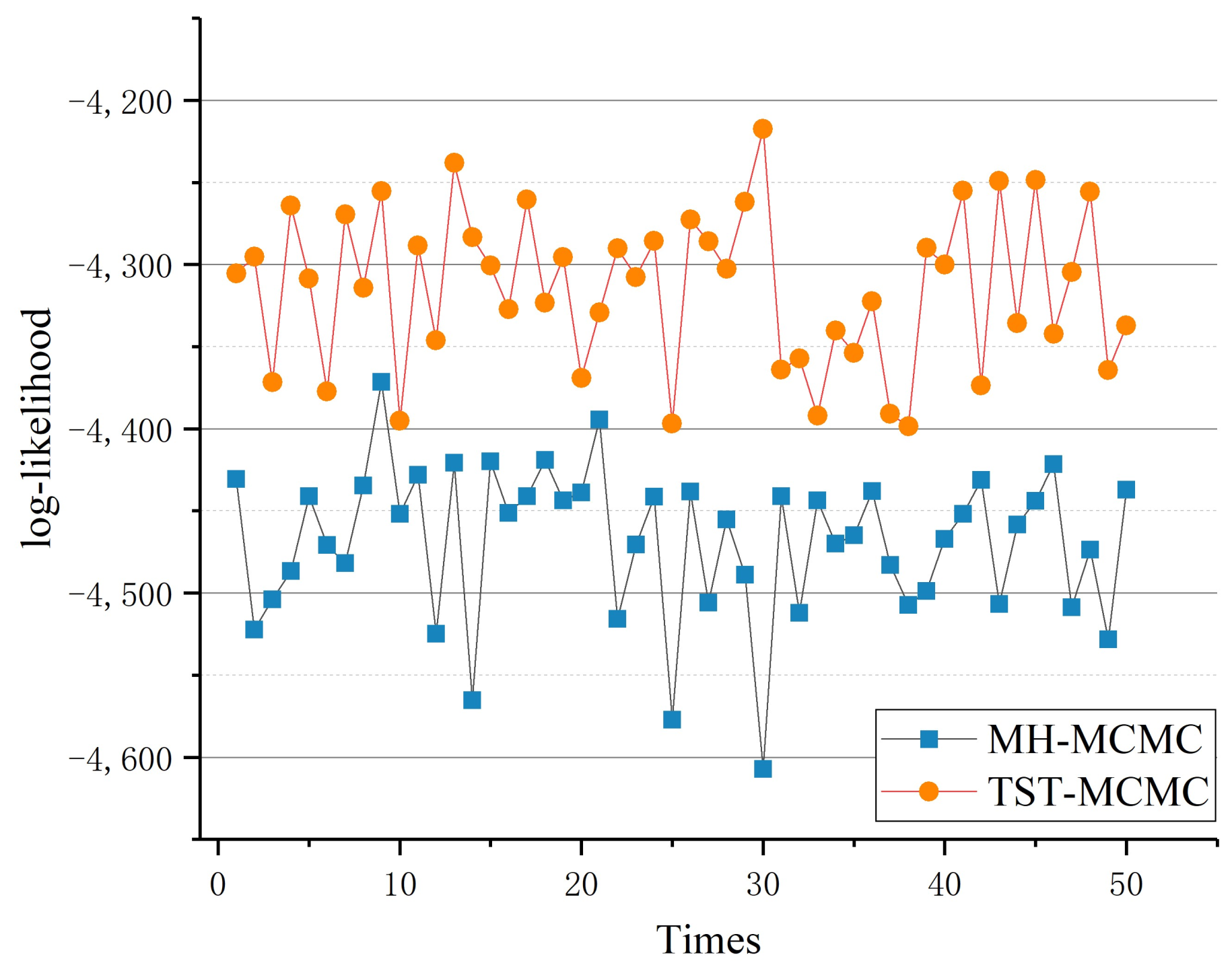
Furthermore, we conducted 50 experiments with the Metabolic network and recorded the best likelihood values that can be found by the two algorithms in each experiment. The duration of each time of experiments lasted 1 h. The experimental results are shown in Figure 13.
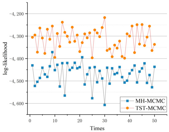
Figure 13.
Comparison of 50 sample experiments.
It can be seen that in most cases, the new algorithm finds a higher likelihood value, which means that the new algorithm can always find a better dendrogram. The mean value and standard deviation of the best likelihood value of 50 experimental iterations is shown in Table 2.
Table 2.
The mean value and the standard deviation of the best likelihood value of 50 experimental iterations.
As shown in Table 2, among the 50 samples, the average likelihood obtained using TST-MCMC algorithm is 154.34 higher than that of MH-MCMC algorithm. This means that the proposed algorithm can more accurately discover hierarchical random graph models that match the observed data than MH-MCMC algorithm. From the results of the standard deviation, although the likelihood standard deviation obtained by the proposed algorithm is only 1.61 larger than that of MH-MCMC algorithm, it is acceptable to sacrifice a little bit of stability in exchange for a hierarchical random graph model with a larger gap.
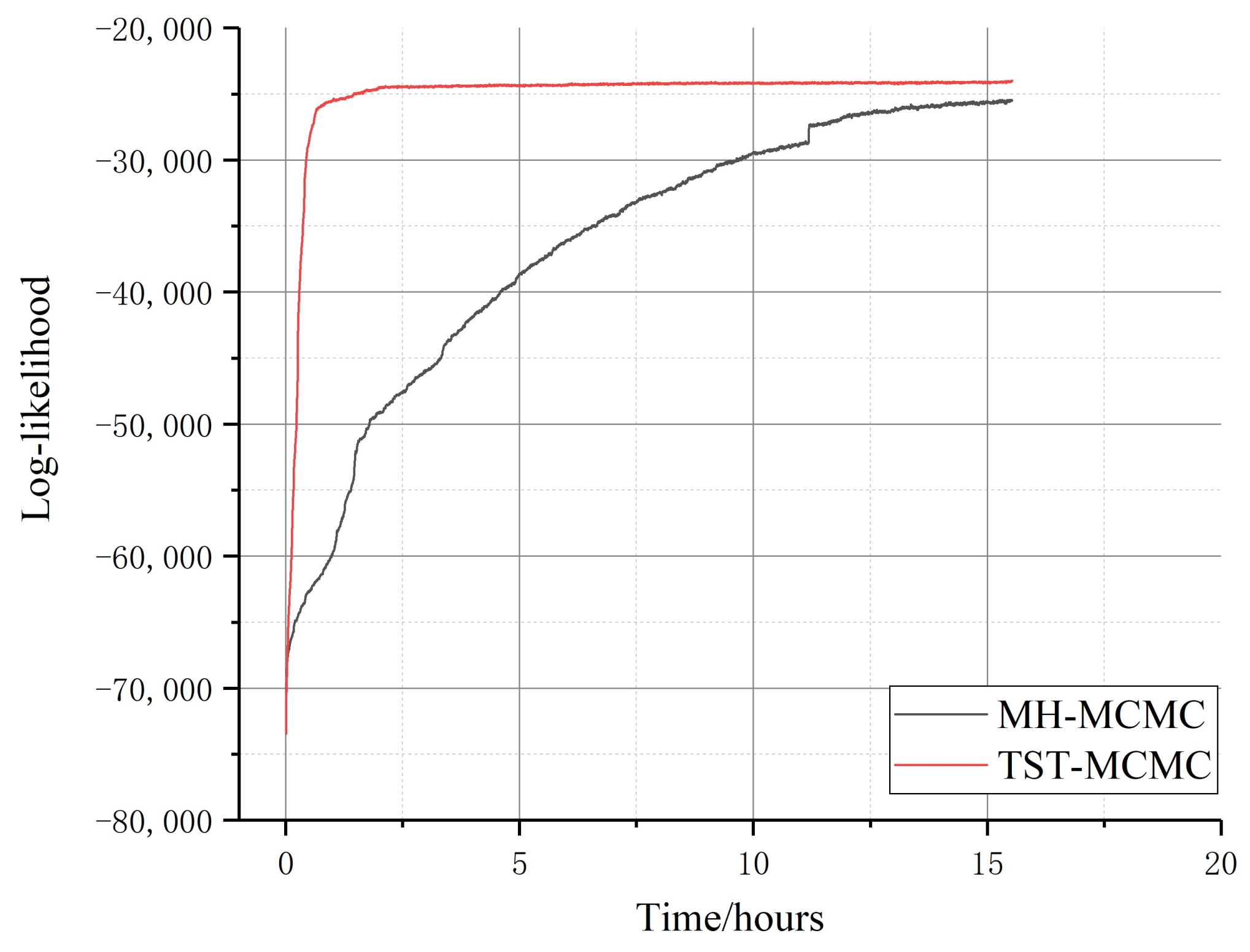
Further, we conducted the test on the Yeast network with 2375 nodes and 11,693 edges; the experimental results are shown in Figure 14.
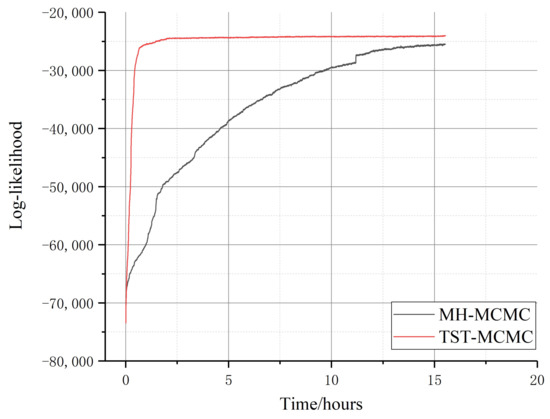
Figure 14.
Comparison of two algorithms in protein interaction network (the function of likelihood logarithm with time; red represents TST-MCMC algorithm, and black represents MH-MCMC algorithm).
It can be seen that the convergence speed of MH-MCMC algorithm is significantly slower than that of TST-MCMC algorithm on large datasets. Compared with MH-MCMC algorithm, the convergence speed of the proposed algorithm is about 83% higher. Although MH-MCMC algorithm gradually approaches equilibrium after 15 hours, its local likelihood best value is still lower than that of the proposed algorithm.
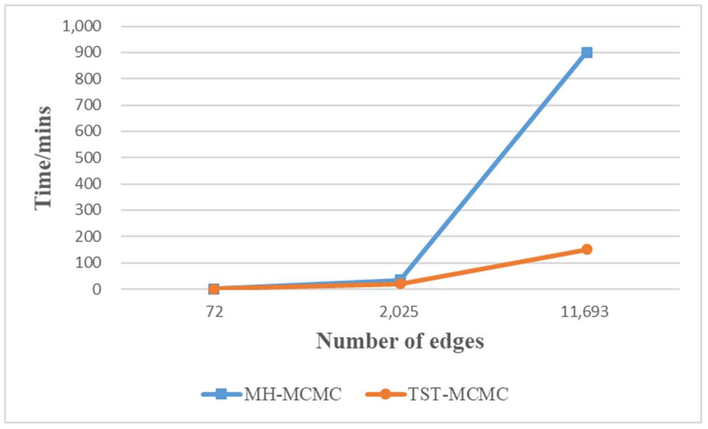
Finally, we compare the convergence speed of MH-MCMC algorithm and TST-MCMC algorithm on the three mentioned networks. As shown in Figure 15, the abscissa represents the edges of the networks, and the ordinate represents the time (in minutes) of the algorithms at equilibrium. The curves in the Figure 15 show that the larger the networks scale, the faster the convergence speed of TST-MCMC algorithm is than that of MH-MCMC algorithm. Therefore, TST-MCMC algorithm has the potential to be applied to larger scale networks.
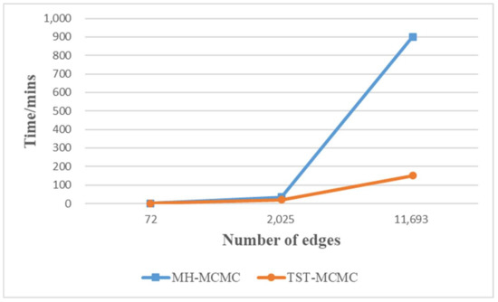
Figure 15.
For three networks of different sizes, the time spent at equilibrium between MH-MCMC algorithm and TST-MCMC algorithm.
5. Conclusions
An improved MCMC algorithm called TST-MCMC for efficiently sampling hierarchical random graphs is proposed in this paper. TST-MCMC generates two candidate state variables during a state transition and introduces a competition mechanism to filter out the worse of the two candidate state variables. The experimental results show that TST-MCMC algorithm converges faster and the fluctuation range of the likelihood value at equilibrium is smaller compared with MH-MCMC algorithm. Thus, TST-MCMC algorithm is more feasible and more effective than the compared schemes.
Author Contributions
Conceptualization, D.Z. and Z.T.; methodology, D.Z.; software, D.Z.; validation, D.Z., Z.T. and S.H.; formal analysis, D.Z. and Z.T.; investigation, D.Z.; resources, Z.T.; data curation, Z.T. and H.X.; writing—original draft preparation, D.Z.; writing—review and editing, D.Z. and Z.T.; visualization, D.Z.; supervision, Z.T.; project administration, Z.T.; funding acquisition, Z.T. All authors have read and agreed to the published version of the manuscript.
Funding
This research is partially funded by the National Natural Science Foundation of China (NSFC) (No. 61170110), Zhejiang Provincial Natural Science Foundation of China (LY13F020043), and the scientific research project of Zhejiang Provincial Department of Education (Project No. 21030074-F).
Data Availability Statement
Data is contained within the article.
Conflicts of Interest
The authors declare no conflict of interest.
References
- Watts, D.; Strogatz, S. Collective Dynamics of Small World Networks. Nature 1998, 393, 440–442. [Google Scholar] [CrossRef]
- Barabasi, A.-L.; Albert, R. Emergence of Scaling in Random Networks. Science 1999, 286, 509–512. [Google Scholar] [CrossRef] [PubMed] [Green Version]
- Girvan, M.; Newman, M. Community structure in social and biological networks. Proc. Natl. Acad. Sci. USA 2002, 99, 7821–7826. [Google Scholar] [CrossRef] [PubMed] [Green Version]
- Kernighan, B.; Lin, S. An Efficient Heuristic Procedure for Partitioning Graphs. Bell Syst. Tech. J. 1970, 49, 291. [Google Scholar] [CrossRef]
- Pothen, A.; Simon, H.; Liou, K.-P. Partitioning Sparse Matrices with Eigenvectors of Graphs. SIAM J. Matrix Anal. Appl. 1990, 11, 430–452. [Google Scholar] [CrossRef]
- Kanungo, T.; Mount, D.; Netanyahu, N.; Piatko, C.; Silverman, R.; Wu, A. A Local Search Approximation Algorithm for k-Means Clustering. Comput. Geom. 2004, 28, 89–112. [Google Scholar] [CrossRef]
- Park, H.-S.; Jun, C.-H. A simple and fast algorithm for K-medoids clustering. Expert Syst. Appl. 2009, 36, 3336–3341. [Google Scholar] [CrossRef]
- Zhang, X.-K.; Ren, J.; Song, C.; Jia, J.; Zhang, Q. Label propagation algorithm for community detection based on node importance and label influence. Phys. Lett. A 2017, 381, 2691–2698. [Google Scholar] [CrossRef]
- Azaouzi, M.; Romdhane, L. An evidential influence-based label propagation algorithm for distributed community detection in social networks. Procedia Comput. Sci. 2017, 112, 407–416. [Google Scholar] [CrossRef]
- Ravasz, E.; Somera, A.L.; Mongru, D.A.; Oltvai, Z.N.; Barabasi, A.L. Hierarchical organization of modularity in metabolic networks. Science 2002, 297, 1551–1555. [Google Scholar] [CrossRef] [Green Version]
- Zhou, C.; Zemanova, L.; Zamora, G.; Hilgetag, C.C.; Kurths, J. Hierarchical organization unveiled by functional connectivity in complex brain networks. Phys. Rev. Lett. 2006, 97, 238103. [Google Scholar] [CrossRef] [PubMed] [Green Version]
- Sales-Pardo, M.; Guimera, R.; Moreira, A.; Amaral, A.L. Extracting the Hierarchical Organization of Complex Systems. Proc. Natl. Acad. Sci. USA 2007, 104, 15224–15229. [Google Scholar] [CrossRef] [Green Version]
- Brzoska, L.; Fischer, M.; Lentz, H.H.K. Hierarchical Structures in Livestock Trade Networks-A Stochastic Block Model of the German Cattle Trade Network. Front. Vet. Sci. 2020, 7, 281. [Google Scholar] [CrossRef] [PubMed]
- Robaina-Estevez, S.; Nikoloski, Z. Flux-based hierarchical organization of Escherichia coli’s metabolic network. PLoS Comput. Biol. 2020, 16, e1007832. [Google Scholar] [CrossRef] [Green Version]
- Jin, D.; Liu, J.; Jia, Z.X.; Liu, D.Y. K-nearest-neighbor network based data clustering algorithm. Pattern Recogn. Artif. Intell. 2010, 23, 546–551. [Google Scholar]
- Newman, M. Fast algorithm for detecting community structure in networks. Phys. Rev. E. 2004, 69, 066133. [Google Scholar] [CrossRef] [PubMed] [Green Version]
- Liu, J.; Wang, D.; Zhao, W.; Feng, S.; Zhang, Y. A community mining algorithm based on core nodes expansion. J. Shandong Univ. 2016, 51, 106–114. (In Chinese) [Google Scholar]
- Guimerà, R.; Sales-Pardo, M.; Amaral, L. Modularity from Fluctuations in Random Graphs and Complex Networks. Phys. Rev. E 2004, 70, 025101. [Google Scholar] [CrossRef] [PubMed] [Green Version]
- Reichardt, J.; Bornholdt, S. Statistical Mechanics of Community Detection. Phys. Rev. E 2006, 74, 016110. [Google Scholar] [CrossRef] [Green Version]
- Fortunato, S.; Barthelemy, M. Resolution limit in community detection. Proc. Natl. Acad. Sci. USA 2007, 104, 36–41. [Google Scholar] [CrossRef] [PubMed] [Green Version]
- Good, B.H.; de Montjoye, Y.-A.; Clauset, A. Performance of modularity maximization in practical contexts. Phys. Rev. E 2010, 81, 046106. [Google Scholar] [CrossRef] [PubMed] [Green Version]
- Clauset, A.; Moore, C.; Newman, M.E.J. Structural inference of hierarchies in network. In Proceedings of the ICML Workshop on Statistical Network Analysis, Pittsburgh, PA, USA, 29 June 2006. [Google Scholar]
- Clauset, A.; Moore, C.; Newman, M.E. Hierarchical structure and the prediction of missing links in networks. Nature 2008, 453, 98–101. [Google Scholar] [CrossRef] [PubMed]
- Lin, P.Y.; Liu, J.Y. Evaluation and calibration of ultimate bond strength models for soil nails using maximum likelihood method. Acta Geotech. 2020, 15, 1993–2015. [Google Scholar] [CrossRef]
- Hastings, W.K. Monte Carlo sampling methods using Markov chains and their applications. Biometrika 1970, 57, 97–109. [Google Scholar] [CrossRef]
- Siems, T. Markov Chain Monte Carlo on finite state spaces. Math. Gaz. 2020, 104, 281–287. [Google Scholar] [CrossRef]
- Martino, L. A Review of Multiple Try MCMC algorithms for Signal Processing. Digit. Signal Processing 2018, 75, 134–152. [Google Scholar] [CrossRef] [Green Version]
- Liu, J.S.; Liang, F.; Wong, W.H. The Multiple-Try Method and Local Optimization in Metropolis Sampling. J. Am. Stat. Assoc. 2000, 95, 121–134. [Google Scholar] [CrossRef]
- Martino, L.; Elvira, V.; Camps-Valls, G. Group Importance Sampling for particle filtering and MCMC. Digit. Signal Processing 2018, 82, 133–151. [Google Scholar] [CrossRef] [Green Version]
- Luengo, D.; Martino, L.; Bugallo, M.; Elvira, V.; Särkkä, S. A survey of Monte Carlo methods for parameter estimation. EURASIP J. Adv. Signal Processing 2020, 2020, 25. [Google Scholar] [CrossRef]
- Metropolis, N.; Rosenbluth, A.W.; Rosenbluth, M.N.; Teller, A.H.; Teller, E. Equation of State Calculations by Fast Computing Machines. J. Chem. Phys. 1953, 21, 1087–1092. [Google Scholar] [CrossRef] [Green Version]
- Tabarzad, M.A.; Hamzeh, A. A heuristic local community detection method (HLCD). Appl. Intell. 2017, 46, 62–78. [Google Scholar] [CrossRef]
- Chua, F.C.T.; Lim, E.P. Modeling Bipartite Graphs Using Hierarchical Structures. In Proceedings of the 2011 International Conference on Advances in Social Networks Analysis and Mining, Kaohsiung, Taiwan, 25–27 July 2011. [Google Scholar]
- Allen, D.; Moon, H.; Huber, D.; Lu, T.-C. Hierarchical Random Graphs for Networks with Weighted Edges and Multiple Edge Attributes. In Proceedings of the 2011 International Conference on Data Mining, Las Vegas, NV, USA, 18–21 July 2011. [Google Scholar]
- Wu, D.D.; Hu, X.; He, T. Exploratory Analysis of Protein Translation Regulatory Networks Using Hierarchical Random Graphs. BMC Bioinform. 2010, 11 (Suppl. S3), S2. [Google Scholar] [CrossRef] [PubMed] [Green Version]
- Fountain, T.; Lapata, M. Taxonomy induction using hierarchical random graphs. In Proceedings of the 2012 Conference of the North American Chapter of the Association for Computational Linguistics: Human Language Technologies, Montreal, QC, Canada, 3–8 June 2012. [Google Scholar]
- Yang, Y.L.; Guo, H.; Tian, T.; Li, H.F. Link Prediction in Brain Networks Based on a Hierarchical Random Graph Model. Tsinghua Sci. Technol. 2015, 20, 306–315. [Google Scholar] [CrossRef]
- Gao, T.; Li, F.; Chen, Y.; Zou, X. Local Differential Privately Anonymizing Online Social Networks Under HRG-Based Model. IEEE Trans. Comput. Soc. Syst. 2018, 5, 1009–1020. [Google Scholar] [CrossRef]
- Mossel, E.; Vigoda, E. Phylogenetic MCMC algorithms are misleading on mixtures of trees. Science 2005, 309, 2207–2209. [Google Scholar] [CrossRef] [Green Version]
- Zachary, W.W. An Information Flow Model for Conflict and Fission in Small Groups. J. Anthropol. Res. 1977, 33, 452–473. [Google Scholar] [CrossRef] [Green Version]
- Jordi, D.; Alex, A. Community detection in complex networks using extremal optimization. Phys. Rev. E 2005, 72, 027104. [Google Scholar]
- Von Mering, C.; Krause, R.; Snel, B.; Cornell, M.; Oliver, S.G.; Fields, S.; Bork, P. Comparative assessment of large-scale data sets of protein-protein interactions. Nature 2002, 417, 399–403. [Google Scholar] [CrossRef]


Publisher’s Note: MDPI stays neutral with regard to jurisdictional claims in published maps and institutional affiliations. |
© 2022 by the authors. Licensee MDPI, Basel, Switzerland. This article is an open access article distributed under the terms and conditions of the Creative Commons Attribution (CC BY) license (https://creativecommons.org/licenses/by/4.0/).