Polar Code Parameter Recognition Algorithm Based on Dual Space

Abstract

To improve the performance of polar code parameter recognition in the fields of intelligent communication, communication detection, and network countermeasures, we propose a new recognition scheme for the additive white Gaussian noise (AWGN) channel. The scheme turns parameter recognition problems into hypothetical tests and is effective due to the check relationship between the received codeword and the dual space determined by the correct parameters. First, a sub-matrix is obtained by removing the frozen-bit-index rows of the polar code generator matrix, and then its dual matrix is calculated. To check the relationship of the dual matrix and codewords, the average likelihood ratio of codewords is introduced as a test statistic, and then the corresponding decision threshold is deduced. Next, the degree of conformity of polar code recognition is defined, and the minimum code length and code rate corresponding to the highest degree of conformity are chosen to calculate the index of information-bit positions by a Gaussian approximation (GA) construction algorithm. Finally, the chosen code length, code rate, and corresponding index are provided as the recognition results. Simulation results show that the algorithm can achieve effective parameter recognition in both high-signal-to-noise (SNR) and low-SNR environments, and that the algorithm’s recognition performance increases with decreasing code rate and code length. The parameter recognition rate with a code length of 128 and code rate of 1/5 is close to 100% when the SNR is 4 dB, and the algorithm complexity increases almost linearly with the decreasing code rate and the increasing length of the intercepted data.

1. Introduction

To reduce interference in the communication process and enable a system to automatically check or correct errors to improve the reliability of data transmission, channel coding technology is widely used in various wireless communication systems. Currently, commonly used coding techniques include Reed–Solomon (RS) codes, low-density parity check (LDPC) codes, turbo codes, Bose–Chaudhuri–Hocquenghem (BCH) codes, convolutional codes, and polar codes. Among these, polar codes have been proven to be able to reach the Shannon limit under the binary discrete memoryless channel (B-DMC) and binary erasure channel (BEC) when the code length tends to infinity [1]. Because of their excellent short-code performance, polar codes became the control channel selection coding scheme for 5G enhanced mobile broadband (eMBB) scenarios at the 3GPP RAN1#87 Conference in 2016 [2].

Channel coding parameter recognition is a key link in the fields of intelligent communication, communication detection, and network confrontation, and thus has attracted extensive attention from experts and scholars in related fields. Several conventional parameter recognition algorithms for convolutional codes were proposed in [3,4]. Some use posterior probability to recognize code parameters. The synthetic posterior probability proposed in [5] was used to recognize linear code parameters. Posterior probability was used in [6] to identify LDPC code parameters. On this basis, maximum likelihood based on comprehensive posterior probability was proposed in [7]. In addition, there are many other conventional parameter-recognition algorithms for BCH [8] and RSC [9] codes. With the development of computer vision, machine learning has received increasingly more attention. By applying machine learning to channel coding parameter recognition, scholars in the field of communication have already achieved rich results. Machine learning was used in [10,11] to realize blind recognition of convolutional codes. An improved deep convolutional network was used in [12] to realize parameter recognition of convolutional codes and turbo codes, but the experimental setting parameters are relatively simple and complete parameter experiments were lacking. In [13], the test vector of the RS code was determined by equivalence of the binary field, and a parameter joint recognition model was established to avoid the calculation of high-order spectral components, which effectively improves the recognition performance of the RS code. However, machine-learning algorithms all face the test of robustness under different parameters and few studies exist on the recognition of polar code parameters. Polar code parameter recognition under erasure channel was studied in [14], in which a polar code supervision matrix was defined and the product of the supervision matrix and the hard-decision-codeword matrix used as the check standard to determine the coding parameters. Obviously, hard-decision codewords will lose a significant amount of useful information compared with the soft-decision sequence, and the recognition performance of the algorithm has substantial room for improvement. The open-set recognition problem of polar code coding under a Gaussian channel was studied in [15], in which the rows of the Kronecker power matrix were eliminated one by one to obtain its dual vector, and parameter recognition was carried out row by row using the test relationship between the dual vector and soft-decision codeword, which leads to a large amount of calculation. Ref. [16] introduced the likelihood difference to deduce the standard polar code parameter recognition and obtained improved performance, but the algorithm failed in terms of unstructured polar code recognition.

To solve the problems encountered in the practical process of polar code parameter recognition and further improve the performance of the algorithm, in this paper we study a polar code parameter recognition algorithm based on dual space. Since the additive white gaussian noise (AWGN) channel model is the first and most important stage of 5G channel coding simulation, we study the problem of blind recognition of polar code parameters under the AWGN channel.

The rest of this paper is organized as follows. The basic knowledge of polar codes is reviewed in Section 2. In Section 3, we describe the principle of polar code parameter recognition, the model system, and the calculation details of the decision threshold, and propose the parameter recognition algorithm. Section 4 provides the simulation results of algorithm effectiveness and influence of different parameters, followed by conclusions in Section 5.

The main contributions of this paper are the following.

(1)

The two basic principles of polar code parameter recognition are given and proven.

(2)

The polar code parameter recognition problem is transformed into a hypothesis testing problem, and a complete hypothesis-testing process is provided. The average log-likelihood ratio (LLR) is introduced as a statistic, and the corresponding threshold is derived in detail.

(3)

An index of sub-channels transmitting information bits (also called information-bit position) is directly constructed using a Gaussian approximation (GA) method, which helps avoid errors involving correct information bit numbers but incorrect information bit positions.

2. Preliminaries

Polar code is currently the only encoding method that enables channel capacity to reach the Shannon Limit. Consider the B-DMC transition probability shown in Figure 1. $W:X\to Y$, $X\in \{0,1\}$, $P=W(y|x)$, $x\in X$, $y\in Y$.

When $X$ takes 0 and 1 according to the same probability, the information capacity is defined as the mutual information of the input and output [17]:

$$C(W)=I(X;Y)={\displaystyle \sum _{y\in Y}{\displaystyle \sum _{x\in X}\frac{1}{2}W(y|x)}}{\log }_2\frac{W(y|x)}{\frac{1}{2}W(y|0)+\frac{1}{2}W(y|1)}$$

(1)

At this time, $0\le C(W)\le 1$; when $C(W)=1$, $W$ is an excellent channel, and when $C(W)=0$, $W$ is a useless channel. The channel polarization phenomenon is an important guarantee for the realization of reliable information transmission, which turns most sub-channels with $0\le C(W)\le 1$ into sub-channels for transmitting information bits with $C(W)=1$, or sub-channels for transmitting frozen bits with $C(W)=0$. The B-DMC channel capacity is measured by the Bhattacharyya parameter [17]:

$$Z(W)={\displaystyle \sum _{y\in Y}\sqrt{W(y|0)W(y|1)}},$$

(2)

$$\log \frac{2}{1+Z(W)}\le C(W)\le \sqrt{1-Z(W)\cdot Z(W)}.$$

(3)

The larger the Bhattacharyya parameter, the smaller the channel capacity. The capacity of the channel can be quantitatively described with the Bhattacharyya parameter, so the polarization effect of the channel—that is, the process of channel combining and separating—can be quantitatively described as well. The schematic of combining and separating $n$ channels is presented in Figure 2.

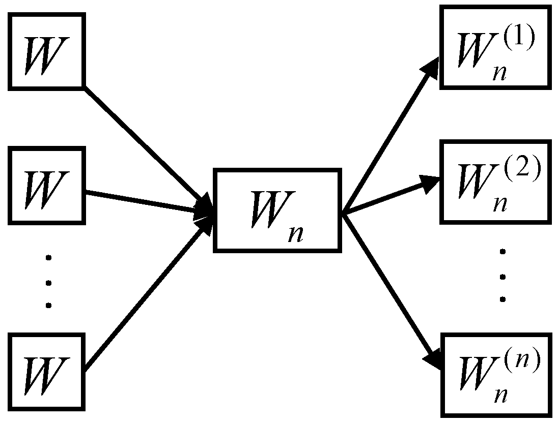
2.1. Channel Combination

When $n$ sub-channels $W$ are combined into one $W_n$ channel, the channel capacity of $W_n$ is

$$C(W_n)=I(U;Y)=I(X;Y),$$

(4)

where $U=[u_1,u_2,\cdots ,u_n]$, $Y=[y_1,y_2,\cdots ,y_n]$, and $X=[x_1,x_2,\cdots ,x_n]$. Because sub-channels are exactly the same, $u_1,u_2,\cdots ,u_n\in \{0,1\}$ are independent and identically distributed when sub-channels are B-DMC channels, and thus

$$C(W_n)=n\cdot I(X;Y)=n\cdot C(W).$$

(5)

After the channels are merged, the total capacity remains unchanged. At this time, the channel transition probability is

$$W_n(y_1^n|u_1^n)=W^n(y_1^n|u_1^n{G}_n),$$

(6)

where $y_1^n\in Y^n$, $u_1^n\in U^n$, ${\mathit{G}}_n=B_n{\mathit{F}}^{\otimes n}$, $B_n$ is the bit flip sequence, $\mathit{F}=\left[\begin{array}{cc}1& 0\\ 1& 1\end{array}\right]$, and $\otimes$ is the Kronecker product, which can be calculated as in [18].

The polar code, which completes channel combination and splitting through the corresponding coding and decoding processes, uses the channel polarization effect to realize reliable transmission. The process of channel combining is realized by polar code coding, and the index corresponding to the excellent sub-channels used to transmit information bits is called the information-bit position. Usually, $k$ information bits transmit through the first $k$ sub-channels with the largest channel capacity (that is, the smallest Bhattacharyya parameter). The index of the first $k$ sub-channels is written as $A=\{\pi \left(1\right),\pi \left(2\right),\cdots ,\pi (k\left)\right\}\in \{0,1,\cdots ,n\}$, and its complementary set is denoted as $A^c=\{0,1,\cdots ,n\}\backslash A$, so the codes with length $n$ can be written as

$$x_1^n=u_A{\mathit{G}}_n(A)\oplus u_{A^c}{\mathit{G}}_n(A^c),$$

(7)

where ${\mathit{G}}_n(A)$ is a sub-matrix of ${\mathit{G}}_n$ with index $A$, $u_A$ denoting information bits, and $u_{A^c}$ denoting frozen bits, which always takes 0, so (7) can be simplified as $x_1^n=u_A{G}_n(A)$.

The goal of blind polar recognition is to obtain the right $G_n(A)$, which is needed to obtain the code length $n$, information-bit positions $A$, and number of information bits $k$. Note that when $n$ and $k$ are determined, the rate code $R$ can be calculated as $R=k/n$.

2.2. Polar Code Construction in Gaussian Channel

The calculation of the exact value of the Bhattacharyya parameter is only applicable to the polar code construction of the BEC. It is difficult to obtain the specific value of the Bhattacharyya parameter for other channels. Usually, a GA construction algorithm with low complexity and high precision is used in AWGN; its basic idea is to approximate the log likelihood ratio (LLR) of all sub-channels to a Gaussian distribution with the mean half of the variance, gradually calculate the LLR mean of each sub-channel through the LLR mean of the total channel, and then sort the reliabilities of subchannels from smallest to largest. The LLR expressions for the channel transition probabilities are

$$\begin{array}{l}{L}_{2n}^{(2i-1)}(y_1^{2n},u_1^{2i-2})=\ln \frac{W_{2n}^{(2i-1)}(y_1^{2n},u_1^{2i-2}|u_{2i-1}=0)}{W_{2n}^{(2i-1)}(y_1^{2n},u_1^{2i-2}|u_{2i-1}=1)}=\ln \frac{{\displaystyle {\sum }_{u_{2i}^{}}{W}_n^{(i)}(y_1^n,\gamma |u_{2i-1}^{})\beta }}{{\displaystyle {\sum }_{u_{2i}^{}}{W}_n^{(i)}(y_1^n,\gamma |u_{2i-1}^{}\oplus 1)\beta }}=\\ \ln \frac{e^{L_n^{(i)}(y_1^n,\gamma )+L_n^{(i)}(y_{n+1}^{2n},u_{1,e}^{2i-2})}+1}{e^{L_n^{(i)}(y_1^n,\gamma )}+e^{L_n^{(i)}(y_{n+1}^{2n},u_{1,e}^{2i-2})}}=2{\tanh }^{-1}(\tanh \frac{L_n^{(i)}(y_1^n,\gamma )}{2}\tanh \frac{L_n^{(i)}(y_{n+1}^{2n},u_{1,e}^{2i-2})}{2})\end{array},$$

(8)

$$L_{2n}^{(2i)}(y_1^{2n},u_1^{2i-1})=\ln \frac{W_{2n}^{(2i)}(y_1^{2n},u_1^{2i-1}|u_{2i}=0)}{W_{2n}^{(2i)}(y_1^{2n},u_1^{2i-1}|u_{2i}=1)}={(-1)}^{u_{2i-1}}{L}_n^{(i)}(y_1^n,\gamma )+L_n^{(i)}(y_{n+1}^{2n},u_{1,e}^{2i-2}),$$

(9)

where $\gamma =u_{1,o}^{2i-2}\oplus u_{1,e}^{2i-2}$ and $\beta =W_n^{(i)}(y_{n+1}^{2n},u_{1,e}^{2i-2}|u_{2i}^{})$$L_1^{(i)}(y_i)=\log \frac{W(y_i|0)}{W(y_i|1)}$. When all 0 codes are transmitted, $L_1^{(i)}(y_i)~N(\frac{2}{{\sigma }^2},\frac{4}{{\sigma }^2})$, the instantaneous values of formulas (8) and (9) can be regarded as Gaussian random variables with a variance that is twice the mean value; that is, $D[L_{2n}^{(i)}]=2E[L_{2n}^{(i)}]$. $E[\cdot ]$ denotes the mean of the variable and $D[\cdot ]$ the variance of the variable, and, according to the calculation rule of [19], the following formula can be obtained:

$$E[L_{2n}^{(2i-1)}]={\varphi }^{-1}(1-{(1-\varphi (E[L_n^{(i)}]))}^2),$$

(10)

$$E[L_{2n}^{(2i)}]=2E[L_n^{(i)}],$$

(11)

where

$$\varphi (x)=\{\begin{array}{cc}1-\frac{1}{\sqrt{4\pi x}}{\displaystyle {\int }_{-\infty }^{+\infty }\tanh \frac{u}{2}{e}^{-\frac{{(u-x)}^2}{4x}}dx,}& x>0\\ 1,& x=0\end{array}.$$

(12)

The error probability for the $i^{\mathrm{th}}$ sub-channel is given approximately as [20] $Q(\sqrt{E[L_{2n}^{(i)}]/2}),1\le i\le 2n$.

3. Principle and Method of Polar Code Parameter Recognition

As the first step of channel model simulation, the simulation of polar codes in the AWGN channel has already attracted sufficient attention. According to the polar code coding structure detailed in the preceding section, the parameters that must be determined for polar code recognition under Gaussian channels include polar code length, code rate (or the number of information bits), and index of information-bit-positions. When the code length and rate are determined and the channel information known, the information-bit positions can be determined by the GA method [21], so that the generator matrix can be determined, and the channel parameters required by the GA construction method can be easily estimated by the received signal [22,23].

3.1. Recognition Principle

Theorem 1.

Denote the generator matrix of the polar code as${\mathit{G}}_n$, the set of information-bit positions as$A=\{\pi (1),\pi (2),\cdots ,\pi (k)\}$, and the new matrix${\mathit{G}}^{\prime }$is obtained after removing the ($i,i+a,\cdots ,i+c$)^th row vector, and its dual space is${\mathit{H}}_n$, if and only if$i,i+a,\cdots ,i+c\notin A$;${\mathit{H}}_n$is orthogonal to the codeword space.

Proof. 

Let ${\mathit{g}}_1,{\mathit{g}}_2,\cdots ,{\mathit{g}}_n$ represent the row vector of ${\mathit{G}}_n$. After removing row vectors with index $i,i+a,\cdots ,i+c$, ${\mathit{G}}^{\prime }$ is obtained and the space formed by the row vector in ${\mathit{G}}^{\prime }$ is ${\mathit{V}}_1=\{{\mathit{g}}_1,\cdots ,{\mathit{g}}_{i-1},{\mathit{g}}_{i+1},\cdots ,{\mathit{g}}_{i+a-1},{\mathit{g}}_{i+a+1},\cdots ,{\mathit{g}}_{i+c-1},{\mathit{g}}_{i+c+1},\cdots ,{\mathit{g}}_n\}$. The dual space of ${\mathit{G}}^{\prime }$ is ${\mathit{H}}_n=\{{\mathit{h}}_i,{\mathit{h}}_{i+a},\cdots ,{\mathit{h}}_{i+c}\}$, and the space formed by all row vectors in ${\mathit{G}}_n$ with row label in $A$ is ${\mathit{V}}_2=\{{\mathit{g}}_{\pi (1)},{\mathit{g}}_{\pi (2)},\cdots ,{\mathit{g}}_{\pi (n)}\}$. When $i,i+a,\cdots ,i+c\notin A$, ${\mathit{V}}_2\subseteq {\mathit{V}}_1$, and, therefore, ${\mathit{V}}_1^{\perp }\subseteq {\mathit{V}}_2^{\perp }$; that is, ${\mathit{H}}_n\subseteq {\mathit{V}}_2^{\perp }$, so ${\mathit{H}}_n\perp {\mathit{V}}_2$; that is, ${\mathit{H}}_n$ is orthogonal to the polar code word. If any of $i,i+a,\cdots ,i+c$ belong to the set $A$, ${\mathit{V}}_2\not\subset {\mathit{V}}_1$; that is, ${\mathit{H}}_n$ is not orthogonal to the polar code word. □

To explain the above theorem more understandably, a polar code length $n^{\prime }$ is selected to calculate generator matrix ${\mathit{G}}_{n^{\prime }}$; then, some rows are removed according to certain rules to obtain ${\mathit{G}}^{\prime }={\mathit{G}}_{n^{\prime }}(A)$. If the real code length of the codeword and the positions set of all the information bits is $A$, which can be obtained by the GA algorithm, the dual space ${\mathit{H}}_{n^{\prime }}$ is orthogonal to the intercepted codeword. This is the basic principle we use to identify polar parameters.

3.2. Model System

Assuming that $N$ polar codewords $c=[c_{1,1},c_{1,2},\cdots ,c_{1,n},\cdots ,c_{N,1},c_{N,2},\cdots ,c_{N,n}]$ with code length $n$ are transmitted, after binary phase shift keying (BPSK) modulation and utilizing the AWGN channel, its soft decision sequence $r=[r_{1,1},r_{1,2},\cdots ,r_{1,n^{\prime }},\cdots ,r_{N,1},r_{N,2},\cdots ,r_{N,n}]$ is intercepted, and then the constructed code word matrix is

$$\mathit{R}=\left[\begin{array}{cccc}{r}_{1,1}& r_{1,2}& \cdots & r_{1,n}\\ r_{2,1}& r_{2,2}& \cdots & r_{2,n}\\ ⋮& ⋮& \ddots & ⋮\\ r_{N,1}& r_{N,2}& \cdots & r_{N,n}\end{array}\right],$$

(13)

where

$$r_{i,j}=2c_{i,j}-1+n_{i,j}^{″},n_{i,j}^{″}~\mathcal{N}(0,{\sigma }^2).$$

(14)

The model system is shown in Figure 3.

The matrix formed by all the column vectors in ${\mathit{H}}_n$ is

$$\mathit{H}=\left[\begin{array}{cccc}{h}_{1,i}& h_{1,i+a}& \cdots & h_{1,i+c}\\ h_{2,i}& h_{2,i+a}& \cdots & h_{2,i+c}\\ ⋮& ⋮& \ddots & ⋮\\ h_{n,i}& h_{n,i+a}& \cdots & h_{n,i+c}\end{array}\right].$$

(15)

Let $\mathit{T}=\mathit{R}\cdot \mathit{H}$, so that

$$\mathit{T}=\left[\begin{array}{cccc}{\displaystyle \sum _{t=1}^n{r}_{1,t}{h}_{t,i}}& {\displaystyle \sum _{t=1}^n{r}_{1,t}{h}_{t,i+a}}& \cdots & {\displaystyle \sum _{t=1}^n{r}_{1,t}{h}_{t,i+c}}\\ {\displaystyle \sum _{t=1}^n{r}_{2,t}{h}_{t,i}}& {\displaystyle \sum _{t=1}^{n^{\prime }}{r}_{2,t}{h}_{t,i+a}}& \cdots & {\displaystyle \sum _{t=1}^n{r}_{2,t}{h}_{t,i+c}}\\ ⋮& ⋮& \ddots & ⋮\\ {\displaystyle \sum _{t=1}^n{r}_{n,t}{h}_{t,i}}& {\displaystyle \sum _{t=1}^n{r}_{n,t}{h}_{t,i+a}}& \cdots & {\displaystyle \sum _{t=1}^n{r}_{n,t}{h}_{t,i+c}}\end{array}\right].$$

(16)

In the ideal state, $\mathit{T}$ is an all-zero matrix—that is, the value of each element in the matrix $\mathit{T}$ is 0—but in an actual communication system, the codeword will be interfered with by noise, so even if ${\mathit{H}}_n$ is orthogonal to the original polar codeword, $\mathit{T}$ will not be an all-zero matrix. To measure whether ${\mathit{H}}_n$ is orthogonal to the original polar codeword under the AWGN channel, we consider the probability that the $K^{\mathrm{th}}$ column vector ${\mathit{h}}_K={[h_{1,K},h_{2,K},\cdots ,h_{n,K}]}^T$ in ${\mathit{H}}_n$ is orthogonal to the $i^{\mathrm{th}}$ codeword vector ${\mathit{r}}_i=[r_{i,1},r_{i,2},\cdots ,r_{i,n}]$:

$$P_{i,K}=\mathrm{Pr}({\displaystyle \sum _{t=1}^n\oplus r_{i,t}{h}_{t,K}=0|{\mathit{r}}_i}).$$

(17)

Let $l_{i,t}$ denote the LLR of $r_{i,t}$:

$$l_{i,t}=\ln (\frac{\mathrm{Pr}(c_{i,t}=0|r_{i,t})}{\mathrm{Pr}(c_{i,t}=1|r_{i,t})})=\frac{-2r_{i,t}}{{\sigma }^2}.$$

(18)

When the code weight of the $K^{\mathrm{th}}$ column vector ${\mathit{h}}_K$ is $w$ and the position of 1 in ${\mathit{h}}_K$ is $t_1,t_2,\cdots ,t_w$, the LLR of $P_{i,K}$ is

$$\begin{array}{l}A{L}_{i,K}=\ln (\frac{P_{i,K}}{1-P_{i,K}})\\ \approx \underset{t=t_1}{\overset{t_w}{\Pi }}sign(l_{i,t})\underset{t=t_1,\cdots ,t_w}{\min }(|l_{i,t}|)\end{array}.$$

(19)

Let the column numbers of ${\mathit{H}}_n$ be $N_l$; then, the average LLR of the orthogonal probabilities of $N_l$ column vectors and $N$ codewords is defined as follows:

$$AL=\frac{1}{N_l}\frac{1}{N}{\displaystyle \sum _{K=1}^{N_l}{\displaystyle \sum _{i=1}^N\mathrm{A}{\mathrm{L}}_{i,K}}}.$$

(20)

Let $\mathrm{AL}$ be the decision statistics of whether the dual space matrix ${\mathit{H}}_n$ is orthogonal to the codeword matrix $\mathit{R}$, and the following assumptions are made:

H₀: 

${\mathit{H}}_n$is not orthogonal to the codeword matrix$\mathit{R}$.

H₁: 

${\mathit{H}}_n$is orthogonal to the codeword matrix$\mathit{R}$.

All possible dual matrices for the intercepted codeword will be constructed and tested to ascertain whether any one of them satisfies the relationship between the decision statistic and decision threshold in the hypothesis test to find the dual matrix that is orthogonal to the codeword. When the correct dual matrix is found, the constructing code length and rate are considered the real parameters of the intercepted codeword, and the information-bit positions $A$ can be calculated by the GA algorithm. Then, the generator matrix can be uniquely determined, and the parameter recognition is finally realized.

Finally, the polar code parameter recognition problem is transformed into a hypothesis-testing problem, and the key is to find the decision threshold.

3.3. Decision Threshold

Let $X_i=\underset{t=t_1}{\overset{t_w}{\Pi }}sign(l_{i,t})$ and $Y_i=\underset{t=t_1,\cdots ,t_w}{\min }(|l_{i,t}|)$.

Theorem 2.

Suppose$X_1,X_2,\cdots ,X_J$are$J$independent random variables, and their distribution functions (DFs) are$F_{X_1}(x),F_{X_2}(x),\cdots ,F_{X_J}(x)$, respectively; the DF for$Z=\min \{X_1,X_2,\cdots ,X_J\}$is then

$$F_Z(z)=1-\underset{i=1}{\overset{J}{\Pi }}(1-F_{X_i}(z)).$$

(21)

The probability density function (PDF) of$Z=\min \{X_1,X_2,\cdots ,X_J\}$is

$$f_Z(z)={\displaystyle \sum _{j=1}^J{f}_{X_j}(z)}\cdot \underset{i=1,i\ne j}{\overset{J}{\Pi }}(1-F_{X_i}(z)).$$

(22)

Proof. 

From the definition of the DF, we know that

$$F_Z(z)=\mathrm{Pr}(Z\le z)=1-\mathrm{Pr}(Z>z).$$

(23)

That is to say,

$$F_Z(z)=1-\mathrm{Pr}(X_1>z)\mathrm{Pr}(X_2>z)\cdots \mathrm{Pr}(X_J>z)$$

(24)

and, in turn,

$$F_Z(z)=1-(1-\mathrm{Pr}(X_1\le z))(1-\mathrm{Pr}(X_2\le z))\cdots (1-\mathrm{Pr}(X_J\le z))$$

(25)

and

$$F_Z(z)=1-\underset{i=1}{\overset{J}{\Pi }}(1-F_{X_i}(z)).$$

(26)

Taking the derivative of $F_Z(z)$ with respect to $z$, the PDF of the random variable $Z$ is obtained as

$$f_Z(z)={\displaystyle \sum _{j=1}^J{f}_{X_j}(z)}\cdot \underset{i=1,i\ne j}{\overset{J}{\Pi }}(1-F_{X_i}(z)).$$

(27)

□

Inference 1 can be easily obtained from Theorem 2 as follows.

Inference 1.

When$X_1,X_2,\cdots ,X_J$are$J$independent and identically distributed random variables, supposing they have the same DF$F_X(x)$and PDF$f_1(x)$, then the PDF of$Z=\min \{X_1,X_2,\cdots ,X_J\}$is

$$F_Z(z)=1-{(1-F_X(z))}^J.$$

(28)

The PDF of$Z=\min \{X_1,X_2,\cdots ,X_J\}$is

$$f_Z(z)=J\cdot f_X(z)\cdot {(1-F_X(z))}^{J-1}.$$

(29)

Let $F(x)$ denote $l_{i,t}$’s DF, $f(x)$ denote $l_{i,t}$’s PDF, $F_1(x)$ denote $|l_{i,t}|$’s DF, and $f_1(x)$ denote $|l_{i,t}|$’s PDF, so

$$F_1(x)=\mathrm{Pr}(|l_{i,t}|\le x)=\mathrm{Pr}(-x\le l_{i,t}\le x),$$

(30)

where $x>0$, so

$$F_1(x)=F(x)-F(-x).$$

(31)

Taking the derivative of x on both sides of (31), we obtain

$$f_1(x)=f(x)+f(-x).$$

(32)

It can be known from (14) that

$$l_{i,j}~N(2/{\sigma }^2,4/{\sigma }^2),c_{i,j}=0,$$

(33)

$$l_{i,j}~N(-2/{\sigma }^2,4/{\sigma }^2),c_{i,j}=1.$$

(34)

$c_{i,j}$ takes the same probability of 0 and 1 without prior information, and we obtain

$$f(x)=\frac{1}{2\sqrt{2\pi }\cdot 2/\sigma }{e}^{-{(x-2/{\sigma }^2)}^2/(8/{\sigma }^2)}+\frac{1}{2\sqrt{2\pi }\cdot 2/\sigma }{e}^{-{(x+2/{\sigma }^2)}^2/(8/{\sigma }^2)}.$$

(35)

Because $f(x)=f(-x)$, when $x>0$,

$$f_1(x)=\frac{\sigma }{2\sqrt{2\pi }}{e}^{-{\sigma }^2{(x-2/{\sigma }^2)}^2/8}+\frac{\sigma }{2\sqrt{2\pi }}{e}^{-{\sigma }^2{(x+2/{\sigma }^2)}^2/8}.$$

(36)

When $x\le 0$, $f_1(x)=0$.

Let $f_2(x)$ be the PDF of $Y_i$, and then it is known from Inference 1 that

$$f_2(x)=\{\begin{array}{cc}w\cdot f_1(x)\cdot {(1-F_1(x))}^{w-1}& ,x>0\\ 0& ,x\le 0\end{array}.$$

(37)

Thus, the expectation of $Y_i$ and $Y_i^2$ can be obtained, respectively, as

$$E(Y_i)={\int }_0^{+\infty }w\cdot x\cdot f_1(x)\cdot {(1-F_1(x))}^{w-1}dx,$$

(38)

$$E(Y_i^2)={\int }_0^{+\infty }w\cdot x^2\cdot f_1(x)\cdot {(1-F_1(x))}^{w-1}dx.$$

(39)

Calculating integration by parts,

$$E(Y_i)={-x\cdot {(1-F_1(x))}^w|}_0^{+\infty }+{\int }_0^{+\infty }{(1-F_1(x))}^{w}dx,$$

(40)

$$E(Y_i^2)={-x^2\cdot {(1-F_1(x))}^w|}_0^{+\infty }+{\int }_0^{+\infty }2x\cdot {(1-F_1(x))}^{w}dx.$$

(41)

According to the L’Hospital principle $\underset{x\to +\infty }{\lim }x(1-F_1(x))=0$,

$\underset{x\to +\infty }{\lim }{x}^2(1-F_1(x))=0$, so (40) and (41) can be rewritten, respectively, as

$$E(Y_i)={\int }_0^{+\infty }{(1-F_1(x))}^{w}dx,$$

(42)

$$E(Y_i^2)={\int }_0^{+\infty }2x\cdot {(1-F_1(x))}^{w}dx,$$

(43)

where $F_1(x)={\int }_0^x{f}_1(t)dt$, so

$$F_1(x)=0.5(erf(\frac{x+\frac{2}{{\sigma }^2}}{\frac{2\sqrt{2}}{\sigma }})+erf(\frac{x-\frac{2}{{\sigma }^2}}{\frac{2\sqrt{2}}{\sigma }})),$$

(44)

where $erf(x)=\frac{2}{\sqrt{\pi }}{\int }_0^x{e}^{-t^2}$.

It is easy to know that $X_i^2\cdot Y_i^2=Y_i^2$ and it has nothing to do with the assumptions, so

$$E(Y_i^2)=E(X_i^2\cdot Y_i^2|H_0)=E(X_i^2\cdot Y_i^2|H_1).$$

(45)

If $H_0$ is true, ${\mathit{h}}_K$ is not orthogonal to the codeword, so

$$E(X_i\cdot Y_i^{}|H_0)=0,$$

(46)

$$Var(X_i\cdot Y_i|H_0)=E(X_i^2\cdot Y_i^2|H_0)={\int }_0^{+\infty }2x\cdot {(1-F_1(x))}^{w}dx.$$

(47)

If $H_1$ is true, and the judgment of $c_{i,t}$ is correct, let $R_1$ denote the condition of $c_{i,t}=0$, $l_{i,t}>0$ and $R_2$ denote the condition of $c_{i,t}=1$, $l_{i,t}<0$; then, the PDFs of $l_{i,t}$ are

$$f(x|R_1)=\{\begin{array}{cc}\frac{\sigma \cdot e^{-{\sigma }^2\cdot {(x-2/{\sigma }^2)}^2/8}}{\sqrt{2\pi }(1+erf(1/(\sqrt{2}\sigma )))}& ,x>0\\ 0& ,x\le 0\end{array},$$

(48)

$$f(x|R_2)=\{\begin{array}{cc}\frac{\sigma \cdot e^{-{\sigma }^2\cdot {(x+2/{\sigma }^2)}^2/8}}{\sqrt{2\pi }(1+erf(1/(\sqrt{2}\sigma )))}& ,x<0\\ 0& ,x\ge 0\end{array}.$$

(49)

Let $F(x|R_1)$ and $F(x|R_2)$ denote the cumulative functions (CFs) of $f(x|R_1)$ and $f(x|R_2)$, respectively, so the CFs of $Y=|l_{i,t}|$ are

$$F_Y(y|R_1)=\{\begin{array}{cc}F(y|R_1)-F(-y|R_1)& ,y>0\\ 0& ,y\le 0\end{array},$$

(50)

$$F_Y(y|R_2)=\mathrm{Pr}(Y\le y|R_2)=\{\begin{array}{cc}F(y|R_2)-F(-y|R_2)& ,y>0\\ 0& ,y\le 0\end{array}.$$

(51)

When $y>0$, $F(-y|R_1)=0$, and $F(y|R_2)=1$, so $F_Y(y|R_1)=F(y|R_1)$ and $F_Y(y|R_2)=1-F(-y|R_2)$, and therefore the PDFs of $Y$ are

$$f_Y(y|R_1)=\{\begin{array}{cc}f(y|R_1)& ,y>0\\ 0& ,y\le 0\end{array},$$

(52)

$$f_Y(y|R_2)=\{\begin{array}{cc}f(-y|R_2)& ,y>0\\ 0& ,y\le 0\end{array}.$$

(53)

It can be obtained from (49), (50), (53), and (54) that, when $y\ge 0$, $f_Y(y|R_1\cup R_2)=0$, and, when $y<0$, that

$$f_Y(y|R_1\cup R_2)=\frac{\sigma \cdot e^{-{\sigma }^2\cdot {(y-2/{\sigma }^2)}^2/8}}{\sqrt{2\pi }(1+erf(1/(\sqrt{2}\sigma )))}.$$

(54)

If $H_1$ is true, and the judgment of $c_{i,t}$ is not correct, let $R_1^{\prime }$ denote the condition of $c_{i,t}=0,l_{i,t}<0$ and $R_2^{\prime }$ denote the condition of $c_{i,t}=1,l_{i,t}>0$; then, the PDFs of $l_{i,t}$ are

$$f(x|R_1^{\prime })=\{\begin{array}{cc}\frac{\sigma \cdot e^{-{\sigma }^2\cdot {(x-2/{\sigma }^2)}^2/8}}{\sqrt{2\pi }(1-erf(1/(\sqrt{2}\sigma )))}& ,x>0\\ 0& ,x\le 0\end{array},$$

(55)

$$f(x|R_2^{\prime })=\{\begin{array}{cc}\frac{\sigma \cdot e^{-{\sigma }^2\cdot {(x+2/{\sigma }^2)}^2/8}}{\sqrt{2\pi }(1-erf(1/(\sqrt{2}\sigma )))}& ,x>0\\ 0& ,x\le 0\end{array},$$

(56)

and the PDFs of Y are

$$f_Y(y|R_1^{\prime })=\{\begin{array}{cc}f(-y|R_1^{\prime })& ,y>0\\ 0& ,y\le 0\end{array},$$

(57)

$$f_Y(y|R_2^{\prime })=\{\begin{array}{cc}f(y|R_2^{\prime })& ,y>0\\ 0& ,y\le 0\end{array}.$$

(58)

It can be obtained from (55)–(58) that, when $y\le 0$, $f_Y(y|R_1^{\prime }\cup R_2^{\prime })=0$, and, when $y>0$, that

$$f_Y(y|R_1^{\prime }\cup R_2^{\prime })=\frac{\sigma \cdot e^{-{\sigma }^2\cdot {(y+2/{\sigma }^2)}^2/8}}{\sqrt{2\pi }(1-erf(1/(\sqrt{2}\sigma )))}.$$

(59)

Assuming that there is an error in the element at position $\{t_{v_1},t_{v_2},\cdots ,t_{v_s}\}$ in $l_{i,t_1},l_{i,t_2},\cdots ,l_{i,t_w}$, it is easy to obtain the set of correct element positions as $\{t_{j_1},t_{j_2},\cdots ,t_{j_{w-s}}\}=\{t_1,t_2,\cdots ,t_w\}/\{t_{v_1},t_{v_2},\cdots ,t_{v_s}\}$. Letting $T_1^s=\min \{|l_{i,t_{v_1}}|,|l_{i,t_{v_2}}|,\cdots ,|l_{i,t_{v_s}}|\}$ and $T_2^s=\min \{|l_{i,t_{j_1}}|,|l_{i,t_{j_2}}|,\cdots ,|l_{i,t_{j_{w-s}}}|\}$, it can be obtained from Inference 2-1 that, when $y\le 0$, $f_{T_1^s}(y)=0$ and $f_{T_2^s}(y)=0$, and, when $y>0$, that

$$f_{T_1^s}(y)=s\cdot f_Y(y|R_1^{\prime }\cup R_2^{\prime }){(1-F_Y(y|R_1^{\prime }\cup R_2^{\prime }))}^{s-1},$$

(60)

$$f_{T_2^s}(y)=(w-s)\cdot f_Y(y|R_1^{}\cup R_2^{}){(1-F_Y(y|R_1^{}\cup R_2^{}))}^{w-s-1},$$

(61)

where $F_Y(y|R_1^{\prime }\cup R_2^{\prime })$ and $F_Y(y|R_1^{}\cup R_2^{})$ are the CFs of $f_Y(y|R_1^{\prime }\cup R_2^{\prime })$ and $f_Y(y|R_1^{}\cup R_2^{})$, respectively, so that, when $y>0$,

$$\begin{array}{l}{F}_Y(y|R_1^{\prime }\cup R_2^{\prime })={\int }_0^y{f}_Y(t|R_1^{\prime }\cup R_2^{\prime })dt=\\ \frac{1}{1-erf(1/(\sqrt{2}\sigma ))}·(erf(\frac{y\sigma }{2\sqrt{2}}+\frac{1}{\sqrt{2}\sigma })+erf(\frac{1}{\sqrt{2}\sigma }))\end{array},$$

(62)

$$\begin{array}{l}{F}_Y(y|R_1^{}\cup R_2^{})={\int }_0^y{f}_Y(t|R_1^{}\cup R_2^{})dt=\\ \frac{1}{1+erf(1/(\sqrt{2}\sigma ))}(erf(\frac{y\sigma }{2\sqrt{2}}-\frac{1}{\sqrt{2}\sigma })+erf(\frac{1}{\sqrt{2}\sigma }))\end{array}.$$

(63)

Letting $T^s=\min \{T_1^s,T_2^s\}$, from Theorem 2 we can obtain

$$f_{T_{}^s}(y)=f_{T_1^s}(y)\cdot (1-F_{T_2^s}(y))+f_{T_2^s}(y)\cdot (1-F_{T_1^s}(y)),$$

(64)

where $F_{T_1^s}(y)$ and $F_{T_2^s}(y)$ are the CFs of $f_{T_1^s}(y)$ and $f_{T_2^s}(y)$, respectively; that is,

$$F_{T_1^s}(y)=\{\begin{array}{cc}1-{(1-F_Y(y|R_1^{\prime }\cup R_2^{\prime }))}^s& ,y>0\\ 0& ,y\le 0\end{array},$$

(65)

$$F_{T_2^s}(y)=\{\begin{array}{cc}1-{(1-F_Y(y|R_1^{}\cup R_2^{}))}^{w-s}& ,y>0\\ 0& ,y\le 0\end{array}.$$

(66)

When $X_i=1$, the number of error symbols is even and the check relationship is still established, so

$$E(X_i\cdot Y_i,X_i=1|H_1)={\displaystyle \sum _{i=0}^{\lfloor w/2\rfloor }{C}_w^{2i}{p}_e^{2i}{(1-p_e)}^{w-2i}}\underset{0}{\overset{+\infty }{\int }}x{f}_{T^{2i}}(x)dx,$$

(67)

where $p_e$ is the theoretical bit error rate of the codewords modulated by BPSK, and the expression is

$$p_e=0.5erfc(\sqrt{1/(2{\sigma }^2)}),$$

(68)

where ${\sigma }^2$ is noise variance, $erfc(x)=\frac{2}{\sqrt{\pi }}\underset{-\infty }{\overset{x}{\int }}{e}^{-t^2}dt$.

Similarly, when $X_i=-1$, an odd number of errors occurs:

$$E(X_i\cdot Y_i,X_i=-1|H_1)=-{\displaystyle \sum _{i=0}^{\lfloor w/2\rfloor -1}{C}_w^{2i+1}{p}_e^{2i+1}{(1-p_e)}^{w-2i-1}}·{\displaystyle \underset{0}{\overset{+\infty }{\int }}x{f}_{T^{2i+1}}(x)dx}.$$

(69)

It can be obtained from (67) and (69) that

$$E(X_i\cdot Y_i|H_1)=E(X_i\cdot Y_i,X_i=1|H_1)+E(X_i\cdot Y_i,X_i=-1|H_1),$$

(70)

$$Var(X_i\cdot Y_i|H_1)=E(Y_i^2)-E{(X_i\cdot Y_i|H_1)}^2.$$

(71)

It is easy to obtain the mean and variance of $\mathrm{A}{\mathrm{L}}_{i,k}$ under the two assumptions:

$$E(\mathrm{A}{\mathrm{L}}_{i,k}|H_0)=E(X_i\cdot Y_i|H_0)=0,$$

(72)

$$E(\mathrm{A}{\mathrm{L}}_{i,k}|H_1)=E(X_i\cdot Y_i|H_1),$$

(73)

$$Var(\mathrm{A}{\mathrm{L}}_{i,k}|H_0)=Var(X_i\cdot Y_i|H_0),$$

(74)

$$Var(\mathrm{A}{\mathrm{L}}_{i,k}|H_1)=Var(X_i\cdot Y_i|H_1).$$

(75)

According to the statistical properties of random variables,

$${\mu }_0=E(\mathrm{A}\mathrm{L}|H_0)=E(\mathrm{A}{\mathrm{L}}_{i,k}|H_0)=0,$$

(76)

$${\mu }_1=E(\mathrm{A}\mathrm{L}|H_1)=E(\mathrm{A}{\mathrm{L}}_{i,k}|H_1),$$

(77)

$${\sigma }_0^2=Var(\mathrm{A}\mathrm{L}|H_0)=Var(\mathrm{A}{\mathrm{L}}_{i,k}|H_0)/N/N_l,$$

(78)

$${\sigma }_1^2=Var(\mathrm{A}\mathrm{L}|H_1)=Var(\mathrm{A}{\mathrm{L}}_{i,k}|H_1)/N/N_l.$$

(79)

Then, the false alarm probability is

$$P_f={\int }_{\Lambda }^{+\infty }\frac{1}{\sqrt{2\pi }{\sigma }_0}{e}^{\frac{-{(x-{\mu }_0)}^2}{2{\sigma }_0^2}}dx.$$

(80)

The probability of a false alarm is

$$P_a={\int }_{-\infty }^{\Lambda }\frac{1}{\sqrt{2\pi }{\sigma }_1}{e}^{\frac{-{(x-{\mu }_1)}^2}{2{\sigma }_1^2}}dx.$$

(81)

It does not have any prior knowledge under non-cooperative conditions, so $P_f=P_a$, and the average incorrect decision probability is

$$P_{er}=0.5P_f+0.5P_a={\int }_{\Lambda }^{+\infty }\frac{1}{\sqrt{2\pi }{\sigma }_0}{e}^{\frac{-{(x-{\mu }_0)}^2}{2{\sigma }_0^2}}dx+{\int }_{-\infty }^{\Lambda }\frac{1}{\sqrt{2\pi }{\sigma }_1}{e}^{\frac{-{(x-{\mu }_1)}^2}{2{\sigma }_1^2}}dx.$$

(82)

The minimum error decision threshold for solving (82) is

$${\Lambda }_{\mathrm{opt}}=\frac{({\sigma }_0^2\cdot {\mu }_1-{\sigma }_1^2\cdot {\mu }_0)-{\sigma }_0{\sigma }_1\cdot \zeta }{({\sigma }_0^2-{\sigma }_1^2)},$$

(83)

where $\zeta =\sqrt{{({\mu }_0-{\mu }_1)}^2+({\sigma }_1^2-{\sigma }_0^2)\cdot \ln ({\sigma }_1/{\sigma }_0)}$. When $\mathrm{AL}>{\Lambda }_{\mathrm{opt}}$, $H_1$ is true.

3.4. Parameter Recognition Steps

Since 3GPP stipulates that the maximum mother code length of the polar code in the downlink control information is 512, that in the uplink control information is 1024 [24]. Considering the code length and code-rate range of polar codes in practical applications, the code length is selected as $n^{″}=[32,64,128,256,512,1024]$ and the algorithm code rate is selected as $R^{″}=[\frac{1}{5},\frac{1}{3},\frac{2}{5},\frac{1}{2},\frac{2}{3},\frac{3}{4},\frac{5}{6},\frac{8}{9}]$ for the polar code simulation in this paper. The range of the signal-to-noise (SNR) ratio is $-4\le SNR\le 6$. Denoting the total number of program executions as $L$, and the times of $\mathrm{AL}>{\Lambda }_{\mathrm{opt}}$ under a certain code length, code rate, information-bit position, and signal-to-noise ratio during the execution process as $\mathrm{Num}$, we then define the polar code recognition conformity $\eta$ as follows:

$$\eta =\frac{\mathrm{Num}}{L}.$$

(84)

According to the definition of $\eta$, when the code length, code rate, and information-bit positions used in constructing ${\mathit{H}}_n$ are completely consistent with the transmitted codeword, $\eta$ takes the maximum value. The specific algorithm is shown as Algorithm 1.

Algorithm 1: Polar code parameter recognition

$\mathbf{Input}:n^{″}$; $R^{″}$; soft decision sequence $r$; numbers of code length, $N_n$; numbers of code rate, $N_r$; execution numbers $L$

$\mathbf{Output}:\widehat{n}$$,\widehat{R}$$,\widehat{A}$

$\mathbf{Initialization}:\mathrm{Num}=\mathrm{zeros}(N_n,N_r)$$,j=0$

1   $\mathbf{for}{n}^{\prime }=n^{″}$ do

2     $\mathrm{Construct}\mathrm{codeword}\mathrm{matrix}\mathit{R}$;

3     $\mathbf{for}{R}^{\prime }=R^{″}$ do

4       $j=j+1$;

5       $\mathrm{construct}{A}^{\prime }$$\mathrm{by}\mathrm{GA}\mathrm{algorithm}\mathrm{with}{n}^{\prime }$$,R^{\prime }$;

6       $\mathrm{construct}{\mathit{G}}_{n^{\prime }}(A^{\prime })$$\mathrm{with}{n}^{\prime }$$,R^{\prime }$$,\mathrm{and}{A}^{\prime }$$;\mathrm{calculate}{\mathit{H}}_{n^{\prime }}$;

7       $\mathrm{get}\mathrm{statistics}\mathrm{AL}$$\mathrm{and}\mathrm{threshold}{\Lambda }_{\mathrm{opt}}$;

8       $\mathbf{if}\mathrm{AL}<{\Lambda }_{\mathrm{opt}}$ then

9         $\mathrm{Num}(j)=\mathrm{Num}(j)+1$;

10         $\eta (j)=\mathrm{Num}(j)/\mathrm{L}$;

11     end if

12    end for

13  end for

14  $\mathrm{Find}\mathrm{all}j$$\mathrm{that}\mathrm{make}\eta$$\mathrm{take}\mathrm{the}\mathrm{maximum}\mathrm{value};\mathrm{number}\mathrm{of}j$$\mathrm{is}lenj$;

15  $\mathbf{for}i=1$ $\mathrm{to}i=lenj$ do

16    $p1=\mathrm{mod}(j,N_r),p2=fix(j,N_r)$;

17    $\mathbf{if}p1=0$ then

18      $R^{\prime }(i)=8/9$;

19    else

20      $R^{\prime }(i)=R(p2)$;

21    end if

22    $n^{\prime }(i)=n(p1+1)$;

23  end for

24  $\widehat{n}=\min (n^{\prime })$$,\widehat{R}=\min (R^{\prime })$$,\mathrm{construct}\widehat{A}$$\mathrm{by}\mathrm{GA}\mathrm{with}\widehat{n}$$,\widehat{R}$;

25  $\mathrm{return}\widehat{n}$$,\widehat{R}$$,\widehat{A}$

4. Numerical Simulation

We first examined the algorithm validity and then executed the recognition algorithm presented in Section 3.4 to examine the influence of different factors. Then, the performance and complexity were compared with that of the algorithm presented in [15,16]. Unless otherwise stated, the simulation takes the same parameters as in Section 3.4. Since this paper examines the problem of polar code parameter recognition under the AWGN channel, the simulations here were confined to the AWGN channel.

4.1. Algorithm-Validity Verification

Algorithm validity was evaluated in two cases: (1) with polar code length 256, code rate 1/2, and SNR = 30 dB, and (2) with polar code length 256, code rate 2/3, and number of transmitted codewords 2000. The results of the average likelihood ratio (LLR) and threshold are presented in Figure 4 and Figure 5.

As shown in both figures, the abscissa “Oder” corresponds to $j$ in Algorithm 1, so the code length and rate corresponding to each abscissa can be calculated according to Section 3.4. For example, when the abscissa is 38, the average LLR exceeds the threshold for the third time and the total number of code rates is 8. It is easy to calculate that $38÷8=4\cdots \cdots 6$, so the corresponding code rate is the sixth $R^{″}$, $\frac{3}{4}$, and the code length is the 4 + 1, or fifth, $n^{″}$, 256. It can be seen from the figures that when the code length and rate are not lower than the real code length and rate, respectively, the code length and rate will be mistakenly identified as the real polar code parameters. This is due to the channel polarization effect, which guarantees a certain structural relationship between a polar code and polar codes in which the code length and rate are not lower than this code. Therefore, we selected the minimum code length and rate corresponding to the maximum $\eta$ as the final result.

4.2. Influence of Code Rate

A recognition rate with lengths of 128, 256, and 512 is simulated when the code rate is different. The number of codewords was 2000, the recognition rate was output every 0.5 dB, and 2000 Monte Carlo calculations were performed. The results are shown in Figure 6, Figure 7 and Figure 8.

As shown in the figures, when the code rate decreases, the recognition performance is improved, but this performance improvement decreases with increasing code length. This is because when the code length is constant, the dimension of the dual space increases as the code rate decreases, and the calculation of the statistic is closer to the theoretical value, so the recognition performance is improved. Otherwise, the increase in the code length will increase the total code weight of the dual-space vector, making the calculation of the statistic more susceptible to bit errors. This slowly offsets the performance improvement brought about by the reduction of the code rate. The longer the code length, the more obvious the offset, and the recognition performance curves of different code rates become increasingly closer.

4.3. Influence of Intercepted Codewords

Recognition rate curves under different numbers of codewords were simulated with code rate 1/2, code length 64, and SNR range −2–4 dB. The recognition rate was output once every 0.5 dB and 1000 Monte Carlo calculations performed. The results are shown in Figure 9.

As shown in the figure, with the increasing number of codewords, the recognition performance of the algorithm continues to improve, but the degree of improvement is increasingly lower. This is because the continuous increase in the number of codewords makes the statistic approach the theoretical value gradually; the closer to the theoretical value, the less the performance improvement.

4.4. Influence of Code Length

The recognition rate curve of the proposed algorithm was simulated under different code lengths with 1/3 code rate, 2000 codewords, the SNR range of −2–8 dB, and the recognition rate output every 0.5 dB. The results of 2000 simulations are shown in Figure 10.

As shown in the figure, as the code length increases, the recognition performance of the algorithm deteriorates. This is because the longer the code length and the larger the code weight, the more easily the accuracy of the statistic calculation is affected by bit errors, and thus the recognition performance decreases.

4.5. Comparison of Recognition Performance

In this section, we compared the recognition performance of the proposed algorithm with that of algorithms in [15,16], which also studied polar code parameter recognition under the AWGN channel in recent years. All the algorithms are executed with structured and unstructured polar codes with a code length of 256 and a code rate of 1/3 and 2000 codewords, and the results are shown as follows. The curves of the algorithm proposed in this study are marked as DS, and those of the algorithms advanced in [15,16] are marked as [15,16] in Figure 11, Figure 12 and Figure 13.

As shown in the figures, when the parameters of structured polar codes are recognized, the recognition performance of the algorithm proposed in this paper is better than that of the algorithm advanced in [15] and worse than that in [16]. This is because the algorithm advanced in [15] identifies the information bit positions one by one, which makes it insensitive to the coding structure, and it suffers from errors involving correct information bit numbers but incorrect bit positions. The algorithm proposed in this paper directly uses the GA construction method to determine the number and distribution of the information-bit index, which means that when the code length and rate are correctly identified, the information-bit index must be correct. This helps avoid the recognition error with a correct information-bit number with an incorrect index, while at the same time avoiding calculating the judgment statistic row by row and reducing the number of calculations. The computation comparison is analyzed in detail in the following subsection, and the introduction of likelihood difference in [16] did boost performance.

However, the algorithms advanced in [15,16] are invalid when recognizing the parameters of structured polar codes. This is because the recognition criteria of algorithms advanced in [15,16] are only designed for structured polar codes, so they failed in terms of unstructured polar code recognition.

4.6. Algorithm Complexity

Setting the amount of intercepted data as $\mathrm{Len}$, when the traversal calculation reaches the code length $n^{\prime }$$(n_{\min }\le n^{\prime }\le n_{\max })$ and the code rate $R^{\prime }$$(R_{\min }\le R^{\prime }\le R_{\max })$, the dual matrix $\mathit{H}$ is calculated after removing the $n^{\prime }(1-R^{\prime })$ rows in the construction matrix ${\mathit{G}}_{n^{\prime }}$; then, the statistics $\mathrm{AL}$ and thresholds ${\Lambda }_{\mathrm{opt}}$ of $\lfloor \mathrm{Len}/n^{\prime }\rfloor$ codewords are calculated. The dual matrix with fixed code length and rate is fixed, so it can be generated in advance and read directly when needed. The calculation of statistics requires $\lfloor \mathrm{Len}/n^{\prime }\rfloor \cdot n^{\prime }(1-R^{\prime })$ vector additions, $\lfloor \mathrm{Len}/n^{\prime }\rfloor \cdot n^{\prime }(1-R^{\prime })$ comparisons, and $\lfloor \mathrm{Len}/n^{\prime }\rfloor \cdot n^{\prime }(1-R^{\prime })$ vector multiplications. For simplicity, one comparison is equivalent to one vector addition, so the number of addition computations of the parameter recognition algorithm proposed in this paper is ${\displaystyle \sum _{R^{\prime }=R_{\min }}^{R^{\prime }=R_{\max }}{\displaystyle \sum _{n^{\prime }=n_{\min }}^{n^{\prime }=n_{\max }}2\lfloor \mathrm{Len}/n^{\prime }\rfloor \cdot n^{\prime }(1-R^{\prime })}}$ and the number of multiplications is ${\displaystyle \sum _{R^{\prime }=R_{\min }}^{R^{\prime }=R_{\max }}{\displaystyle \sum _{n^{\prime }=n_{\min }}^{n^{\prime }=n_{\max }}\lfloor \mathrm{Len}/n^{\prime }\rfloor \cdot n^{\prime }(1-R^{\prime })}}$. Therefore, the complexity of the algorithm proposed in this paper approximately increases linearly with increasing length of the intercepted data and decreasing code rate. Regarding the algorithm proposed in [15], the number of multiplications is ${\displaystyle \sum _{n^{\prime }=n_{\min }}^{n^{\prime }=n_{\max }}20\cdot n^{\prime }}$, the number of additions is ${\displaystyle \sum _{n^{\prime }=n_{\min }}^{n^{\prime }=n_{\max }}\mathrm{Len}\cdot n^{\prime }}$, and the calculation amount increases approximately linearly with increasing length of the intercepted data and code length. The algorithm proposed in [16] requires at most $5\cdot \mathrm{Len}+10\cdot n^{\prime }+(2\cdot n^{\prime }-1)\cdot \mathrm{Len}$ multiplications and $(\mathrm{Len}/(2\cdot n^{\prime })-1)\cdot {(2\cdot n^{\prime })}^2$ additions. Let the sum of the number of multiplications and additions be the complexity, and we show how code length, code rate, and the received sequence length influence the complexity in what follows. When the influence of code length and code rate on complexity is considered, the length of the received sequence length is set to 10,000. When the influence of sequence length on complexity is considered, a code length of 512 and a code rate of 1/2 are chosen.

As is shown in Figure 12, the complexities of the algorithms proposed in [15,16] are not affected by code rate so they just have one curve, but the complexity of the algorithm proposed in this paper is affected by code rate, so the complexity with every code rate has a curve. All the complexities increase as the code length increases from 32 to 1024, but the complexity of the algorithm proposed in this paper increases only when the code rate increases from 1/5 to 8/9. As shown in Figure 13, all the complexities increase as the sequence length increases from 2000 to 10,000. Regardless, the complexity of the algorithm proposed in this paper is the lowest.

5. Conclusions

To reduce the complexity and improve the performance of a polar code parameter recognition algorithm, a traditional recognition scheme suitable for blind recognition of polar code parameters in AWGN channels is proposed in this paper. The hypothesis test of the empirical relationship is studied, the specific calculation process of statistics and decision thresholds is given, and the effectiveness of the proposed algorithm and the conditions of different code lengths, code rates, and number of received codewords are simulated. Simulation results show that the recognition performance of the algorithm proposed in this paper increases with the decreasing code length, increasing number of intercepted codewords, and decreasing code rate.

Compared with the existing algorithms for AWGN channel simulation, the algorithm proposed in this paper not only has the lowest simulation complexity, but also has good recognition performance. More importantly, it is valid for unstructured polar codes, making it outperform other algorithms. The research results in this paper can be applied to simulation implementations in the fields of intelligent communication, communication reconnaissance, and network countermeasures. In the future, we will study the problem of polar code parameter recognition under other channels and consider adding machine-learning algorithms to our studies.

References

1. Arikan, E. Channel polarization: A method for constructing capacity-achieving codes for symmetric binary-input memoryless channels. IEEE Trans. Inf. Theory 2009, 55, 3051–3073. [Google Scholar] [CrossRef]
2. Gamage, H.; Rajatheva, N.; Latva-Aho, M. Channel coding for enhanced mobile broadband communication in 5G systems. In Proceedings of the 2017 European Conference on Networks and Communications, Oulu, Finland, 12–15 June 2017; pp. 1–6. [Google Scholar]
3. Abusabah, I.A.A.; Abdeldafia, M.; Abdelaziz, Y.M.A. Blind Identification of Convolutional Codes Based on Veterbi Algorithm. In Proceedings of the 2020 International Conference on Computer, Control, Electrical, and Electronics Engineering (ICCCEEE), Khartoum, Sudan, 26 February–1 March 2021; pp. 1–4. [Google Scholar]
4. Huang, L.; Chen, W.; Chen, E.; Chen, H. Blind recognition of k/n rate convolutional encoders from noisy observation. J. Syst. Eng. Electron. 2017, 28, 235–243. [Google Scholar]
5. Li, L.Q.; Huang, Z.; Zhou, J. Blind identification of LDPC codes based on a candidate set. IEEE Commun. Lett. 2021, 25, 2786–2789. [Google Scholar]
6. Lei, Y.; Luo, L. Novel Blind Identification of LDPC Code Check Vector Using Soft-decision. In Proceedings of the 2020 IEEE 20th International Conference on Communication Technology (ICCT), Nanning, China, 28–31 October 2020; pp. 1291–1295. [Google Scholar]
7. Wu, Z.J.; Zhang, L.M.; Zhong, Z.G.; Liu, R.X. Blind recognition of LDPC codes over candidate set. IEEE Commun. Lett. 2020, 24, 11–14. [Google Scholar] [CrossRef]
8. Swaminathan, R.; Madhukumar, A.S.; Wang, G.H. Blind estimation of code parameters for product codes over noisy channel conditions. IEEE Trans. Aerosp. Electron. Syst. 2020, 56, 1460–1473. [Google Scholar] [CrossRef]
9. Wu, Z.J.; Zhang, L.M.; Zhong, Z.G. A maximum cosinoidal cost function method for parameter estimation of RSC turbo codes. IEEE Commun. Lett. 2019, 23, 390–393. [Google Scholar]
10. Wand, J.; Tang, C.R.; Huang, H.; Wang, H.; Li, J.Q. Blind identification of convolutional codes based on deep learning. Digit Signal Process. 2021, 115, 103086. [Google Scholar]
11. Chen, J.J. Research and Implementation of Closed Set Recognition of Error Correction Coding Based on Deep Learning. Master’s Thesis, University of Electronic Science and Technology of China, Chengdu, China, 2020. [Google Scholar]
12. Chen, C. Recognition of Closed Set Turbo Codes Based on Machine Learning. Master’s Thesis, University of Electronic Science and Technology of China, Chengdu, China, 2020. [Google Scholar]
13. Liu, J.; Zhang, L.M.; Zhong, Z.G. Blind parameter identification of RS code based on binary field equivalence. Acta Electron. Sin. 2018, 46, 2888–2894. [Google Scholar]
14. Zhang, T.Q.; Hu, Y.P.; Feng, J.X.; Zhang, X.Y. Blind algorithm of polarization code parameters based on null space matrix matching. J. Electr. Eng. Technol. 2020, 42, 2953–2959. [Google Scholar]
15. Wu, Z.J.; Zhong, Z.G.; Zhang, L.M.; Dan, B. Recognition of non-drilled polar codes based on soft decision. J. Commun. 2020, 41, 60–71. [Google Scholar]
16. Wang, Y.; Wang, X.; Yang, G.D.; Huang, Z. Recognition algorithm of non punctured polarization codes based on structural characteristics of coding matrix. J. Commun. 2022, 43, 22–33. [Google Scholar]
17. Xu, J.; Yuan, Y.F. Channel Coding for New Radio of 5th Generation Mobile Communications; Posts & Telecom Press: Beijing, China, 2018. [Google Scholar]
18. John, W.B. Kronecker Products and matrix calculus in system theory. IEEE Trans. Circuits Syst. 1978, 25, 772–781. [Google Scholar]
19. Melnikov, N.B.; Reser, B.I. Gaussian Approximation. In Dynamic Spin-Fluctuation Theory of Metallic Magnetism, 1st ed.; Springer International Publishing AG: Cham, Switzerland, 2018; pp. 101–108. [Google Scholar]
20. Proakis, J.G. Digital Communications; McGraw Hill: New York, NY, USA, 1995. [Google Scholar]
21. Trifonov, P. Efficient design and decoding of polar codes. IEEE Trans. Commun. 2012, 60, 3221–3227. [Google Scholar] [CrossRef]
22. Zimaglia, E.; Riviello, D.G.; Garello, R.; Fantini, R. A Deep Learning-based Approach to 5G-New Radio Channel Estimation. In Proceedings of the 2021 Joint European Conference on Networks and Communications & 6G Summit, Porto, Portugal, 8–11 June 2021; pp. 1–6. [Google Scholar]
23. Pauluzzi, D.R.; Beaulieu, N.C. A comparison of SNR estimation techniques for the AWGN channel. IEEE Trans. Commun. 2000, 48, 1681–1691. [Google Scholar] [CrossRef]
24. 3GPP. Study on New Radio Access Technology Physical Layer Aspects (Release 14), TR 38.802 V14.1.0[R]. 2017, pp. 14–43. Available online: http://www.3gpp.org (accessed on 27 April 2007).
Figure 1. Diagram of channel.
Electronics 11 02511 g001
Figure 2. Diagram of channel combination and separation.
Electronics 11 02511 g002
Figure 3. Model system.
Electronics 11 02511 g003
Figure 4. Algorithm-validity verification with 5 dB.
Electronics 11 02511 g004
Figure 5. Algorithm-validity verification with 30 dB.
Electronics 11 02511 g005
Figure 6. Recognition performance under different code rates with code length 128.
Electronics 11 02511 g006
Figure 7. Recognition performance under different code rates with code length 256.
Electronics 11 02511 g007
Figure 8. Recognition performance under different code rates with code length 512.
Electronics 11 02511 g008
Figure 9. Performance under different number of codewords.
Electronics 11 02511 g009
Figure 10. Performance under different code lengths.
Electronics 11 02511 g010
Figure 11. Comparison of recognition performance under different code lengths [15,16]. (a) The curves under structured polar codes. (b) The curves under unstructured polar codes.
Electronics 11 02511 g011
Figure 12. Influence of code length and code rate on complexity [15,16].
Electronics 11 02511 g012
Figure 13. Influence of sequence length on complexity [15,16].
Electronics 11 02511 g013
Publisher’s Note: MDPI stays neutral with regard to jurisdictional claims in published maps and institutional affiliations.