An Intelligent Identification Approach Using VMD-CMDE and PSO-DBN for Bearing Faults

Abstract

In order to improve the fault diagnosis accuracy of bearings, an intelligent fault diagnosis method based on Variational Mode Decomposition (VMD), Composite Multi-scale Dispersion Entropy (CMDE), and Deep Belief Network (DBN) with Particle Swarm Optimization (PSO) algorithm—namely VMD-CMDE-PSO-DBN—is proposed in this paper. The number of modal components decomposed by VMD is determined by the observation center frequency, reconstructed according to the kurtosis, and the composite multi-scale dispersion entropy of the reconstructed signal is calculated to form the training samples and test samples of pattern recognition. Considering that the artificial setting of DBN node parameters cannot achieve the best recognition rate, PSO is used to optimize the parameters of DBN model, and the optimized DBN model is used to identify faults. Through experimental comparison and analysis, we propose that the VMD-CMDE-PSO-DBN method has certain application value in intelligent fault diagnosis.

1. Introduction

Rolling bearing is one of the most commonly used components in rotating machinery. Its working state directly affects the performance of the whole equipment and even the safety of the whole production line [1,2,3,4]. Therefore, research on intelligent fault diagnosis technology of rolling bearing has important theoretical value and practical significance in avoiding accidents. The operating conditions of rolling bearing in engineering applications are complex and changeable [5,6,7,8,9]. The collected fault vibration signal is easily disturbed by uncontrollable factors, and the subsequent diagnosis and prediction accuracy will also be reduced [10,11,12,13,14].

The complex problem of signal noise reduction in practical engineering was studied and analyzed by combining with the characteristics of wavelet packet decomposition, leading to a new signal noise reduction method; experimental results show that the method has good noise reduction ability [15,16,17,18]. A series of analyses on the problem were carried out, revealing that the initial fault feature information of mechanical equipment is affected by strong background noise, and verifying the effectiveness of the new denoising method of the airspace and neighborhood of wavelet packet transforms [19,20,21,22]. In order to solve the problem that the measured vibration signal of the discharge structure is interfered with by noise, the wavelet packet threshold with the optimized empirical mode decomposition was combined, and a new method to eliminate noise interference was proposed [23,24,25,26,27,28]. On the basis of EMD algorithm, many optimization algorithms with good effects have been derived, which also have good performance in engineering applications. However, they are all based on EMD in essence, so the mode aliasing problem is difficult to solve. Konstantin [29] proposed Variational Mode Decomposition (VMD) in 2014; the VMD method not only has good a signal-to-noise separation effect for non-stationary vibration signals, but also the decomposition scale can be preset according to the vibration signal itself. If an appropriate scale can be selected, the occurrence of mode aliasing will be effectively suppressed. Mostafa et al. [30] proposed a new complexity theory, namely Dispersion Entropy (DE), for the defects of slow calculation speed and unreasonable measurement methods of general complexity theory. The entropy of a single scale often cannot show more complete information in feature extraction, which leads to the final classification not having ideal results. More signals are analyzed by multi-scale analysis of complexity theory. For example, Zhang et al. [31] extracted fault features by LMD multi-scale approximate entropy. Wang et al. [32] calculated the gear signal with the Variational Mode Decomposition (VMD) method, and selected four modal components after decomposition to calculate permutation entropy to extract features. Li et al. [33] have significantly improved the fault identification by combining Empirical Wavelet Transform (EWT) with various algorithms of dispersion entropy (DE). In 2006, Hinton et al. [34] published a significant paper. In Science, they told many scholars about the concept of deep learning, and specifically expounded the Deep Belief Network (DBN), which stimulated people’s enthusiasm for deep learning theory research and learning. Lei et al. [35] have found that training mechanical vibration signals of relevant faults through deep learning neural network is more conducive to fault identification and classification. This paper also points out the advantages of using deep learning theory for fault diagnosis, which is mainly reflected in breaking the researchers’ dependence on many types of signal processing technology and fault diagnosis experience. Starting with the statistical characteristics of vibration signals, Shan et al. [36] achieved the simultaneous identification of different types and degrees of bearing faults, and finally obtained a high classification accuracy. It was confirmed that the application of DBN in fault diagnosis has a good effect compared with traditional fault diagnosis. Shi et al. [37], through experimental verification, found that when pattern recognition is carried out on gears, the recognition rate of fault features using Particle Swarm Optimization support vector machine is considerable. Other fault diagnosis methods have also been proposed in recent years [38,39,40,41,42,43,44,45,46,47].

In this paper, the data of the Electrical laboratory of Case Western Reserve University have been used for experiments. Through the noise reduction method of variational mode decomposition, the signals of the four states of normal bearing condition, bearing inner ring fault, rolling body fault, and bearing outer ring fault are decomposed into multiple modal components. The reconstructed signals preprocessed by variational mode decomposition were combined with multi-scale permutation entropy, multi-scale dispersion entropy, and composite multi-scale dispersion entropy, and their method principles were analyzed. The rolling bearing data were used for simulation, and the eigenvalues of the three methods were calculated as the input of the classification model. Three kinds of multi-scale entropy values were used as feature vectors and input into the Deep Belief Network (DBN) model for fault pattern recognition. In order to solve the problem that it is time consuming to debug the network layer structure in a deep belief network (DBN) when it is used for bearing fault diagnosis, a fault identification model of DBN bearing based on Particle Swarm Optimization (PSO) was proposed. The model uses particle swarm optimization (PSO) algorithm to find the optimal solution of hidden layer node parameters, and then compares the function between DBN model and PSO-DBN model and draws a conclusion.

2. Composite Multi-Scale Dispersion Entropy Based on VMD

2.1. Variational Mode Decomposition Algorithm

The essence of the VMD decomposition method is related to selecting the number of components (parameter K) to decompose the original signal $f\left(t\right)$ into a corresponding number of sub-signal components $u_k$; these decomposed modal components can ensure the sparsity and reproduce the input signal. In short, the Gaussian smoothing of demodulated signal is used to estimate the bandwidth, and then the constraints are divided into the following:

$$\begin{array}{c}\underset{\left\{u_k\right\},\left\{{\omega }_k\right\}}{min}\left\{{\displaystyle \sum _k}\left|\right|{\partial }_t\left[\left(\delta \left(t\right)+\frac{j}{\pi t}\right)\ast u_k\left(t\right)\right]e^{-j{w}_{k}t}{\Vert }_2^2\right\},\mathrm{s}.\mathrm{t}.{\displaystyle \sum _k}{u}_k=f\end{array}$$

(1)

Most of the optimal solutions of constrained models are solved by alternative direction method of multipliers (ADMM), alternately updating $u_k^{n+1}, {\omega }_k^{n+1}$, and ${\lambda }^{n+1}$ to look for a Lagrangian augmented “saddle point”; the specific steps are as follows:

Initialize $\left\{u_k^l\right\}$, $\left\{{\omega }_k^l\right\}$, ${\lambda }^{\prime }$; $n\leftarrow O$; make $n\leftarrow n+1$ for $k=1:K$ to update $U_k$:

$${\widehat{u}}_k^{n+1}\left(\omega \right)=\frac{f\left(\omega \right)-{\sum }_{i\ne k}u\left(\omega \right)+\frac{\lambda \left(\widehat{\omega }\right)}{2}}{1+2\alpha {\left(\omega -{\omega }_k\right)}^2}$$

(2)

For all $\omega \ge 0$, update ${\widehat{u}}_k$; the formula is as follows:

$${\widehat{u}}_k^{n+1}\left(\omega \right)\leftarrow \frac{\widehat{f}\left(\omega \right)-{\sum }_{i<k}{\widehat{u}}_i^{n+1}\left(\omega \right)-{\sum }_{i>k}{\widehat{u}}_i^n\left(\omega \right)+\frac{{\widehat{\lambda }}^n\left(\omega \right)}{2}}{1+2\alpha {\left(\omega -{\omega }_k^n\right)}^2},k\in \left\{1,K\right\}$$

(3)

Update ${\omega }_k$:

$${\widehat{\lambda }}^{n+1}\left(\omega \right)\leftarrow {\widehat{\lambda }}^n\left(\omega \right)+\tau \left(\widehat{f}\left(\omega \right)-\underset{k}{\sum ^{\wedge }}{u}_k^{n+1}\left(\omega \right)\right)$$

(4)

Repeat (3)~(4) until the following iterative conditions are met:

$${\displaystyle \sum }_k{\Vert \begin{array}{ccccc}\wedge \hfill & n+1\hfill & & \wedge \hfill & n\hfill \\ u\hfill & k\hfill & -\hfill & u\hfill & k\hfill \end{array}\Vert }_2^2/{\Vert {\widehat{u}}_k^n\Vert }_2^2<\epsilon$$

(5)

Usually, the $u_k^{n+1}$ problem is transformed into the minimum problem; the same is true for the solution of center frequency ${\omega }_k^{n+1}$:

$${\omega }_k^{n+1}=\underset{{\omega }_k}{argmin}\left\{{\Vert {\partial }_t\left[\left(\delta \left(t\right)+\frac{j}{\pi t}\right)\ast u_k\left(t\right)\right]e^{-j{\omega }_{k}t}\Vert }_2^2\right\}$$

(6)

2.2. Composite Multi-Scale Dispersion Entropy

2.2.1. Dispersion Entropy Algorithm

Dispersion Entropy (DE) is an index to measure the complexity of a time series. When it was first proposed, it was mostly applied in the field of biology. The main construction steps and descriptions of DE are described as follows [30]:

Supposing a time series $x=\left\{x_i,i=1,2,\cdots ,N\right\}$ of length N, the normal distribution Function (7) is used to map time series x to $y=\left\{y_j,j=1,2,\cdots ,N\right\}$, $y_j\in \left(0,1\right)$.

$$y_j=\frac{1}{\sigma \sqrt{2\pi }}{\int }_{-\infty }^{x_i}{e}^{\frac{-{(t-\mu )}^2}{2{\sigma }^2}}dt$$

(7)

where $\mu$ is mathematical expectation and $\sigma$² is variance.

The linear transformation is performed using Formula (8), mapping y to the range of $\left[1,2,\dots ,c\right]$:

$$z_j^c=R\left(c\cdot y_j+0.5\right)$$

(8)

where $R$ is an integral function and $c$ is the number of categories.

Calculating the embedded vector $z_i^{m,c}$ is as follows:

$$z_i^{m,c}=\left\{z_i^c,z_{i+d}^c,\cdots ,z_{i+\left(m-1\right)d}^c\right\},i=1,2,\dots ,N-\left(m-1\right)d$$

(9)

where $m$ is an embedded dimension and $d$ is time delay.

Calculating the probability $p\left({\pi }_{v_v{v}_1\cdots v_{m-1}}\right)$ of ${\pi }_{v_0{v}_1\cdots v_{m-1}}$ for each dispersion mode is as follows:

$$p\left({\pi }_{v_0{v}_1\cdots v_{m-1}}\right)=\frac{\mathrm{Number}\left({\pi }_{v_0{\eta }_1\cdots v_{m-1}}\right)}{N-\left(m-1\right)d}$$

(10)

where $\mathrm{Number} \left({\pi }_{v_0{v}_1\cdots v_{m-1}}\right)$ represents the number of maps $z_i^{m,c}$ to ${\pi }_{v_0{v}_1\cdots v_{m-1}}$.

The DE value of the original signal $x$ is

$$DE\left(x,m,c,d\right)=-{\sum }_{\pi =1}^{c^m}p\left({\pi }_{v_0{v}_1\cdots v_{m-1}}\right)ln\left(p\left({\pi }_{v_0{v}_1\cdots v_{m-1}}\right)\right)$$

(11)

2.2.2. Composite Multi-Scale Dispersion Entropy

The calculation method of composite multi-scale dispersion entropy involves optimizing the multi-scale process on the basis of multi-scale dispersion entropy; the steps and instructions are as follows:

For an initial time series $\left\{u\left(i\right),i=1,2,\cdots ,L\right\}$, when the time is in the k-th coarsening sequence and the scale factor is τ, $x_k^{\tau }=\left\{x_{k,1}^{\left(\tau \right)},x_{k,2}^{\left(\tau \right)},\dots \right\}$ can be given by Formula (12):

$$x_{k,j}^{\tau }=\frac{1}{\tau }{\sum }_{i=k+\tau (j-1)}^{k+j\tau -1}{u}_i,1\le j\le L/\tau$$

(12)

where $1\le k\le \tau$.

The CMDE under each scale factor is defined as

$$\mathrm{CMDE}(X,m,c,d,\tau )=\frac{1}{\tau }{\sum }_{k=1}^{\tau }DE\left(x_k^{\tau },m,c,d\right)$$

(13)

2.3. Fault Eigenvalue Based on VMD Composite Multi-Scale Entropy

In this paper, the experimental data of the bearing data center of Case Western Reserve University are selected for the simulation test, and the selection of important parameters is compared and analyzed. The specific data of bearing are as follows: the acquisition frequency is 12,000 Hz; the motor speed is 1797 r/min; and four vibration signals are included, namely an inner ring (IR) fault, outer ring (OR) fault, rolling element (BE) fault, and a local single-point pitting normal state (Norm).

2.3.1. The Process of Fault Eigenvalue Calculation

The specific steps of VMD composite multi-scale dispersion entropy are as follows:

Step 1: Firstly, the original vibration signals (inner and outer ring fault signals, roller fault signals, and normal signals) in the four bearing databases are decomposed and preprocessed by VMD.

Step 2: The kurtosis of the decomposed modal components is calculated and sorted.

Step 3: The first three modal components are selected for signal reconstruction.

Step 4: The composite multi-scale dispersion entropy of the reconstructed four signals is calculated.

2.3.2. Simulation Signal Analysis

In this paper, a vibration signal with a motor speed of 1797r/min in the bearing experiment database of Western Reserve University is decomposed by VMD, where determining the value of modal component K is the primary task. For example, the center frequency of the modal component of the outer ring fault signal is simulated. The value of K in the simulation diagram is reflected in the number of curves in the center frequency diagram of the modal component, and its value is determined by observing the convergence trend of the curve. Selecting K = 4, K = 5, and K = 6, the corresponding center frequency curves are described as follows.

The abscissa in the figure represents the number of iterations, and the ordinate represents the center frequency. The four curves represent the central frequency convergence process of the four modal components, respectively. When K = 4, as shown in Figure 1, the four curves do not overlap, which proves that there is no mode mixing. There are occasional fluctuations in the previous iteration, and the convergence is fast. When the number of components K is 5, the relationship between the center frequency of the modal component and the iteration parameters is as shown in Figure 2. With the increase in the number of abscissa iterations, the center frequencies corresponding to the five modal components converge smoothly and fluctuate less, and there is no curve intersection. When the number of decomposition K = 6 is selected and the same vibration signal is decomposed, the central frequency convergence process of the modal component is as shown in Figure 3 and Figure 4. The abscissa in the figure represents the number of iterations, and the ordinate represents the center frequency. From the curves corresponding to the six modal components, it is obvious that the third, fourth, and fifth curves also correspond to the intersection of the third, fourth, and fifth order modal components, respectively. This proves that there is modal mixing between modal components, and the convergence speed is slow. In summary, in the VMD decomposition preprocessing of this kind of bearing vibration signal, the preset value of the modal component is 5, which is more effective for the signal decomposition effect and helpful for the next feature extraction.

From the calculation formulas of multi-scale dispersion entropy and composite multi-scale dispersion entropy, it can be seen that five parameters need to be selected. They are the length N of the sequence, the embedding dimension m, the number of categories c, the time delay d and the scale factor τ. In this paper, the length n = 1024, the embedding dimension m = 3, the number of categories c = 6, the time delay d = 1, and the scale factor are selected through simulation analysis. Figure 4, Figure 5 and Figure 6 show a random point entropy curve corresponding to scale factors 8, 10, and 12, respectively.

The abscissa in the figure is the number of scale factors, and the ordinate is the composite multi-scale dispersion entropy. Since the selection of basic theory and parameters and the multi-scale dispersion entropy are roughly the same, the curves are roughly the same as a whole. Except for the normal signals, the overall trend of the vibration signals of the other three faults is to decline first and then flatten. During the change of scale factors from 1 to 4, except when they are in the upward trend under normal conditions, the other three fault signals are in the downward trend, and the downward trend is obvious from the instantaneous change rate. When the scale factor ranges from 4 to 8, the overall decline is relatively gentle, with occasional fluctuations, and the decline of the inner ring fault is more obvious. When the scale factor ranges from 8 to 10, the decline is gentle, and the entropy of the fault signal is slowly approaching. The reason why the normal situation is different from the three fault signals is that there is no periodic vibration similar to the fault signal. When the scale factor ranges from 10 to 12, the entropy of the fault signal has a tendency to coincide, and the CMDE value does not change much, but the simulation time is longer with the increase of parameters.

Combined with the above simulation and analysis of the CMDE of the four preprocessed vibration signals, when the scale factor is 10, it can not only ensure that the deep-seated information of the vibration signal is extracted, but also ensure that the time will not be consumed too much. Therefore, the composite multi-scale dispersion entropy scale factor in this paper is 10.

3. Fault Identification Model Based on PSO-DBN

3.1. DBN Network Structure

As one of the typical deep learning algorithms, the Deep Belief Network (DBN) has good development prospects in the field of fault identification. The Deep Belief Network (DBN) is a probabilistic artificial neural network with multiple hidden layers, constructed by stacking multiple Restricted Boltzmann Machines (RBMs). By looking at the Restricted Boltzmann Machine architecture, we can obtain the associated functions as follows:

$$E(v,h\mid \theta )=-{\sum }_{i=1}^n{a}_i{v}_i-{\sum }_{j=1}^m{b}_i{h}_i-{\sum }_{i=1}^n{\sum }_{j=1}^m{v}_i{W}_{ij}{h}_j$$

(14)

where

• $\theta$—node parameters of Restricted Boltzmann Machine and $\theta =\left\{W_{ij},a_i,b_j\right\}$ are all real numbers;
• $a_i$—offset coefficient of visible unit $i$;
• $W_{ij}$—weight values of hidden unit $j$ and visible unit $i$;
• $b_j$—offset coefficient of hidden unit $j$.

When these parameters are constant, based on this function, the joint probability distribution can be obtained, as shown in Formula (15):

$$P(v,h\mid \theta )=\frac{e^{-E(v,h\mid \theta )}}{Z\left(\theta \right)},Z\left(\theta \right)={\sum }_{v,h}{e}^{-E(v,h\mid \theta )}$$

(15)

where

• $Z\left(\theta \right)$—partition function (Normalization factor);
• $a_i,b_i$—offset coefficient;
• $h_j,v_i$—state variables for hidden and visible units;
• $W_{ij}$—hidden and visible unit weights.

In this energy function, it can be seen from the special structure that there is a connection between the layers of RBM and there is no connection between nodes in layers and star lakes. When the state of the hidden layer is known, the activation states for different visible units are conditionally independent. The probability of visible node activation is shown in Formula (16):

$$P\left(v_i=1\mid h,\theta \right)=\sigma (a_i+{\sum }_j{W}_{ji}{h}_j)$$

(16)

Similarly, the activation probability of the hidden unit is

$$P\left(h_j=1\mid v,\theta \right)=\sigma (b_j+{\sum }_i{v}_i{W}_{ij})$$

(17)

where $\sigma \left(x\right)=\frac{1}{1+\exp \left(-x\right)}$ is the Sigmoid activation function. The complete Deep Belief Network structure is shown in Figure 7.

3.2. PSO-Optimized DBN Model

The particle swarm optimization algorithm is the same as many algorithms; that is, after the system initialization, it starts to iterate through a group of solutions, and constantly looks for the optimal solution in the iterative process. Particles (potential solutions) will follow the best particles in space to explore, so the number of iterations required to reach the best solution is relatively small. In the engineering application in the field of bearing diagnosis, particle swarm optimization can be easily employed because of its simple principle, strong universality, and strong anti-interference. Moreover, the algorithm supports group search and takes a short time. Combined with the above advantages, this paper selects the PSO optimization algorithm to improve the DBN model.

Bengio [48] has performed many experiments to illustrate a problem: the application effect of a multi-layer deep confidence network is often higher than that of a single layer. Larochelle and others [49] have proven through many tests that when the hidden layer of the deep confidence network model is about three layers, the classification accuracy reaches the highest value. Before the number of layers reaches four, the recognition rate is directly proportional to the increase in the number of hidden layers. When the number of hidden layers reaches four or more, the classification accuracy of the model will decline. This paper selects three hidden layers, corresponding to $m_1,m_2,m_3$ neurons. N represents the number of particles, which generally ranges from 10 to 20. In this paper, the number of particles is 10. The maximum iteration number of particle swarm optimization is M. This paper takes 20. The process of the PSO-optimized DBN model is shown in Figure 8.

The specific steps are as follows:

Step 1: Preprocess the original vibration signal of the bearing of Western Reserve University. Because the time and accuracy of training the original vibration signal are directly greatly affected, VMD decomposition is needed to reconstruct the signal according to kurtosis.

Step 2: In order to improve the accuracy of fault identification, the decomposed and reconstructed signals are combined with multi-scale arrangement entropy, multi-scale dispersion entropy, and composite multi-scale dispersion entropy to construct feature vectors.

Step 3: For the test data of four states, 100 samples are taken for each state, and a total of 400 samples are obtained. The fault feature set is P; the 100 samples of each signal in the obtained feature set are randomly divided into 70 training sets, recorded as P1, and 30 test sample sets, recorded as P.

Step 4: Initialize particle swarm velocity $V_i^{k=0}$; initialize the position of the particle swarm $X_i^{k=0}$.

Step 5: Calculate the classification error rate of all particles, and find the optimal particles of this round of particle swarm, including the optimal particles that have completed the search before.

Step 6: The velocity and position of each particle are updated by Formulas (18) and (19).

$$X_I^{k+1}=X_i^k+V_i^{k+1}$$

(18)

$$V_i^{k+1}=\omega V_i^k+c_1{r}_1\left(X_{i\mathrm{phest}}^k-X_i^k\right)+c_2{r}_2\left(X_{i\mathrm{ghest}}^k-X_i^k\right)$$

(19)

where

• $\omega$—inertia weight;
• $c_1,c_2$—acceleration parameters;
• $r_1,r_2$—random value.

Among them, the value range of inertia weight is generally between 0 and 1, and $\omega$ = 0.7 is taken in this paper. The acceleration parameters generally range from 0 to 4. Shi et al. have done many tests; it was found that the selection of this parameter will affect the optimization results. In order to make the results not too disturbed by external factors and make the two acceleration parameters equal and have the best effect, parameter $c_1$ = $c_2$ = 2 is selected in this paper. Random values generally range from 0 to 1.

Step 7: One of two conditions needs to be met when PSO ends optimization. One is that the classification error rate of experimental data is lower than the pre-set value, or the number of iterations reaches the preset value. If one of the two meets, it can be stopped. Otherwise, go to step 5, increase the number of iterations, and repeat step 6 and step 7 until the discrimination conditions are met.

Step 8: The optimized parameters are substituted into the original DBN model, and the rolling bearing fault classification results are obtained by retraining and retesting the data samples.

4. Experimental Verification

The optimized DBN is applied to the experiment to analyze the data and construct the classifier. Aiming at the problem of rolling bearing fault pattern recognition proposed in this paper, the specific experimental steps and instructions are as follows:

Step 1: For the experimental data of four states, take 100 samples at random, with a total of 400 samples. Calculate the eigenvalues according to the VMD-CMDE composition method, combine them into the eigenvector set, and record them as the fault feature P. A total of 70 groups of eigenvalues are randomly selected from P as the training set and recorded as P1. The remaining 30 sets of eigenvalues are divided into test sets, namely P2.

Step2: Input P1 into DBN for training. In order to more comprehensively verify the reliability of the rolling bearing fault identification model, this paper selects the rolling bearing data of 1797r/min speed for research. Different bearing fault types are replaced by different numbers, as shown in

Table 1. Description of bearing pattern recognition dataset.

Bearing Status	Training Sample Numbers	Test Sample Numbers	Categorization Label
Inner ring fault	70	30	1
Roller ring fault	70	30	2
Outer ring fault	70	30	3
Normal signal	70	30	4

. Here, 1 represents inner ring fault, 2 represents roller ring fault, 3 represents outer ring fault, and 4 represents normal condition.

Here, the experimental results of the DBN model input by the composite multi-scale scattered entropy eigenvector obtained after the decomposition of the original signal are analyzed. As shown in Figure 9, the recognition rate of each fault type of rolling bearing can be seen. According to the different numbers marked in this paper, they represent different fault types. Number 1 corresponds to the inner ring fault signal, and the recognition rate is 90%. Number 3 represents the outer ring fault signal, and the recognition rate is 100%. Number 2 corresponds to the roller fault signal, and the recognition rate is 73.33%. Number 4 corresponds to the normal bearing signal, and the recognition rate is 100%. After calculation, the overall recognition accuracy reaches 90.33%.

Among them, 27 groups were correctly identified by 30 groups of bearing with inner ring fault, 22 groups were correctly identified by 30 groups of roller fault, 30 groups were correctly identified by 30 groups of bearing with outer ring fault, and 30 groups were correctly identified by 30 groups of bearing under normal conditions. Compared with the previous two models, the overall recognition rate of this group can reach 90.33%, and the roller fault recognition rate has also been greatly improved, but there is still room for improvement. Based on this data,

Table 2. Accuracy rate of DBN model with VMD-CMDE as input.

Bearing Status	Total Number of Test Set Samples	Correct Number	Accuracy
Inner ring fault	30	27	90%
Roller ring fault	30	22	73.3%
Outer ring fault	30	30	100%
Normal condition	30	30	100%
Whole bearing	120	109	90.33%

is established.

The key parameters of the VMD-CMDE-DBN model are optimized by the particle swarm optimization algorithm to obtain the VMD-CMDE-PSO-DBN model. Through the analysis of the experimental results of the optimized DBN model input by the composite multi-scale dispersion entropy eigenvector obtained after the decomposition of the original signal, as shown in Figure 10, we can see the recognition rate of each fault type of rolling bearing. According to the different numbers marked in this paper, they represent different fault types. Numbers 1, 2, 3, and 4 correspond to inner ring fault signal, roller fault signal, outer ring fault signal, and normal bearing signal, respectively.

According to this data,

Table 3. PSO-DBN model accuracy with VMD-CMDE as input.

Bearing Status	Total Number of Test Set Samples	Correct Number	Accuracy
Inner ring fault	30	30	100%
Roller ring fault	30	30	100%
Outer ring fault	30	30	100%
Normal condition	30	30	100%
Whole bearing	120	120	100%

is established. From Table 3, we can clearly see the identification number of each fault type; among them, 30 groups of bearing with inner ring fault are correctly identified, 30 groups of roller fault are correctly identified, 30 groups of bearing with outer ring fault are correctly identified, and 30 groups of bearing under normal conditions are correctly identified.

In order to fully prove the effectiveness of VMD-CMDE-PSO-DBN fault identification model, Multi-scale Permutation Entropy (MPE) and Multi-scale Dispersion Entropy (MDE) are substituted into the DBN model and optimized model in this paper. Observing and compare the recognition rate, the number of samples in the training set and the test set is the same as above; the recognition rate data input into the DBN model is shown in

Table 4. DBN model accuracy.

Bearing Status	VMD-MPE	VMD-MDE	VMD-CMDE
Inner ring fault	100%	100%	90%
Roller ring fault	43.33%	33.33%	73.33%
Outer ring fault	70%	100%	100%
Normal condition	100%	100%	100%
Whole bearing	78.33%	88.33%	90.33%

.

The number of nodes after particle swarm optimization is substituted into the three models, and the same eigenvalues of the three entropy are used as the input of particle swarm optimization DBN model. The recognition rate data are shown in

Table 5. PSO-DBN model accuracy.

Bearing Status	VMD-MPE	VMD-MDE	VMD-CMDE
Inner ring fault	96.67%	100%	100%
Roller ring fault	96.67%	93.33%	100%
Outer ring fault	100%	100%	100%
Normal condition	100%	100%	100%
Whole bearing	98.33%	98.33%	100%

.

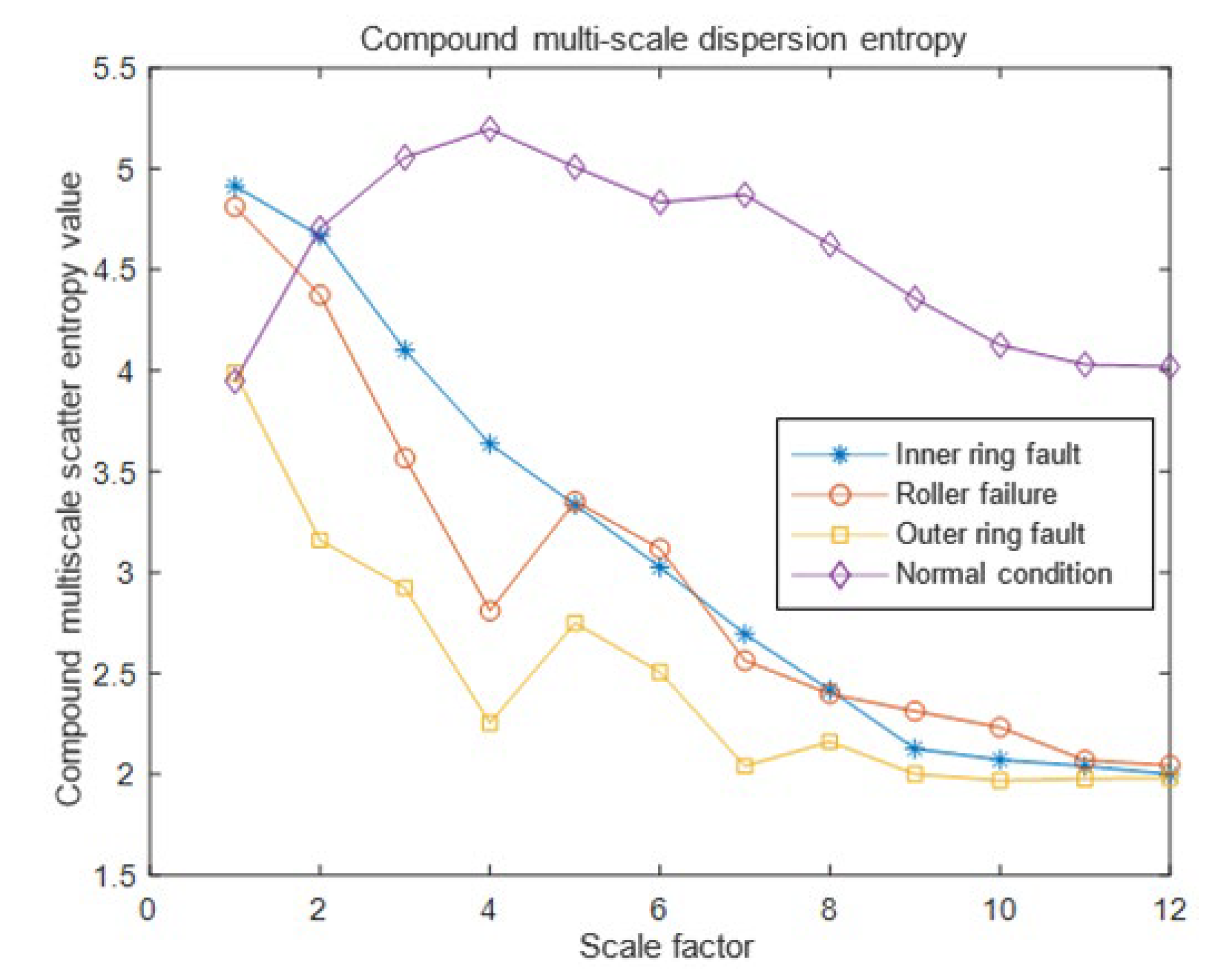
5. The Result Discussion

A total of 70 sets of multi-scale entropy eigenvalues of rolling bearing fault signals were substituted into the DBN model for recognition training. The DBN model was tested with 30 groups of test set data. Through the test, the experimental results show that the recognition accuracy of multi-scale arrangement entropy and DBN is 78.33%, the recognition accuracy of multi-scale dispersion entropy and DBN is 83.33%, and the recognition accuracy of composite multi-scale dispersion entropy and DBN is 90.33%. Each model is not particularly ideal in roller fault recognition. The experimental results show that the recognition accuracy of multi-scale arrangement entropy and optimized DBN is 98.33%, the recognition accuracy of multi-scale dispersion entropy and optimized DBN is 98.33%, and the recognition accuracy of composite multi-scale dispersion entropy and optimized DBN is 100%. Compared vertically, the PSO-DBN classification effect of the DBN model after optimizing parameters by the particle swarm optimization algorithm has been improved in different multi-scale entropy. Compared horizontally, the classification effect of the PSO-DBN model with different multi-scale entropy eigenvectors as input has also been significantly improved. Especially in the identification of roller fault, the three models have been greatly improved.

Through theoretical proof and experimental verification, the combination of VMD, CMDE, DBN, and PSO algorithm is very effective in rolling bearing fault diagnosis and identification. The main conclusions are as follows:

The rolling bearing fault recognition model is established; the eigenvectors are substituted into the DBN and PSO-DBN models, trained and tested; and the final experimental results are obtained. By comparing the recognition accuracy of DBN and PSO-DBN, it can be concluded that the PSO-DBN model has a higher recognition rate than the DBN model. Overall, the recognition rate based on VMD-CMDE-PSO-DBN is the best, which provides new insight for signal pattern recognition.

6. Conclusions

In this paper, an intelligent fault diagnosis method based on Variational Mode Decomposition (VMD), Composite Multi-scale Dispersion Entropy (CMDE), and Deep Belief Network (DBN) with Particle Swarm Optimization (PSO) algorithm—namely VMD-CMDE-PSO-DBN—is proposed. The decomposed number of modal components of VMD is determined by the observation center frequency, reconstructed according to the kurtosis, and the composite multi-scale dispersion entropy of the reconstructed signal is calculated to form the training samples and test samples of pattern recognition.

• The experimental data used in this paper are manually added faults, which may not fully reflect the diversified faults of rolling bearings, single fault forms, and low bearing speed. Under actual working conditions, bearings are mostly in high-speed operation and the fault forms are complex, so the next step should be to focus on the high-speed operation of rolling bearings and the composite fault state.
• VMD multi-scale permutation entropy eigenvector, VMD multi-scale dispersion entropy eigenvector, and VMD composite multi-scale dispersion entropy eigenvector is used as the inputs of the Deep Belief Network classification model. The accuracy of VMD decomposition composite multi-scale dispersion entropy is the best.

References

1. He, Z.; Shao, H.; Wang, P.; Lin, J.; Cheng, J. Deep transfer multi-wavelet auto-encoder for intelligent fault diagnosis of gearbox with few target training samples. Knowl. Based Syst. 2020, 191, 105313. [Google Scholar] [CrossRef]
2. Li, X.; Zhao, H.; Yu, L.; Chen, H.; Deng, W.; Deng, W. Feature extraction using parameterized multisynchrosqueezing transform. IEEE Sens. J. 2022, 2, 14263–14272. [Google Scholar] [CrossRef]
3. Xu, G.; Bai, H.; Xing, J.; Luo, T.; Xiong, N.N. SG-PBFT: A secure and highly efficient distributed blockchain PBFT consensus algorithm for intelligent Internet of vehicles. J. Parallel Distrib. Comput. 2022, 164, 1–11. [Google Scholar] [CrossRef]
4. Zheng, J.J.; Yuan, Y.; Zou, L.; Deng, W.; Guo, C.; Zhao, H. Study on a novel fault diagnosis method based on VMD and BLM. Symmetry 2019, 11, 747. [Google Scholar] [CrossRef]
5. Wu, D.; Wu, C. Research on the Time-Dependent Split Delivery Green Vehicle Routing Problem for Fresh Agricultural Products with Multiple Time Windows. Agriculture 2022, 12, 793. [Google Scholar] [CrossRef]
6. Zhou, X.B.; Ma, H.J.; Gu, J.G.; Chen, H.L.; Deng, W. Parameter adaptation-based ant colony optimization with dynamic hybrid mechanism. Eng. Appl. Artif. Intell. 2022, 114, 105139. [Google Scholar] [CrossRef]
7. Wu, X.; Wang, Z.C.; Wu, T.H.; Bao, X.G. Solving the family traveling salesperson problem in the adleman–lipton model based on DNA computing. IEEE Trans. NanoBioscience 2021, 21, 75–85. [Google Scholar] [CrossRef]
8. Li, X.; Shao, H.; Lu, S.; Xiang, J.; Cai, B. Highly-efficient fault diagnosis of rotating machinery under time-varying speeds using LSISMM and small infrared thermal images. IEEE Trans. Syst. Man Cybern. Syst. 2022, 50, 1–13. [Google Scholar] [CrossRef]
9. An, Z.; Wang, X.; Li, B.; Xiang, Z.L.; Zhang, B. Robust visual tracking for UAVs with dynamic feature weight selection. Appl. Intell. 2022. [Google Scholar] [CrossRef]
10. Cao, H.; Shao, H.; Zhong, X.; Deng, Q.; Yang, X.; Xuan, J. Unsupervised domain-share CNN for machine fault transfer diagnosis from steady speeds to time-varying speeds. J. Manuf. Syst. 2022, 62, 186–198. [Google Scholar] [CrossRef]
11. Li, T.Y.; Shi, J.Y.; Deng, W.; Hu, Z.D. Pyramid particle swarm optimization with novel strategies of competition and cooperation. Appl. Soft Comput. 2022, 121, 108731. [Google Scholar] [CrossRef]
12. Deng, W.; Xu, J.; Gao, X.; Zhao, H. An enhanced MSIQDE algorithm with novel multiple strategies for global optimization problems. IEEE Trans. Syst. Man Cybern. Syst. 2022, 52, 1578–1587. [Google Scholar] [CrossRef]
13. Chen, H.Y.; Miao, F.; Chen, Y.J.; Xiong, Y.J.; Chen, T. A hyperspectral image classification method using multifeature vectors and optimized KELM. IEEE J. Sel. Top. Appl. Earth Obs. Remote Sens. 2021, 14, 2781–2795. [Google Scholar] [CrossRef]
14. Yao, R.; Guo, C.; Deng, W.; Zhao, H.M. A novel mathematical morphology spectrum entropy based on scale-adaptive techniques. ISA Trans. 2022, 126, 691–702. [Google Scholar] [CrossRef]
15. Deng, W.; Li, Z.; Li, X.; Chen, H.; Zhao, H. Compound fault diagnosis using optimized MCKD and sparse representation for rolling bearings. IEEE Trans. Instrum. Meas. 2022, 71, 3508509. [Google Scholar] [CrossRef]
16. Tian, C.; Jin, T.; Yang, X.; Liu, Q. Reliability analysis of the uncertain heat conduction model. Comput. Math. Appl. 2022, 119, 131–140. [Google Scholar] [CrossRef]
17. Zhao, H.M.; Liu, J.; Chen, H.Y.; Chen, J.; Li, Y.; Xu, J.J.; Deng, W. Intelligent diagnosis using continuous wavelet transform and gauss convolutional deep belief network. IEEE Trans. Reliab. 2022, 1–11. [Google Scholar] [CrossRef]
18. Zhou, Y.; Zhang, J.; Yang, X.; Ling, Y. Optimal reactive power dispatch using water wave optimization algorithm. Oper. Res. 2020, 20, 2537–2553. [Google Scholar] [CrossRef]
19. Cui, H.; Guan, Y.; Chen, H. Rolling element fault diagnosis based on VMD and sensitivity MCKD. IEEE Access 2021, 9, 120297–120308. [Google Scholar] [CrossRef]
20. Xu, Y.; Chen, H.; Luo, J.; Zhang, Q.; Jiao, S.; Zhang, X. Enhanced Moth-flame optimizer with mutation strategy for global optimization. Inf. Sci. 2019, 492, 181–203. [Google Scholar] [CrossRef]
21. Liu, Q.; Jin, T.; Zhu, M.; Tian, C.; Li, F.; Jiang, D. Uncertain currency option pricing based on the fractional differential equation in the Caputo sense. Fractal Fract. 2022, 6, 407. [Google Scholar] [CrossRef]
22. Li, G.; Li, Y.; Chen, H.; Deng, W. Fractional-order controller for course-keeping of underactuated surface vessels based on frequency domain specification and improved particle swarm optimization algorithm. Appl. Sci. 2022, 12, 3139. [Google Scholar] [CrossRef]
23. Wei, Y.Y.; Zhou, Y.Q.; Luo, Q.F.; Deng, W. Optimal reactive power dispatch using an improved slime Mould algorithm. Energy Rep. 2021, 7, 8742–8759. [Google Scholar] [CrossRef]
24. Jin, T.; Xia, H.; Deng, W.; Li, Y.; Chen, H. Uncertain fractional-order multi-objective optimization based on reliability analysis and application to fractional-order circuit with Caputo type. Circ. Syst. Signal Pract. 2021, 40, 5955–5982. [Google Scholar] [CrossRef]
25. Xu, G.; Dong, W.; Xing, J.; Lei, W.; Liu, J. Delay-CJ: A novel cryptojacking covert attack method based on delayed strategy and its detection. Digit. Commun. Netw. 2022. [Google Scholar] [CrossRef]
26. Wu, E.Q.; Zhou, M.; Hu, D.; Zhu, L.; Tang, Z. Self-paced dynamic infinite mixture model for fatigue evaluation of pilots’ brains. IEEE Trans. Cybern. 2022, 52, 5623–5638. [Google Scholar] [CrossRef]
27. Jiang, M.; Yang, H. Secure outsourcing algorithm of BTC feature extraction in cloud computing. IEEE Access 2020, 8, 106958–106967. [Google Scholar] [CrossRef]
28. Deng, W.; Ni, H.C.; Liu, Y.; Chen, H.L.; Zhao, H.M. An adaptive differential evolution algorithm based on belief space and generalized opposition-based learning for resource allocation. Appl. Soft Comput. 2022. [Google Scholar] [CrossRef]
29. Zosso, D.; Dragomiretskiy, K. Variational mode decomposition. In IEEE Transactions on Signal Processing: A Publication of the IEEE Signal Processing Society; IEEE: Piscataway, NJ, USA, 2014. [Google Scholar]
30. Rostaghi, M.; Azami, H. Dispersion Entropy: A measure for time series analysis. IEEE Signal Process. Lett. 2016, 23, 610–614. [Google Scholar] [CrossRef]
31. Zhang, S.; Sun, G.; Li, L.; Li, X.; Jian, X. Study on mechanical fault diagnosis method based on LMD approximate entropy and fuzzy C-means clustering. Chin. J. Sci. Instrum. 2013, 34, 714–720. [Google Scholar]
32. Wang, J.; Shuai, C.; Chao, Z. Fault diagnosis method of gear based on VMD and multi-feature fusion. J. Mech. Transm. 2017, 3, 032. [Google Scholar]
33. Li, C. Research on Rolling Bearing Fault Diagnosis Method Based on Empirical Wavelet Transform and Scattered Entropy; Anhui University of Technology: Anhui, China, 2019. [Google Scholar]
34. Hinton, G.; Osindero, S.; Teh, Y. A fast learning algorithm for deep belief nets. Neura I Comput. 2006, 18, 1527–1554. [Google Scholar] [CrossRef] [PubMed]
35. Lei, Y.; Jia, F.; Zhou, X.; Lin, J. A Deep learning-based method for machinery health monitoring with big data. J. Mech. Eng. 2015, 51, 49–56. [Google Scholar] [CrossRef]
36. Li, W.; Shan, W.; Xu, Z.; Zeng, X. Bearing fault classification and recognition based on deep belief network. J. Vib. Eng. 2015, 29, 152–159. [Google Scholar]
37. Shi, P.; Liang, K.; Zhao, N. Gear intelligent fault diagnosis based on deep learning feature extraction and particle swarm support vector machine state recognition. China Mech. Eng. 2017, 28, 1056–1061. [Google Scholar]
38. Wang, W.; Carr, M.; Xu, W.; Kobbacy, K. A model for residual life prediction based on Brownian motion with an adaptive drift. Microelectron. Reliab. 2010, 51, 285–293. [Google Scholar] [CrossRef]
39. Sun, L.; Tang, X.G.; Zhang, X.H. Study of gearbox residual life prediction based on stochastic filtering model. Mech. Transm. 2011, 35, 56–60. [Google Scholar]
40. Deng, W.; Liu, H.; Xu, J.; Zhao, H.; Song, Y. An improved quantum-inspired differential evolution algorithm for deep belief network. IEEE Trans. Instrum. Meas. 2020, 69, 7319–7327. [Google Scholar] [CrossRef]
41. Zhao, H.; Liu, H.; Xu, J.; Guo, C.; Deng, W. Research on a fault diagnosis method of rolling bearings using variation mode decomposition and deep belief network. J. Mech. Sci. Technol. 2019, 33, 4165–4172. [Google Scholar] [CrossRef]
42. Li, T.; Qian, Z.; Deng, W.; Zhang, D.; Lu, H.; Wang, S. Forecasting crude oil prices based on variational mode decomposition and random sparse Bayesian learning. Appl. Soft Comput. 2021, 113PB, 108032. [Google Scholar] [CrossRef]
43. Pan, Y.; Chen, J.; Guo, L. Robust bearing performance degradation assessment method based on improved wavelet packet–support vector data description. Mech. Syst. Signal. Process. 2009, 23, 669–681. [Google Scholar] [CrossRef]
44. Dong, S.; Luo, T. Bearing degradation process prediction based on the PCA and optimized LS-SVM model. Measurement 2013, 46, 3143–3152. [Google Scholar] [CrossRef]
45. Xue, X.H. Evaluation of concrete compressive strength based on an improved PSO-LSSVM model. Comput. Concr. Int. J. 2018, 21, 505–511. [Google Scholar]
46. He, Q. Vibration signal classification by wavelet packet energy flow manifold learning. J. Sound Vib. 2013, 332, 1881–1894. [Google Scholar] [CrossRef]
47. Ishaque, K.; Salam, Z.; Amjad, M.; Mekhilef, S. An improved particle swarm optimization (PSO)–Based MPPT for PV with reduced steady-state oscillation. IEEE Trans. Power Electron. 2012, 27, 3627–3638. [Google Scholar] [CrossRef]
48. Roux, N.L.; Bengio, Y. Representational Power of Restricted Boltzmann Machines and Deep Belief Networks. Neural Comput. 2008, 20, 1631–1649. [Google Scholar] [CrossRef]
49. Larochelle, H.; Bengio, Y.; Louradour, J.; Lamblin, P. Exploring Strategies for Training Deep Neural Networks. J. Mach. Learn. Res. 2009, 1, 1–40. [Google Scholar]
Figure 1. Center frequency of the modal component K = 4.
Electronics 11 02582 g001
Figure 2. Center frequency of the modal component K = 5.
Electronics 11 02582 g002
Figure 3. Center frequency of the modal component K = 6.
Electronics 11 02582 g003
Figure 4. VMD-CMDE at τ = 8.
Electronics 11 02582 g004
Figure 5. VMD-CMDE at τ = 10.
Electronics 11 02582 g005
Figure 6. VMD-CMDE at τ = 12.
Electronics 11 02582 g006
Figure 7. DBN model.
Electronics 11 02582 g007
Figure 8. General flow chart of PSO-optimized DBN model.
Electronics 11 02582 g008
Figure 9. VMD-CMDE-DBN fault recognition rate.
Electronics 11 02582 g009
Figure 10. VMD-CMDE-PSO-DBN fault recognition rate.
Electronics 11 02582 g010