Article

A Modified LZW Algorithm Based on a Character String Parallel Search in Cluster-Based Telemetry Data Compression

School of Information and Electronics, Beijing Institute of Technology, Beijing 100081, China
*
Author to whom correspondence should be addressed.
Electronics 2022, 11(17), 2656; https://doi.org/10.3390/electronics11172656
Submission received: 29 June 2022 / Revised: 19 August 2022 / Accepted: 22 August 2022 / Published: 25 August 2022
(This article belongs to the Section Computer Science & Engineering)

Abstract

:
The volume of telemetry data is gradually increasing, both because of the increasingly larger number of parameters involved, and the use of higher sampling frequencies. Efficient data compression schemes are therefore needed in space telemetry systems to improve transmission efficiency and reduce the burden of required spacecraft resources, in particular regarding their transmitter power. In our primary study, a D-CLU algorithm was proposed to perform lossless compression for telemetry data, and achieve better performance. However, a limitation of this algorithm is that the compression time may become longer when the clustering head (CH) and outlier (which are compressed by LZW algorithm) numbers increase. To reduce compression delay, this paper proposed a modified character string (MCS) parallel search strategy for LZW algorithm (denoted by MCS-based LZW). The proposed MCS-based LZW algorithm designs coding principle, dictionary update rule and search strategy according to the character string matching results. Example verification and simulation results show that the proposed algorithm can effectively decrease the dictionary search times, and thus reduce the compression time.

1. Introduction

Aerospace telemetry data are the internal or external operating parameters of a spacecraft used to monitor and control the craft in orbit, and provide a basis for fault analysis and data processing [1]. In order to improve the transmission efficiency and reduce the spacecraft resource burden, particularly the transmitter power, efficient data compression is needed for space telemetry systems [2].
Several data compression algorithms are proposed for telemetry data, but suffer some problems for telemetry data compression, such as low compression ratio, high compression delay and error propagation [3,4,5,6]. To overcome these problems, a D-CLU algorithm is presented in [7]. This algorithm first proposes a clustering method based on the temporal–spatial correlation characteristic of telemetry data [8]; and then uses run-length encoding (RLE) and Lempel-Ziv-Welch (LZW) to perform data compression based on the clustering results. D-CLU algorithm can achieve better compression performance than other existing algorithms. However, there is one problem that should be further researched to improve telemetry data compression performance. In the D-CLU algorithm, LZW algorithm is used to perform intra-frame encode for clustering head (CH) and outlier frames. The compression delay of LZW algorithm is much larger than the RLE algorithm; thus, most of the compression delay of the D-CLU algorithm is generated by LZW algorithm. Therefore, when the CH and outlier number increases, the compression time of the D-CLU algorithm may become longer. It is necessary to research an improved LZW algorithm which can reduce the compression delay. Based on the above analyses, this study focuses on the further research of the LZW algorithm.
The compression time of the LZW algorithm is determined by dictionary size and searching strategy. Dictionary size can be set at an optimal value according to the real application. Thus, optimizing the searching strategy is a valuable idea to improve the performance of the LZW algorithm. The searching strategy for LZW can be classified into three categories: serial search, parallel search, and Hash-table search. Serial search strategy is a simple method which is easy to implement on a hardware platform, but with long search delay. Parallel search has shorter search delay than serial search, but with high control logic complexity. Hash-table search also has short search delay, but is not easy to implement on a hardware platform. Furthermore, Hash-table search has the problem of address ‘conflict’ [9]. To balance the search delay and complexity, a character-strings (CS)-based parallel method is proposed in [10]. This algorithm searches three character strings for matching with the dictionary at a time. It can reduce the search times at the beginning of the compression process. However, when the matching successful probability becomes higher, repeated searching for the character string may occur, leading to long compression delay. To overcome this problem, this paper proposes a modified CS-based parallel search strategy for the LZW algorithm (denoted by MCS-based LZW). The main contributions of this article are summarized as follows.
(1)
By analyzing data streaming clustering, the necessity for optimizing LZW algorithm is given. Inspired by the CluStream framework [11,12], a one-pass online clustering strategy is described in detail. In the cluster process, the CH and outlier number will be increased due to the abnormal data fluctuation. Thus, an improved LZW algorithm which can reduce compression time should be researched.
(2)
Analyze the limitation of CS-based parallel search strategy of LZW algorithm. The performance of this algorithm is better than serial search strategy and parallel search strategy [10]. However, the effectiveness of this algorithm is limited by the dictionary matching results.
(3)
An MCS-based LZW algorithm is proposed to reduce data compression time. An MCS-based LZW algorithm designs coding principle, dictionary update rule, and search strategy according to the character string matching results. This algorithm can effectively reduce dictionary search times and compression time.
The work is organized as follows: Section 2 briefly introduces the telemetry data characteristics and D-CLU algorithm; provides the detailed analysis of data streaming clustering. In Section 3, the limitation of CS-based search strategy is analyzed and the MCS-based parallel search strategy is proposed. The numerical results are provided in Section 4. Section 5 gives the conclusion part of this work.

2. Problem Formulation

In this section, the telemetry data characteristics and D-CLU compression algorithm are briefly introduced. Then, the necessity of optimizing LZW algorithm is given by analyzing the data streaming clustering.

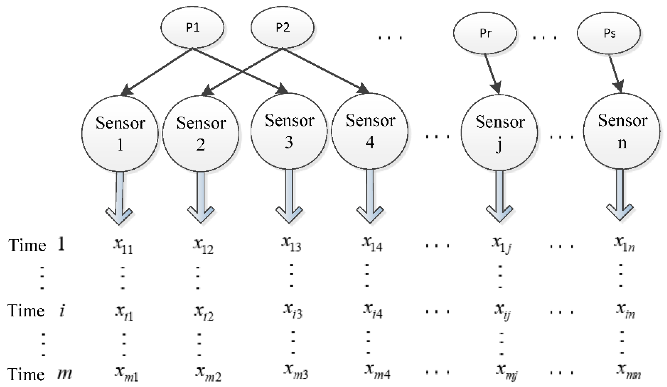
2.1. Telemetry Data Characteristics

The telemetry data are measurements from multiple parameters by multiple sensors, in which all parameters are sampled at the same rate. The Schematic diagram telemetry data acquisition is shown in Figure 1. The original data sampled over a certain period of time can be expressed as a telemetry matrix X m n which can be expressed as
X m × n = [ x 1 x i x m ] = [ x 11 x 1 j x 1 n x i 1 x i j x i n x m 1 x m j x m n ]     1 i m ,   1 j n
where, x i = { x i 1 , x i 2 , , x i j , , x i n } is the sample data collected at time i , and x i j denotes the j th element. As analyzed in [7], there are high levels of temporal correlation between neighboring rows of the telemetry matrix, and spatial correlation within the rows of the telemetry matrix. Temporal- spatial correlation is the basis of the D-CLU compression algorithm. Especially, temporal correlation makes it possible to group similar data into a cluster.

2.2. D-CLU Compression Algorithm

The telemetry matrix X m n = [ x 1 , , x i , , x m ] T can be considered as a real-time data streaming, and each row vector x i is considered as the basic element in the cluster. In the clustering process, some row vectors are determined as CHs, some row vectors are determined as cluster members (CMs), and others are determined as the outliers. Assume that x i and x c are two elements in a cluster, x i is a CM and x c is the CH, the difference between x i and x c can be expressed as
d i c = x i x c = { x i 1 x c 1 , , x i n x c n }
Based on the D-CLU compression algorithm, LZW is used to encode x i and outliers, and RLE is used to encode d i c . More detailed information about D-CLU compression algorithm is given in [7].

2.3. Analysis of Data Streaming Clustering Algorithm and the Problem Formulation

Data clustering partitions a data set into clusters according to certain similarity indices [13]. Several existing clustering methods are investigated in [14]. Aerospace telemetry data can be considered as data streaming, and it is thus suitable to use a data streaming clustering algorithm for data partition [15]. CluStream is a classical data streaming clustering framework; based on this framework, the data streaming clustering is typically done as a two-stage process with an online part which summarizes the data into many micro-clusters, and then, in an offline process, these micro-clusters are merged into a smaller number of final clusters [16]. Inspired by the online cluster idea of CluStream framework, one-pass data streaming clustering strategy is used in the D-CLU algorithm.
Data streaming clustering is process whereby new clusters continue to emerge and old clusters continue to disappear. As shown in Figure 2, the cluster which has been disappeared is defined as a past cluster, and the cluster which is now processing is defined as a current cluster.
For a new input x i , the cluster process is shown in Figure 3. It can be seen that the cluster process is to determine whether the new input belongs to the current cluster or not. Assume that x c is the CH of the current cluster, the similarity (denoted by S ( x i , x c ) between x i and x c is calculated and compared with a predefined threshold V h . If S ( x i , x c ) V h , the new input belongs to the current cluster as a new CM; otherwise, the new input is determined as a potential CH (P-CH) and the current cluster becomes a past cluster. For a P-CH, it may become a CH of a new cluster or an outlier.
The data streaming clustering process for a P-CH is shown in Figure 4. Let x c p denote the current P-CH, and the next new input is denoted by x i + 1 . The similarity between x i + 1 and x c p are calculated and compared with V h . If S ( x i + 1 , x c p ) V h , the current P-CH is determined as the CH of the new cluster, and x i + 1 is determined as the first CM of the new cluster; otherwise, the current P-CH is determined as a outlier, and x i + 1 is determined as a new P-CH.
Based on above analyses, the results of data streaming clustering are determined by the similarity. In application, if the telemetry data fluctuates abnormally over a period of time, the similarity between data stream elements will be reduced, leading to an increase in the CH and outlier number. CHs and outliers are compressed by LZW algorithm. Large CH and outlier numbers would increase the compression time cause by the code delay of the LZW algorithm. In order to overcome this problem, an improved LZW algorithm based on a modified CS parallel search strategy is proposed.

3. Methodology

3.1. Analyses of CS-Based LZW Algorithm

CS-based LZW algorithm searches three character strings at a time, and matches with the character strings which have been stored in the dictionary; then outputs codeword and updates the dictionary according to the matching results. Let a i denote a character. Let { a i , a j } denote a character string where a i and a j are the prefix and suffix of the character string, respectively. Let R c s denote the matching result. Three character strings are searched each time, thus 8 matching results may be obtained, i.e., { 000 } , { 001 } , { 010 } , { 011 } , { 100 } , { 101 } , { 110 } , { 111 } , where ‘0’ indicates a failed matching, and ‘1’ indicates a successful matching. The coding principle and dictionary update rules of CS-based LZW algorithm can be summarized in Table 1. Here, we assume that the current searching character strings are { a i , a i + 1 } , { a i + 1 , a i + 2 } , { a i + 2 , a i + 3 } , and the current dictionary address maximum index is M . ( M + 1 ) = { a i , a i + 1 } denotes that the address index of { a i , a i + 1 } in the dictionary is M + 1 ; O denotes the output codeword; P s _ n e x t denotes the prefix of the first character string that corresponding to the next searching process; d ( { a i , a i + 1 } ) denotes the address index of { a i , a i + 1 } stored in the dictionary.
The limitation of CS-based LZW algorithm is that a repeated search may occur for a character string when the matching successful probability is high, which is considered to increase the searching time. To illustrate this problem, an example is discussed here. Assume that the input character sequence is { a 1 , a 2 , a 3 , a 4 , a 2 , a 3 , a 5 , a 6 , a 7 , } . The current searching character strings are { a 1 , a 2 } , { a 2 , a 3 } and { a 3 , a 4 } , and they have been stored in the dictionary, i.e., ( 256 ) = { a 1 , a 2 } , ( 257 ) = { a 2 , a 3 } and ( 258 ) = { a 3 , a 4 } . Thus, the current matching result is { 111 } . For simplicity, the current search stage is denoted by S1, and the next search stage is S2. Based on the coding principle and dictionary update rules stated in Table 1, the search process can be illustrated in Figure 5. At the stage of S1, the matching result is { 111 } ; there is no output codeword and dictionary update, and P s _ n e x t is address index of { a 1 , a 2 } . Thus, at the stage of S2, the second sets of character strings that to be searched are { 256 , a 3 } , { a 3 , a 4 } and { a 4 , a 2 } ; the matching result is { 010 } , dictionary update can be denoted by ( 259 ) = { 256 , a 3 } , the output codeword is 256, and P s _ n e x t is the address index of { a 3 , a 4 } , i.e., 258. Thus, at the stage of S3, the third sets of character strings that to be searched are { 258 , a 2 } , { a 2 , a 3 } and { a 3 , a 5 } ; the matching result is { 010 } , dictionary update can be denoted by ( 260 ) = { 258 , a 2 } , the output codeword is 258, and P s _ n e x t is the address index of { a 2 , a 3 } , i.e., 257. From this example, for the character stings { a 1 , a 2 } , { a 2 , a 3 } and { a 3 , a 4 } need to be searched three times (S1 to S3) to complete the coding. { a 3 , a 4 } is searched two times (S1 and S2), i.e., a repeated search occurred for { a 3 , a 4 } .
Based on the above analyses, when the matching successful probability is high, the CS-based algorithm cannot reduce the dictionary search times. To solve this problem, we proposed an MCS-based LZW algorithm to reduce dictionary searching times.

3.2. MCS-Based LZW Algorithm

Let R = { R 1 R 2 R i R i + 1 R i + 2 R N } denote the matching result of character-strings parallel search at a time, where R i is the matching result of the i th character string; N is the number of character string in each parallel search process. The main idea of the proposed MCS-based LZW algorithm is to directly give the output codeword and dictionary update rules according to the matching result. The design of the MCS-based LZW algorithm contains of three parts: coding principle, dictionary update rules and selection of P s _ n e x t .

3.2.1. Coding Principle

Let O = { O 1 , O 2 , , O i , O i + 1 , O N } denote the output codeword corresponding to R ; let C ( R i ) denote the character string corresponding to R i ; let A ( R i ) denote the address index of C ( R i ) if C ( R i ) has been already stored in the dictionary; let P ( R i ) denote the prefix of C ( R i ) . If R i is selected to determine the output codeword, O i can be obtained by
O i = { A ( R i ) , R i = 1 P ( R i ) , R i = 0
However, if R i is not selected to determine O i , O i is null. One situation would cause R i not to be selected, i.e., R i 1 is selected and R i 1 = 1 .
Let us provide an example to illustrate the coding principle. Assume that the matching result is R = { R 1 R 2 R 3 R 4 } = { 1001 } , A ( R 1 ) and A ( R 4 ) are M 1 and M 4 , respectively. It can be seen that R 1 = 1 , according to (3), O 1 is M 1 . Because that R 1 is selected and R 1 = 1 , thus O 2 is null. It can be seen that R 3 = 0 , thus O 3 is P ( R 3 ) . Similarly, we can obtain O 4 is M 4 . Finally, the output codeword for R = { 1001 } is O = { M 1 , P ( R 3 ) , M 4 } .

3.2.2. Dictionary Update Rules

Let D = { D 1 , D 2 , , D i , D i + 1 , D N } denote the dictionary update result corresponding to R . If R i is selected to determine D i , the dictionary update rules can be expressed as
D i ( d ) = { no update , R i = 1 C ( R i ) , R i = 0
where, d is the address index in the dictionary. If R i is not selected to determine D i , the dictionary update is null (denoted by no update).
We also take R = { R 1 R 2 R 3 R 4 } = { 1001 } as an example to illustrate the dictionary update rules. It can be seen that R 1 = 1 ; thus, the dictionary is not updated (denoted by no update). Because that R 1 is selected and R 1 = 1 , D 2 ( d ) is null. It can be seen that R 3 = 0 , thus D 3 ( d ) is C ( R 3 ) . Similarly, D 4 ( d ) is determined by R 4 , i.e., D 4 ( d ) = C ( R 4 ) . Finally, the dictionary update result for R = { 1001 } is D = { C ( R 3 ) , C ( R 4 ) } .
Based on above descriptions, the flowchart of the coding principle and dictionary update rules can be summarized in Figure 6.

3.2.3. Selection of P s _ n e x t

In the MCS-based LZW algorithm, P s _ n e x t is determined by the value of R N ; two cases may be occurred. When R N = 1 and R N is selected to generate O N and D N , P s _ n e x t is the new input character; otherwise, P s _ n e x t is the suffix of C ( R N ) . When, P s _ n e x t is the suffix of C ( R N ) . In summary, P s _ n e x t can be expressed as
P s _ n e x t = { suffix   of C ( R N ) , R N = 1 a n d R N 1 = 1 a n d R N 1 i s s e l e c t e d new   input   character , R N = 1 a n d R N 1 = 1 a n d R N 1 i s n o t s e l e c t e d new   input   character , R N = 1 a n d R N 1 = 0 suffix   of C ( R N ) , R N = 0
We take R = { R 1 R 2 R 3 R 4 } = { 1001 } as an example again. It can be seen that R N = 1 and R N 1 = 0 , thus P s _ n e x t is the new input character.
To compare to the CS-based LZW algorithm, we provide the coding principle and dictionary update of the MCS-based LZW algorithm at N = 3 , which are shown in Table 2. Assume that the current searching character strings are { a i , a i + 1 } , { a i + 1 , a i + 2 } , { a i + 2 , a i + 3 } and the current dictionary address maximum index is M . It can be seen that when the matching results are { 100 } , { 101 } , { 110 } and { 111 } , MCS-based LZW algorithm outputs the codeword, but CS-based LZW algorithm has no output codeword. This shows that the CS-based LZW algorithm needs a further dictionary search for coding these character strings. In particular, when R = { 111 } , the MCS-based LZW algorithm only searches the dictionary one time to complete encoding, but the CS-based LZW algorithm needs to search three times, as can be seen in Figure 5.

3.2.4. Complexity Analyses

The computational complexity of LZW algorithm can be calculated as
T = T d i c _ o n e N s e a r c h
where T d i c _ o n e is the computational complexity of one dictionary search, and N s e a r c h is the dictionary search time. For different LZW algorithms, T d i c _ o n e is the same under the same initial condition. Thus, the computational complexity is determined by the value of N s e a r c h . It can be seen that reducing dictionary search times could decrease the computational complexity. In the MCS-based algorithm, the value of N s e a r c h can be calculated by
N s e a r c h = N s e q / 3
where, N s e q is the number of characters in the input sequence. In the CS-based LZW algorithm, when the successful probability of dictionary matching result becomes higher, repeated search process occurs as described in Figure 5. However, the MCS-based algorithm can avoid repeated search. Thus, the value of N s e a r c h obtained by MCS-based LZW is lower than CS-based LZW algorithm. Therefore, the computational complexity of MCS-based LZW is lower than the CS-based LZW algorithm. In theory, decreasing the computational complexity could decrease the compression time; thus, the compression time of the MCS-based LZW algorithm would be lower than that of the CS-based LZW algorithm.

4. Implementations

This section will provide an example and several MATLAB implementations to verify the performance of proposed MCS-based LZW algorithm.

4.1. Example Verification

The performance of MCS-based LZW algorithm is verified through a group of randomly selected input sequences. The input sequence is {23,25,34,45,56,85,23,25,34,45,56,85,22,26,28,85,22,26,28,30,34}, set N = 3 and M = 255. The coding and decoding processes are shown in Table 3 and Table 4, respectively. By decoding, the output sequence is the same as the input sequence, which proves the effectiveness of MCS-based LZW algorithm. As can be seen form Table 3, only by 7 searching times are needed for 21 characters encoding when using MCS-based LZW algorithm; however, 13 searching times and 21 searching times are needed when using CS-based LZW algorithm and conventional LZW algorithm, respectively. As analyzed in Section 3.2.4, the MCS-based LZW algorithm has the lowest computational complexity. Therefore, the proposed MCS-based LZW algorithm can reduce compression time compared with other LZW algorithms.

4.2. MATLAB Implementations

In order to verify the performance of the MCS-based LZW algorithm, MATLAB software package was utilized to implement the algorithm. The evaluations were performed using 12 real-world datasets (D-1 to D-12) from a certain aerospace application, where 6 datasets (D-1 to D-6) were the same as [7]. For each dataset, the telemetry data matric contains 2000 rows of 512 bytes, for a total of 1024 KB. We have selected the space saving (SS) and compression time (CT) to verify the performance of the LZW algorithm. SS is defined as
S S = ( 1 z / z ) × 100 %
where z and z are the uncompressed size and compressed size, respectively.
In this section, SS comparisons for three LZW algorithms are firstly provided. Then the compression ratio of the D-CLU algorithm by using LZW compression and without using LZW compression are given. Finally, the compression time of the D-CLU algorithm by using LZW compression and without using LZW compression are provided.
Table 5 shows the SS comparisons for three LZW algorithms. For each dataset, LZW algorithm is applied for each data frame to obtain the space savings, and then calculating an average value. It can be seen that the SS of MCS-based LZW algorithm has not been improved greatly compared with other two existing LZW algorithms. Three algorithms have a similar performance in terms of SS.
Figure 7 shows the CT comparisons for three LZW algorithms. For each dataset, LZW algorithm is applied for each data frame to obtain the CTs, and then calculating an average value. It can be seen that the MCS-based LZW algorithm has a lower compression time than the other two LZW algorithms.
Table 6 shows the SS comparisons for D-CLU algorithm by using conventional LZW, CS-based LZW and MCS-based LZW, respectively. In addition, in order to further verify the influence of LZW algorithm on D-CLU algorithm, the compression rate of D-CLU algorithm without using LZW compression is also added to make comparisons. It can be seen that the SSs of D-CLU algorithm by using LZW compression are similar, and higher than that without using LZW compression.
Figure 8 shows the CTs of D-CLU algorithm by using conventional LZW, CS-based LZW, MCS-based LZW, and without using LZW compression, respectively. For each simulation, the CT is obtained by the functions “tic” and “toc” of MATLAB. For each dataset, 500 times simulations are performed and calculated an average value. It can be seen that the D-CLU algorithm without using LZW compression has the lowest CTs. This is because the compression delay of the LZW algorithm is higher than that of the RLE algorithm. Without using LZW compression, the CTs of D-CLU are mainly determined by RLE compression. By using LZW compression, the CTs of D-CLU algorithm clearly become higher. By comparison, the CTs of D-CLU algorithm by using MCS-based LZW are lower than by using conventional LZW and CS-based LZW. This is because that MCS-based LZW algorithm could use less time for a dictionary search which is considered to decrease the compression delay. From these simulation results, the proposed MCS-based LZW algorithm could reduce compression time while ensuring the similar space savings compared with the existing LZW algorithms.

5. Conclusions

This work presented an MCS-based LZW algorithm which is used for aerospace telemetry data compression. D-CLU compression algorithm was briefly introduced, and the data streaming clustering algorithm was analyzed to give the necessity of optimizing the LZW algorithm. The limitation of the CS-based parallel search strategy was analyzed and the MCS-based LZW algorithm was proposed. The proposed algorithm outputs the codeword and updates the dictionary according to the matching result between the current searching character strings and character strings stored in the dictionary. The coding principle and dictionary update rules were provided. An example verification showed that the improved LZW can reduce the search times compared with other LZW algorithms. To further verify the performance of the improved LZW algorithm, simulations were performed for the D-CLU algorithm using different LZW algorithms and without using the LZW algorithm. Compared to without using LZW algorithm, the D-CLU algorithm by using MCS-based LZW algorithm can obtain a 5-percentage-point space saving at the expense of increasing compression delay (factor 2–3). Compared to other existing LZW algorithms, the D-CLU algorithm by using MCS-based LZW algorithm can reduce the compression time while ensuring similar space savings. Although the proposed modified LZW algorithm is presented on the basis of the D-CLU compression algorithm, it can also be used in other fields that need to perform data compression by using the LZW algorithm. Therefore, the proposed method is valuable in data compression fields.

Author Contributions

Conceptualization, X.S. and Y.H.; Methodology, X.S. and Y.H.; Software, X.S.; Formal Analysis, Y.H.; Investigation, Y.W.; Resources, Y.W.; Data Curation, Y.H.; Writing—Original Draft Preparation, X.S.; Writing—Review & Editing, X.S.; Funding Acquisition, X.S. All authors have read and agreed to the published version of the manuscript.

Funding

This research was funded by National Natural Science Foundation grant number 62101047, and China Postdoctoral Science Foundation grant number 2020TQ0044.

Conflicts of Interest

The authors declare no conflict of interest.

References

  1. Giannini, A.; Pelorossi, F.; Pasian, M.; Bozzi, M.; Perregrini, L.; Besso, P.; Garramone, L. The Sardinia Radio Telescope Upgrade to Telemetry, Tracking and Command: Beam Squint and Electromagnetic Compatibility Design. IEEE Antennas Propag. Mag. 2015, 57, 177–191. [Google Scholar] [CrossRef]
  2. Wang, Q.; Wang, B.; Wu, B. Study on Threats to Security of Space TT&C Systems. In Proceedings of the 26th Conference of Spacecraft TT&C Technology in China; Springer: Berlin/Heidelberg, Germany, 2013; pp. 67–73. [Google Scholar]
  3. Beglaryan, G. Lossless Compression of Aerospace Telemetry Data for a Narrow-Band Downlink. Ph.D. Thesis, California State University, Northridge, CA, USA, 2014. [Google Scholar]
  4. Abraham, J.G.; Mishra, R.; Deepa, J. A lossless compression algorithm for vibration data of space systems. In Proceedings of the International Conference on Next Generation Intelligent Systems, Kottayam, India, 1–3 September 2016; pp. 1–7. [Google Scholar]
  5. CCSDS 121.0-B-2; CCSDS, Lossless Data Compression. Recommendation for Space Data Systems Standards. Blue Book: Washington, DC, USA, May 2012.
  6. Li, G.; Zhang, R.; Shi, J. Lossless data compression algorithm for aerospace packet telemetry data. In Proceedings of the 2013 International Conference on Mechatronic Sciences, Electric Engineering and Computer, Shenyang, China, 20–22 December 2013; pp. 2756–2759. [Google Scholar]
  7. Shi, X.; Shen, Y.; Wang, Y.; Bai, L. Differential-Clustering Compression Algorithm for Real-Time Aerospace Telemetry Data. IEEE Access 2019, 6, 57425–57433. [Google Scholar] [CrossRef]
  8. Ling, C.; Zou, L.J.; Tu, L. A clustering algorithm for multiple data streams based on spectral component similarity. Inf. Sci. 2012, 183, 35–47. [Google Scholar]
  9. Laarman, A.; Pol, J.; Weber, M. Parallel Recursive State Compression for Free. In International Spin Conference on Model Checking Software; Springer: Berlin/Heidelberg, Germany, 2017; pp. 38–56. [Google Scholar]
  10. Liu, M. Research and Implementation of Lossless Compression Technique for Space Telemetry Data. Master’s Thesis, Beijing Institute of Technology, Beijing, China, 2016; pp. 24–28. [Google Scholar]
  11. Sangam, R.S.; Om, H. Equi-clustream: A framework for clustering time evolving mixed data. Adv. Data Anal. Classif. 2018, 12, 973–995. [Google Scholar] [CrossRef]
  12. Sayed, D.; Rady, S.; Aref, M. Enhancing clustream algorithm for clustering big data streaming over sliding window. In Proceedings of the International Conference on Electrical Engineering, Cairo, Egypt, 7–9 July 2020; pp. 108–114. [Google Scholar]
  13. Solanki, S.K.; Patel, J.T. A Survey Paper on Parallel Power Iteration Clustering for Big Data. Intern. J. Innov. Res. Technol. 2014, 1, 1–5. [Google Scholar]
  14. Ibrahim, A.; Hassanien, R. Homogenous and Heterogenous Parallel Clustering: An Overview. arXiv 2022, arXiv:2202.06478. [Google Scholar]
  15. Xin, D.; Pi, D. An Effective Method for Mining Quantitative Association Rules with Clustering Partition in Satellite Telemetry Data. In Proceedings of the International Conference on Advanced Cloud and Big Data, Huangshan, China, 20–22 November 2014; pp. 26–33. [Google Scholar]
  16. Hahsler, M.; Bolaños, M. Clustering Data Streams Based on Shared Density between Micro-Clusters. IEEE Trans. Knowl. Data Eng. 2016, 28, 1449–1461. [Google Scholar] [CrossRef]
Figure 1. Schematic diagram of telemetry data acquisition.
Electronics 11 02656 g001
Figure 2. Clustering structure of data streaming clustering in D-CLU algorithm.
Electronics 11 02656 g002
Figure 3. Data streaming clustering process for a new input.
Electronics 11 02656 g003
Figure 4. Data streaming clustering process for a P-CH.
Electronics 11 02656 g004
Figure 5. Coding process of the CS-based LZW algorithm for R c s = { 111 } .
Electronics 11 02656 g005
Figure 6. Flowchart of the coding principle and dictionary update rules.
Electronics 11 02656 g006
Figure 7. CT comparisons of three LZW algorithms.
Electronics 11 02656 g007
Figure 8. CTs of the D-CLU algorithm by using LZW compression and without using LZW compression.
Electronics 11 02656 g008
Table 1. The coding principle and dictionary update of the CS-based LZW algorithm.
R c s Dictionary Update O P s _ n e x t
000 ( M + 1 ) = { a i , a i + 1 } , ( M + 2 ) = { a i + 1 , a i + 2 } , ( M + 3 ) = { a i + 2 , a i + 3 } a i , a i + 1 , a i + 2 a i + 3
001 ( M + 1 ) = { a i , a i + 1 } ( M + 2 ) = { a i + 1 , a i + 2 } a i , a i + 1 d ( { a i + 2 , a i + 3 } )
010 ( M + 1 ) = { a i , a i + 1 } a i d ( { a i + 1 , a i + 2 } )
011 ( M + 1 ) = { a i , a i + 1 } a i d ( { a i + 1 , a i + 2 } )
100No updateNo output d ( { a i , a i + 1 } )
101No updateNo output d ( { a i , a i + 1 } )
110No updateNo output d ( { a i , a i + 1 } )
111No updateNo output d ( { a i , a i + 1 } )
Table 2. Coding principle and dictionary update of the MCS-based LZW algorithm ( N = 3 ).
R Dictionary Update O P
000 ( M + 1 ) = { a i , a i + 1 } , ( M + 2 ) = { a i + 1 , a i + 2 } , ( M + 3 ) = { a i + 2 , a i + 3 } a i , a i + 1 , a i + 2 a i + 3
001 ( M + 1 ) = { a i , a i + 1 } ( M + 2 ) = { a i + 1 , a i + 2 } a i , a i + 1 , d ( { a i + 2 , a i + 3 } a i + 4
010 ( M + 1 ) = { a i , a i + 1 } , ( M + 3 ) = { a i + 2 , a i + 3 } a i , d ( { a i + 1 , a i + 2 } ) a i + 3
011 ( M + 1 ) = { a i , a i + 1 } a i , d ( { a i + 1 , a i + 2 } ) a i + 3
100 ( M + 3 ) = { a i + 2 , a i + 3 } d ( { a i , a i + 1 } ) , d ( { a i + 2 , a i + 3 } ) a i + 3
101No update d ( { a i , a i + 1 } ) , d ( { a i + 2 , a i + 3 } ) a i + 4
110 ( M + 3 ) = { a i + 2 , a i + 3 } d ( { a i , a i + 1 } ) a i + 3
111No update d ( { a i , a i + 1 } ) , d ( { a i + 2 , a i + 3 } ) a i + 4
Table 3. Coding process of the MCS-based LZW algorithm.
Searching CS R Dictionary O
{23,25}{25,34}{34,45}000(256) = {23,25}, (257) = {25,34}, (258) = {34,45}23, 25, 34
{45,56}{56,85}{85,23}000(259) = {45,56}, (260) = {56,85}, (261) = {85,23}45, 56, 85
{23,25}{25,34}{34,45}111No update256, 258
{56,85}{85,22}{22,26}100(262) = {22,26}260, 22
{26,28}{28,85}{85,22}000(263) = {26,28}, (264) = {28,85}, (265) = {85,22}26, 28, 85
{22,26}{26,28}{28,30}110(266) = {28,30}262, 28
{30,34}{34,-}{-,-}0--(267) = {30,34}30, 34, -
Table 4. Decoding process of the MCS-based LZW algorithm.
Input CSOutputDictionaryInput CSOutputDictionary
{23,25}23D(256) = {23,25}{22,26}22(262) = {22,26}
{25,34}25D(257) = {25,34}{26,28}26(263) = {26,28}
{34,45}34(258) = {34,45}{28,85}28(264) = {28,85}
{45,56}45D(259) = {45,56}{85,262}85(265) = {85,22}
{56,85}56D(260) = {56,85}{262,28}22,26No update
{85,256}85(261) = {85,23}{28,30}28(266) = {28,30}
{256,258}23,25No update{30,34}30(267) = {30,34}
{258,260}34,45No update{34,-}34--
{260,22}56,85No update------
Table 5. SS comparisons of three LZW algorithms (%).
D-1D-2D-3D-4D-5D-6D-7D-8D-9D-10D-11D-12
Conventional LZW28.4732.4629.5241.2430.1235.2832.1128.7633.1331.2629.1528.43
CS-based LZW29.4333.2430.1542.1332.7136.233.0929.0833.1431.2731.2429.05
MCS-based LZW29.3133.2431.0742.2533.0236.4333.4130.133.2532.1131.3530.16
Table 6. SSs of D-CLU algorithm by using LZW compression and without using LZW compression (%).
D-1D-2D-3D-4D-5D-6D-7D-8D-9D-10D-11D-12
No LZW45.3147.1645.7947.2146.9247.2442.1641.0243.1841.5440.8942.38
Conventional LZW50.2151.3449.0550.7648.3751.5446.845.944.745.245.146.3
CS-based LZW51.251.5249.5551.1748.1650.8446.9545.2545.1744.1645.1246.98
MCS-based LZW51.5151.5450.2351.9848.5351.6147.0846.1645.3845.5145.3147.03
Publisher’s Note: MDPI stays neutral with regard to jurisdictional claims in published maps and institutional affiliations.

