The UAV Path Coverage Algorithm Based on the Greedy Strategy and Ant Colony Optimization

Abstract

Today, the development of unmanned aerial vehicles (UAVs) has attracted significant attention in both civil and military fields due to their flight flexibility in complex and dangerous environments. However, due to energy constraints, UAVs can only finish a few tasks in a limited time. The problem of finding the best flight path while balancing the task completion time and the coverage rate needs to be resolved urgently. Therefore, this paper proposes a UAV path coverage algorithm base on the greedy strategy and ant colony optimization. Firstly, this paper introduces a secondary advantage judgment and optimizes it using an ant colony optimization algorithm to reach the goal of minimum time and maximum coverage. Simulations are performed for different numbers of mission points and UAVs, respectively. The results illustrate that the proposed algorithm achieves a 2.8% reduction in task completion time while achieving a 4.4% improvement in coverage rate compared to several previous works.

1. Introduction

Nowadays, Unmanned Aerial Vehicle (UAV) technologies are rapidly developing and gaining attention from countries worldwide due to their faster moving speed and wider deployment range, mainly due to freedom to move. With these advantages, UAVs have a wide range of applications in military and civilian use, such as reconnaissance [1], surveillance [2], cargo delivery [3], natural disaster prevention or rescue [4,5], etc. Unlike crewed vehicles, UAVs can take humans out of dull, dirty, dangerous missions. The UAV usually works unsupervised, which requires them to choose the best collision-free coverage path from the start to the destination.

For example, suppose a UAV needs to patrol and monitor a complex area. In that case, the UAV will fly from the base to the location of a possible disaster to collect in-formation and eventually return to the base and generate an early warning situational map of the area. Although UAVs can effectively reduce costs and increase flexibility in large-area surveillance work, it also leads to serious path planning and mission assign-ment problems. In some cases, the flight time is irrelevant to the importance of the mis-sion point. UAVs sometimes have to fly very long times to important mission points. Failure to balance these two aspects will seriously undermine the effectiveness of the work in the mission area [6]. Meanwhile, the inefficient use or waste of energy can also seriously affect the efficiency of UAVs.

Therefore, it is challenging to design path planning algorithms in energy constraints conditions. This challenge also requires flight time and important mission point coordi-nation. In this paper, the problem is considered the minimum time and maximum cov-erage (MTMC) problem, where a group of UAVs is dispatched to effectively patrol tar-gets in a large-scale surveillance area to achieve the maximum coverage in the minimum mission time [7]. The importance of the mission points is quantified as the weight values. The MTMC problem is NP-hard because it is an extension of the well-known Traveling Salesman Problem. No efficient algorithm has been found for this problem, and only its practical approximate optimum can be obtained.

The details of the contribution of this paper can be summarized as follows.

(1)

Optimize the greedy algorithm using secondary advantage mechanism to balance the flight time and the importance of mission points.

(2)

Optimize the flight path using the ant colony algorithm to reduce the UAV flight time.

The rest of this paper is organized as follows. The related work of the paper is shown in Section 2. The system model and the details of the path planning algorithm are pre-sented in Section 3. The simulation results of the algorithm in this paper are given in Section 4. The conclusion and the prospect of future work are presented in Section 5.

2. Related Work

The path planning is essential to improving the efficiency of UAVs in performing reconnaissance, surveillance, search, and other tasks while moving through the mission area [8]. Meanwhile, the path planning techniques are classified into two categories, global path planning and local path planning, based on the available workspace information.

Firstly, when the environmental conditions are completely known, a global path planning algorithm is executed, which can also be called offline path planning. The already well-known global planning algorithms include the A* algorithm [9], Dijkstra algorithm [10], Rapid-exploration Random Tree (RRT) [11], Genetic Algorithm (GA) [12], Particle Swarm Optimization (PSO) [13], Ant Colony optimization (ACO) [14], Grey Wolf Optimizer (GWO) [15], Bat algorithm [16], etc.

Recently, more researchers have optimized the global path planning algorithms. In [17], Chenguang Liu et al. study a path planning problem using an improved A* algorithm. The objective is to improve the economy of the planned paths while maximizing mobility constraints. It should be noted that A* may find invalid paths due to the grid [18]. In [19], Sheng Gao et al. introduce a negative feedback mechanism into the ant colony optimization algorithm. In [20], Chen et al. use an adaptive parameter S to modify the probability of crossover and variation during the genetic operation. The methods in [18,19] both make the algorithm converge faster to a certain extent. Since biological heuristics occupy a large amount of calculative space, such as the GA, the algorithm’s convergence speed is influenced by the initial path. A bad initial path will cost a longer computation time. In [21], Pehlivanoglu et al. optimize the initial population in the genetic algorithm by the ant colony optimization algorithm to accelerate the convergence of the whole algorithm. In [22], Chengzhi Qu et al. optimize the grey wolf algorithm using a symbiotic biological search algorithm. To deal with the bat algorithm shortcoming that tends to fall into local optima, Xianjin Zhou et al. [23] optimize the bat algorithm using an artificial bee colony algorithm to improve the local search ability of the bat algorithm in a 3D environment.

Secondly, the local path planning or the online planning are referred to the research models in which the environmental information is completely unknown or partially known. The local planning algorithms usually include Artificial Potential Field (APF) method [24] and Dynamic Window Approach (DWA) [25], etc.

Recently, the local path planning has been continuously optimized by researchers [26]. Among them, the artificial potential field (APF) method has been widely used in UAV local path planning for its simplicity, efficiency, and path smoothing advantages. In [27], Song Jia et al. used the method of potential field prediction to solve the drawback that APFs easily fall into the local optima problem. With learning-based methods are widely used [28]. In [29,30,31], methods such as YOLOv4-CSP, Q-learning and Deep Reinforcement Learning are used to improve the speed and accuracy of the algorithms. However, the algorithm cannot resolve whether the flight path follows the original global path planning method or performs local path planning first and then replans.

Perferct global path planning is particularly important for long-range navigation in large-scale mission areas due to the battery life limitation. In the application scenario of this paper, the task completion time and coverage rate are the key performance indicators [7,32].

In [33], Cho et al. propose a grid-based area decomposition method that uses UAVs to quickly search for survivors during maritime search and rescue operations. This method is good at reducing the task completion time. In [34], Somaye Ahmadi proposes a genetic path planning algorithm with adaptive operator selection considering time constraints and path feasibility. The method achieves a maximum coverage of the specified area considering the limited duration. In [35], Rik Bähnemann et al. consider the generalized traveler problem for low-altitude terrain coverage in a known environment and propose an exact metacell decomposition method that shortens the travel time. In [36], Cabreira et al. propose an energy-aware grid-based CPP algorithm for planning coverage paths for irregularly shaped target regions. In [37], Iago Z. Biundini et al. propose a metaheuristic algorithm based on point cloud data for inspecting and generating structures of slopes and dams using UAVs, which can better generate the corresponding 3D stereo maps. All of the works are scanning coverage of the whole target area.

However, the above works are point-by-point scanning type coveraging of the whole target area. The research problem in this paper is focused on a large area of dispersed distribution targets, not on the whole region Therefore, the above studies are algorithms that are not directly applicable to the scenarios in this paper.

To solve the above problem, Xiaofeng Gao et al. use Kruskal [38] algorithm and Christofides [39] algorithm to generate Eulerian cycles and uses a greedy strategy to obtain the whole path [40]. However, when the number of mission points exceeds a certain level, the memory usage and time consumption of the algorithm increase significantly. Jing Li et al. propose the Weighted Targets Sweep Coverage algorithm (WTSC) [7] to balance the priority problems of task time and task weight and finally achieve coverage. In situations where real-time data feedback is required, Chuang Liu et al. plan in a decreasing order of time to ensure the validity of the information [41]. However, the task completion time and coverage of the above algorithm need to be improved. Therefore, we propose the PCBGA algorithm to achieve the goals of reducing task completion time and improving task coverage at the same time.

The relative comparison of the existing algorithms of UAVs’ path planning is shown in Table 1.

Table 1. Relative comparison of the existing path planning algorithms.

Reference	Global Path Planning	Local Path Planning	1	2	3
Paden et al. [1]	-	-	-	-	-
Wu et al. [2]	√	×	√	√	×
Muñoz et al. [3]	√	√	√	√	√
Harikumar et al. [4]	×	√	√	×	√
Al×Kaff et al. [5]	√	×	√	×	×
Wang et al. [6]	√	×	√	√	×
Li et al. [7]	√	×	√	√	×
Aggarwal et al. [8]	-	-	-	-	-
Hart et al. [9]	√	×	√	×	×
Julius Fusic et al. [10]	√	×	√	×	×
Zammit et al. [11]	√	×	√	×	×
Shivgan et al. [12]	√	×	√	×	×
Sharma et al. [13]	-	-	-	-	-
Sharma et al. [14]	-	-	-	-	-
Mirjalili et al. [15]	√	×	√	×	×
Yang et al. [16]	√	×	√	×	×
Liu et al. [17]	√	√	√	×	√
Wang et al. [18]	√	√	√	×	√
Gao et al. [19]	√	×	√	√	×
Chen et al. [20]	√	√	√	×	√
Pehlivanoglu et al. [21]	√	√	√	×	√
Qu et al. [22]	√	×	√	√	×
Zhou et al. [23]	√	×	√	×	×
Jayaweera et al. [24]	×	√	√	×	√
Fox et al. [25]	×	√	×	×	√
Shin et al. [26]	√	√	√	×	√
Song et al. [27]	×	√	√	×	√
Zhao et al. [28]	-	-	-	-	-
Zhao et al. [29]	√	×	√	×	×
Gopi et al. [30]	√	×	√	×	×
Chang et al. [31]	×	√	√	×	√
Cabreira et al. [32]	-	-	-	-	-
Cho et al. [33]	√	×	√	√	×
Ahmadi et al. [34]	√	×	√	√	×
Bähnemann et al. [35]	√	√	√	√	√
Cabreira et al. [36]	√	×	√	√	×
Biundini et al. [37]	√	×	√	√	×
Kruskal et al. [38]	-	-	-	-	-
Christofides et al. [39]	√	×	√	√	×
Gao et al. [40]	√	×	√	√	×
Liu et al. [41]	√	×	√	√	×
Jembre et al. [42]	√	×	√	×	×
Dorigo et al. [43]	√	×	√	√	×

1: Path length; 2: Coverage path planning; 3: Collision avoidance; -: not-mentioned; √: considered; ×: not considered.

3. System Model

3.1. Environmental Model

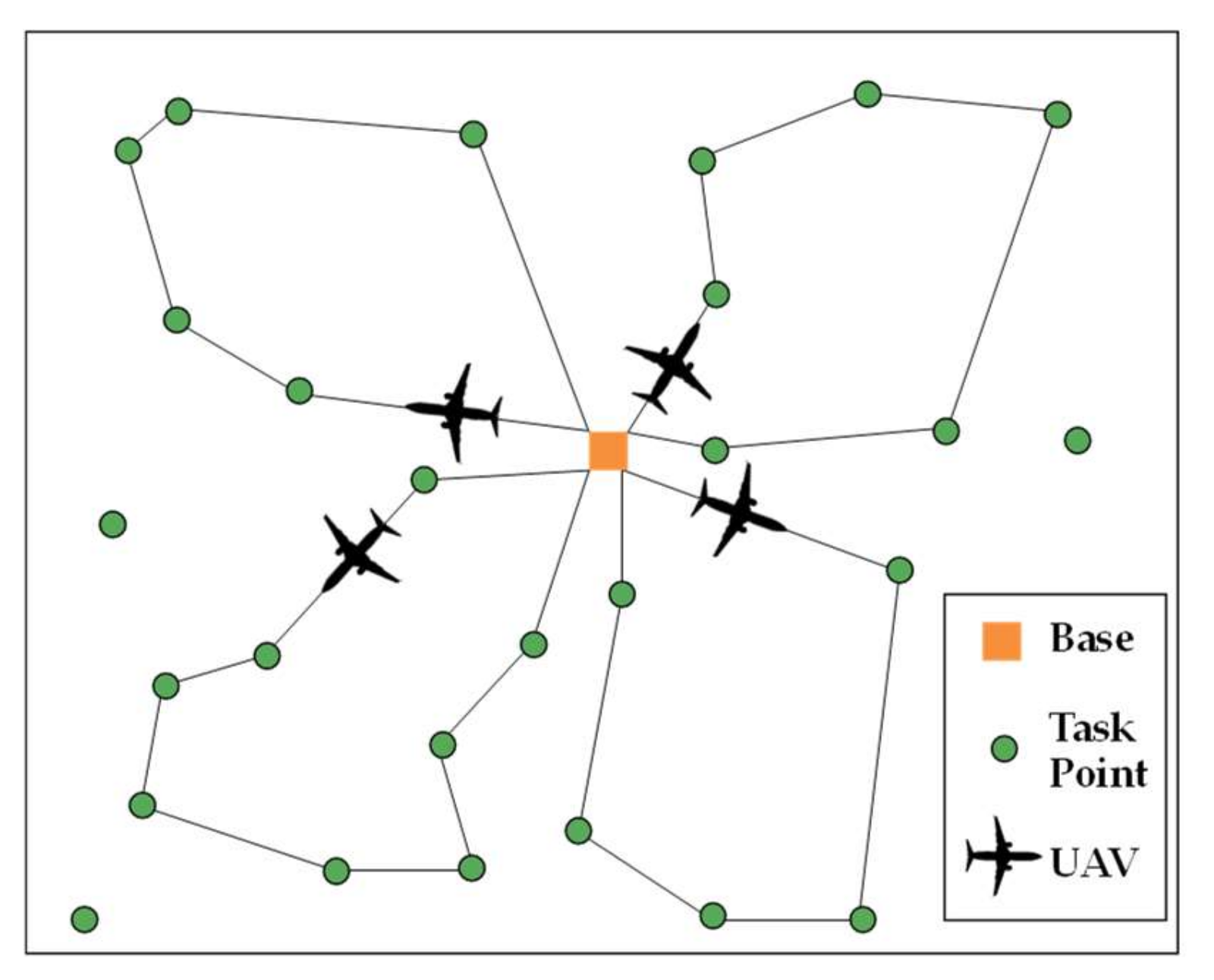
In Figure 1, there are N mission points randomly distributed in a 50 km × 50 km working area [7]. Each point is assigned a weight value based on its importance. Suppose M UAVs are deployed, and they will fly according to a planned path, collecting information such as pictures and videos taken at the mission point during the flight. Eventually, the UAVs returned to the starting point, and the data collection mission finished. During a mission: Each mission point is captured at most once during a mission. The time for mission completion is as follows: the timing starts from the first UAV taking off and ends when the last UAV returns. The main parameters in this paper are listed in Table 2.

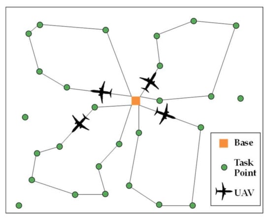
Figure 1. Environmental Model.

Table 2. Main parameters of this paper.

Definition	Symbol
The distance between mission points i and j.	${\mathit{d}}_{\mathit{ij}}$
UAV turning angle at mission point j.	${\mathsf{\theta }}_{\mathit{ijP}}$
The linear speed of UAV.	V
The angular velocity of the UAV.	ω
The flying time between mission points i and j	${\mathit{T}}_{\mathit{ij}}$
The endurance time of UAV.	${\mathit{T}}_{\mathit{max}}$
The time consumed to return to base from point j.	${\mathit{T}}_{\mathit{back}}$
Determining whether a UAV has exceeded its service life.	${\mathit{T}}_{\mathit{judge}}$
The flying time of the k-th UAV.	${\mathit{T}}_{\mathit{k}}$
Task completion time.	${\mathit{T}}_{\mathit{done}}$
The cost between mission points i and j	COSTij
The weight of mission point.	W
Weight of task coverage.	${\mathit{W}}_{\mathit{t}}$
Weight of the total area.	${\mathit{W}}_{\mathit{total}}$
Coverage rate.	$\mathit{\mu }$
The probability of an ant choosing a path.	${\mathit{P}}_{\mathit{ij}}^{\mathit{g}}$
The pheromone concentration between mission points i and j.	${\mathit{\tau }}_{\mathit{ij}}$
The reciprocal of the distance between mission points i and j.	${\mathit{\eta }}_{\mathit{ij}}$
The secondary advantage point in the COST set.	sa

3.2. Model Formulation

Definition 1

(Flight path, ${\mathit{d}}_{\mathit{ij}}$). When the UAV flies directly from mission point i to mission point j, the vector $\overrightarrow{\mathit{ij}}$ is defined to represent the flight path of the UAV, where the Euclidean distance [42] between two points is ${\mathit{d}}_{\mathit{ij}}$ as the flight distance.

$${\mathit{d}}_{\mathit{ij}}=\sqrt{{{(\mathit{x}}_{\mathit{i}}{ - \mathit{x}}_{\mathit{j}})}^2{+(\mathit{y}}_{\mathit{i}}{ - \mathit{y}}_{\mathit{j}}{)}^2}, \forall \mathit{i},\mathit{j}\in \left\{0,1,2,\cdots ,\mathit{N}\right\}$$

(1)

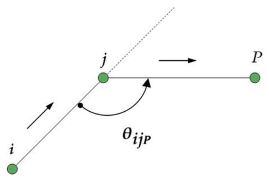
In practical scenarios, the consumption time of turning the UAV also can not be ignored. As shown in Figure 2, when the UAV moves from mission point j to the next P, the flight direction changes from $\overrightarrow{\mathit{ij}}$ to $\overrightarrow{\mathit{jP}}$ after turning by a certain angle. Therefore, the turning angle of the UAV ${\mathsf{\theta }}_{\mathit{ijP}}$ is defined as the angle between two vectors.

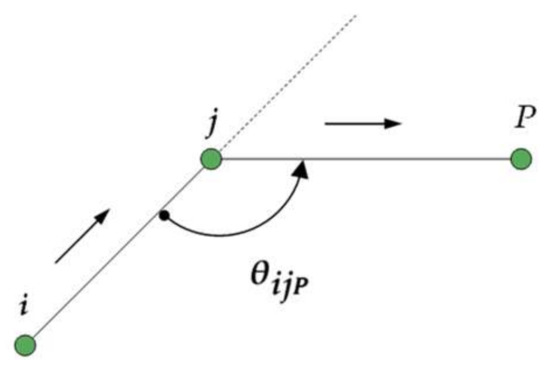
Figure 2. Turning angle diagram.

Definition 2

(Turning angle, ${\mathsf{\theta }}_{\mathit{ijP}}$).

$${\mathsf{\theta }}_{\mathit{ijP}}=\mathit{arc\; cos}\frac{{\overrightarrow{\mathit{d}}}_{\mathit{ij}}·{\overrightarrow{\mathit{d}}}_{\mathit{jP}}}{\left|{\overrightarrow{\mathit{d}}}_{\mathit{ij}}\right|·\left|{\overrightarrow{\mathit{d}}}_{\mathit{jP}}\right|},\forall \mathit{i},\mathit{j},\mathit{P}\in \left\{0,1,2,\cdots ,\mathit{N}\right\}$$

(2)

It should be pointed out that the turning angle ${\mathsf{\theta }}_{\mathit{ijP}}$ ranges from 0 to π. When the mission points i, j and P are in the same line, and the flight direction of the UAV has not changed, the turning angle ${\mathsf{\theta }}_{\mathit{ijP}}$ is 0. On the contrary, the turning angle ${\mathsf{\theta }}_{\mathit{ijP}}$ is π.

Definition 3

(Flight time, ${\mathit{T}}_{\mathit{ij}}$). Flight time refers to the time it costs for the UAV to take flight between two mission points. Assume that the UAV departs from mission point i and that the velocity is a deterministic constant. As shown in Figure 2, the flight time ${\mathit{T}}_{\mathit{ij}}$ for the UAV to travel from the current point j to the point P can be obtained by:

$${\mathit{T}}_{\mathit{jP}}=\frac{{\mathit{d}}_{\mathit{jP}}}{\mathit{V}}+\frac{{\mathsf{\theta }}_{\mathit{ijP}}}{\mathsf{\omega }},\forall \mathit{i},\mathit{j},\mathit{P}\in \left\{0,1,2,\cdots ,\mathit{N}\right\},$$

(3)

where V and ω represent the straight-line speed and turning speed of the UAV.

It is worth noting that each time a new mission point P is selected, it is necessary to predict whether there will be enough time to spend on returning to the base after reaching mission point P. Because only carrying enough energy can ensure the safety of the UAV’s flight. Therefore, it is required to calculate the estimated flight time ${\mathit{T}}_{\mathit{back}}$ from mission point P back to the base.

$${\mathit{T}}_{\mathit{back}}=\frac{{\mathit{d}}_{{\mathit{PP}}_0}}{\mathit{V}}+\frac{{\mathsf{\theta }}_{{\mathit{jPP}}_0}}{\mathsf{\omega }}, \forall \mathit{j},\mathit{P}\in \left\{0,1,2,\cdots ,\mathit{N}\right\} ,$$

(4)

where ${\mathit{P}}_0$ represents the base. It should be noted that the value ${\mathit{T}}_{\mathit{back}}$ is only to assist the algorithm in determining whether the remaining energy of the UAV is sufficient to support its return to the base.

Definition 4

(Cost function [7], COST). When the UAV selects a new mission point, it needs to calculate the energy cost function to reach this mission point.

$${\mathit{COS}\mathit{T}}_{\mathit{ij}}{=\mathsf{\epsilon }\mathit{T}}_{\mathit{ij}}+\left(1 - \mathsf{\epsilon }\right){\mathit{W}}_{\mathit{j}},\forall \mathit{i},\mathit{j}\in \left\{0,1,2,\cdots ,\mathit{N}\right\} ,$$

(5)

where ${\mathit{W}}_{\mathit{j}}$ is the weight of mission point j. ε is a constant in the range (0, 1), and it is used to balance the degree of influence of the weight and the flight time on the algorithm

Definition 5

(Total flight time, ${\mathit{T}}_{\mathit{k}}$). When the path of the k-th UAV is known, the total flight time ${\mathit{T}}_{\mathit{k}}$ of the k-th UAV can be calculated by

$${\mathit{T}}_{\mathit{k}}={\displaystyle \sum }_{\mathit{j}=0}^{\mathit{N}}{\displaystyle \sum }_{\mathit{P}=1}^{\mathit{N}}{\mathit{T}}_{\mathit{jP}}{ * \mathit{Q}}_{\mathit{jP}}^{\mathit{k}},\forall \mathit{k}\in \left\{1,2,\cdots ,\mathit{M}\right\},\forall \mathit{j},\mathit{P}\in \left\{0,1,2,\cdots ,\mathit{N}\right\} ,$$

(6)

where ${\mathit{P}}_{\mathit{jP}}^{\mathit{k}}$ indicates whether there is a path from mission point j to mission point P in the path of the k-th UAV, and if the path exists, ${\mathit{Q}}_{\mathit{jP}}^{\mathit{k}}=1$, otherwise ${\mathit{Q}}_{\mathit{jP}}^{\mathit{k}}=0$.

Definition 6

(Path weight, ${\mathit{W}}_{\mathit{k}}$). The importance of different mission points corresponds to different weights. Path weight refers to the sum of the weights of the mission points covered by the k-th UAV. The path weights ${\mathit{W}}_{\mathit{k}}$ can be obtained by calculating

$${\mathit{W}}_{\mathit{k}}={\displaystyle \sum }_{\mathit{i}=1}^{\mathit{N}}{\mathit{W}}_{\mathit{i}}{ * \mathit{X}}_{\mathit{i}}^{\mathit{k}},\forall \mathit{k}\in \left\{1,2,\cdots ,\mathit{M}\right\},\forall \mathit{i}\in \left\{0,1,2,\cdots ,\mathit{N}\right\} ,$$

(7)

where ${\mathit{W}}_{\mathit{i}}$ represents the weight of the mission point i. ${\mathit{X}}_{\mathit{i}}^{\mathit{k}}$ represents whether mission point i is covered by the k-th UAV. If the point is covered, ${\mathit{X}}_{\mathit{i}}^{\mathit{k}}=1$, otherwise ${\mathit{X}}_{\mathit{i}}^{\mathit{k}}=0$.

Definition 7

(Task completion time, ${\mathit{T}}_{\mathit{done}}$). In UAV path planning missions, task completion time and coverage rate are important metrics. The task completion time is the duration when the last UAV returns to the base. That is, the maximum value of the flight time is ${\mathit{T}}_{\mathit{done}}$.

$${\mathit{T}}_{\mathit{done}}=\mathit{max}\left({\mathit{T}}_{\mathit{k}}\right),\forall \mathit{k}\in \left\{1,2,\cdots ,\mathit{M}\right\}$$

(8)

Definition 8 (Task weight,  ${\mathit{W}}_{\mathit{t}}$).

When the paths of these k drones are known, the covered mission points can be counted. Therefore, the mission coverage weights${\mathit{W}}_{\mathit{t}}$can be obtained by calculating the sum of the weights of these mission points.

$${\mathit{W}}_{\mathit{t}}={\displaystyle \sum }_{\mathit{k}=1}^{\mathit{M}}{\mathit{W}}_{\mathit{k}},\forall \mathit{k}\in \left\{1,2,\cdots ,\mathit{M}\right\}$$

(9)

Definition 9 (Path weight, μ).

The coverage rate μ is obtained by calculating the ratio of${\mathit{W}}_{\mathit{total}}$to the task coverage weights${\mathit{W}}_{\mathit{t}}$.

$$\mathit{\mu }=\frac{{\mathit{W}}_{\mathit{t}}}{{\mathit{W}}_{\mathit{total}}} ,$$

(10)

where ${\mathit{W}}_{\mathit{total}}$ is the sum of the weights of all mission points in the mission area.

Definition 10

(Ant Colony Optimization [43] ACO). Ants secrete pheromones on their way to a mission point to obtain food, and the concentration of this pheromone can be sensed by the ants to each other. Therefore, the pheromone concentration can indicate the path distance, and the higher the density, the shorter the path length. In each iteration, the algorithm will retain the path with the highest concentration parameter. The algorithm selects the shortest path through iteration by combining group perception and a positive feedback mechanism.

$${\mathit{P}}_{\mathit{ij}}^{\mathit{g}}=\left\{\begin{array}{c}\frac{{\left[{\mathsf{\tau }}_{\mathit{ij}}\left(\mathit{t}\right)\right]}^{\mathsf{\alpha }}·{\left[{\mathsf{\eta }}_{\mathit{ij}}\left(\mathit{t}\right)\right]}^{\mathsf{\beta }}}{{{\displaystyle \sum }}_{\mathit{s}\in {\mathit{allow}}_{\mathit{k}}}{\left[{\mathsf{\tau }}_{\mathit{is}}\left(\mathit{t}\right)\right]}^{\mathsf{\alpha }}·{\left[{\mathsf{\eta }}_{\mathit{is}}\left(\mathit{t}\right)\right]}^{\mathsf{\beta }}} , \mathit{s}\in {\mathit{allow}}_{\mathit{k}}\\ 0 \hspace{1em}\hspace{1em}\hspace{1em}\hspace{1em}\hspace{1em}\hspace{1em} , \mathit{s}\notin {\mathit{allow}}_{\mathit{k}}\end{array}\right. ,$$

(11)

where ${\mathit{P}}_{\mathit{ij}}^{\mathit{g}}$ represents the probability that the g-th ant selects to travel from mission point i to mission point j; ${\mathsf{\tau }}_{\mathit{ij}}\left(\mathit{t}\right)$ represents the pheromone concentration between mission points i and j at the t-th iteration; ${\mathsf{\eta }}_{\mathit{ij}}\left(\mathit{t}\right)$ is the heuristic function whose value is the reciprocal of the distance between mission points i and j; α and β represent the pheromone concentration and the heuristic function factor, respectively; ${\mathit{allow}}_{\mathit{k}}$ represents the set of mission points which have not been visited yet. In particular, each iteration updates the pheromone concentration on the path with the following:

$$\left\{\begin{array}{c}{\mathit{\tau }}_{\mathit{i}\mathit{j}}\left(\mathit{t}+1\right)=\left(1 - \mathsf{\rho }\right){ * \mathsf{\tau }}_{\mathit{ij}}\left(\mathit{t}\right)+∆{\mathsf{\tau }}_{\mathit{ij}}\\ ∆{\mathsf{\tau }}_{\mathit{ij}}={{\displaystyle \sum }}_{\mathit{g}=1}^{\mathit{m}}∆{\mathsf{\tau }}_{\mathit{ij}}^{\mathit{g}} \end{array}\right., 0 < \mathsf{\rho } < 1 ,$$

(12)

where $∆{\mathsf{\tau }}_{\mathit{ij}}^{\mathit{g}}$ represents the pheromone concentration secreted by the g-th ant between the mission points i and j; $\Delta {\mathsf{\tau }}_{\mathit{ij}}$ represents the sum of the pheromone concentrations secreted by the total g ants between the mission points i and j. It should be pointed out that ρ is the volatilization factor and takes a range from 0 to 1. The reason is that the pheromone secreted by the ants is continuously volatilized into the air with iterations.

3.3. PCBGA Algorithm

In previous studies [7,40,41], they were calculated to get the new path point through which the UAV passed. However, when the remaining energy of the UAV does not support it to return to the base after reaching the next optimal point, the previous algorithm will decide that the UAV returns to the base directly from the current point. The above methods will lead to the energy of the UAV cannot being fully utilized.

Therefore, this paper introduces the secondary advantage point, which will be activated when the UAV encounters the content described in the previous paragraph. Then, the method will calculate the energy consumed to reach the secondary advantage point and re-evaluate whether the remaining energy is enough to support the UAV back to the base.

Definition 11 (secondary advantage point, sa).

When the mechanism of calculating secondary advantage points is activated, the energy already consumed by the UAV when it reaches the sa can be calculated by

$${\mathit{T}}_{\mathit{sa}} = {\displaystyle \sum }_{\mathit{i} = 0}^{\mathit{N}}{\mathit{T}}_{\mathit{j}}{ + \mathit{T}}_{\mathit{jsa}},\forall \mathit{j},\mathit{sa}\in \left\{1,2,\cdots ,\mathit{N}\right\} ,$$

(13)

where ${{\displaystyle \sum }}_{\mathit{j}=0}^{\mathit{N}}{\mathit{T}}_{\mathit{j}}$ denotes the time already consumed by the UAV to reach mission point j. ${\mathit{T}}_{\mathit{jsa}}$ calculates the flight time from the current mission point j to sa, where sa refers to the second mission point in the COST set. It is important to point out that when ${\mathit{T}}_{\mathit{sa}}{+\mathit{T}}_{\mathit{back}}\le {\mathit{T}}_{\mathit{max}}$, the UAV will move to sa. On the contrary, the algorithm will continue to evaluate the third smallest mission point in the COST set and so on. The UAV will return to the base if all the mission points in the COST set fail to satisfy the condition.

Algorithm Description

The details of the PCBGA algorithm are shown in Algorithm 1. First, a set of mission points P and a set of UAVs U are randomly deployed on an area, and the weight set W represent the importance mission point according to the map, as in Figure 1. Set all the UAVs to take off at the initial location of the base ${\mathit{P}}_0$ and start flying to each mission point.

Algorithm 1 PCBGA Algorithm

Input: Mission point set: ${P=\{P}_1{,P}_2,\cdots {,P}_N\}$; Weight set: ${W=\{W}_1{,W}_2,\cdots {,W}_N\}$;     $\mathrm{UAV}\mathrm{set}:{U=\{U}_1{,U}_2,\cdots {,U}_M\}$$;\mathrm{Base}:P_0$

Output: Flight path set: ${L=\{L}_1{,L}_2,\cdots {,L}_M\}$; Task completion time: $T_{\mathrm{done}}$;     Coverage rate: μ

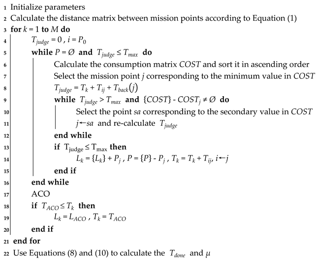In Step 1, the parameters are initialized. In Step 2, the Euclidean distance between each mission point in the task area is calculated. From step 3 to step 21, the mission points are added to the path of each UAV. In steps 6 to 7, the algorithm calculates the COST set and selects the smallest value. When the flight duration exceeds the UAV endurance time, the algorithm executes the judgment mechanism of the secondary advantage in steps 9 to 12. The set of mission points $\mathit{P}=\{{\mathit{P}}_1{,\mathit{P}}_2,\cdots {,\mathit{P}}_{\mathit{j}},\cdots {,\mathit{P}}_{\mathit{N}}\}$ is the points that need to be collected for information. In steps 13 to 15, if the mission time of point j is less than the UAV endurance time (${\mathit{T}}_{\mathit{judge}} \le { \mathit{T}}_{\mathit{max}}$), point j is added to the UAV path ${\mathit{L}}_{\mathit{k}}$. Meanwhile, point j will be removed from the mission points set P, ${\mathit{P}=\{\mathit{P}}_1{,\mathit{P}}_2,\cdots {,\mathit{P}}_{\mathit{N}}\}$. This method avoids the same point being selected repeatedly. In steps 17 to 20, the algorithm optimizes the path of the UAV using the ACO algorithm. If the new total flight time ${\mathit{T}}_{\mathit{ACO}}$ is shorter than before, the optimization of the ant colony optimization algorithm is proved successful. The path of the k-th UAV will be updated; otherwise, the original path will not be changed. After the above steps are executed, the algorithm is rerun, and the remaining mission points are assigned to the next UAV until all UAVs return to the base.

Therefore, the algorithm first uses the greedy strategy to plan the initial flight path of the UAV. When the greedy strategy determine whether the UAV needs to return to the base because of lack of energy, the suboptimal mechanism will be activated. After conducting path planning, the ant colony optimization algorithm is then used to find the optimal visiting order of the mission points that have been selected. Ultimately, the algorithm plans an efficient flight path for each UAV.

4. Simulation

The coverage performance of this algorithm is evaluated through simulation experiments. Specifically, it is evaluated by two aspects: task completion time and coverage rate. To demonstrate the superiority of the algorithm, we also use the WTSC algorithm [7] and the G-MSCR algorithm [41] as the contrast. It is important to note that the UAV collects data when it passes the mission point and does hover above it. All simulations in this chapter are performed in MATLAB, and the simulation experiments and detailed results are shown below.

4.1. Simulation Model

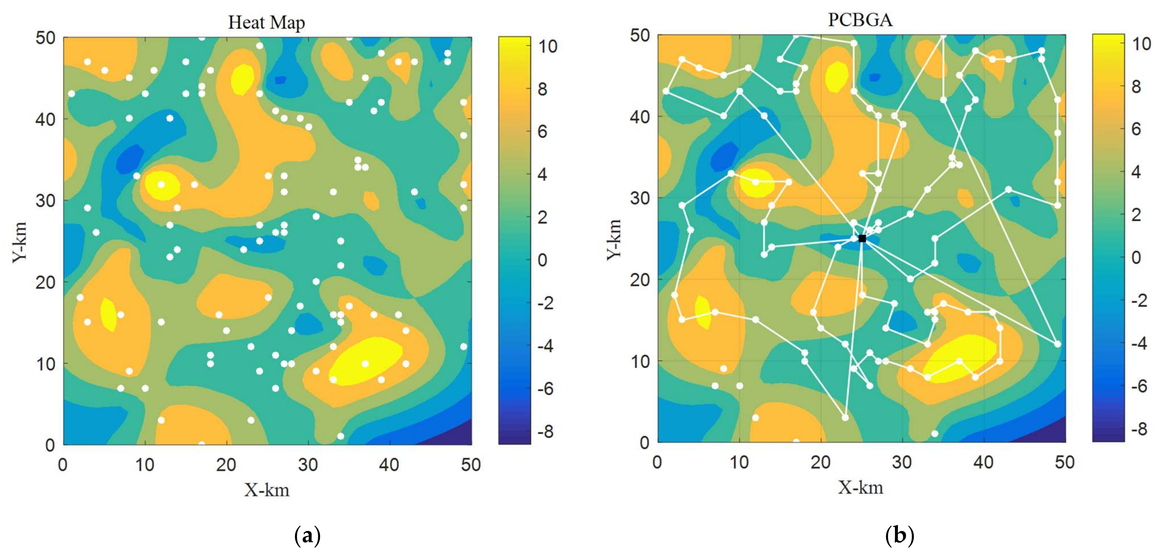
The main parameters [7] in the simulation experiment are shown in Table 3. The number of mission points is between 50 and 400. It should be pointed out that the mission points are obtained from locations in the monitored area where the heat value is higher than 0, as shown in Figure 3a. The heat value of an area indicates the probability of a disaster occurring in that area and expresses the heat value as the weight of the mission point in that area. The camera carried by the UAV has a coverage range of 1.5 km² at an altitude of 1 km.

Table 3. Simulation experiment parameter setting table.

Parameters	Value
Region	$50 \mathrm{km} \times 50 \mathrm{km}$
The number of mission point.	$50\to 400$
The weight of the mission point.	$1\to 10$
The number of UAVs.	$5\to 10$
Linear velocity	$5 \mathrm{m}/\mathrm{s}$
Angular velocity	5°/s
Flight duration	$90 \min$
Camera field of view	73.5° × 53.1°
Camera coverage	$1{.5 \mathrm{km}}^2$

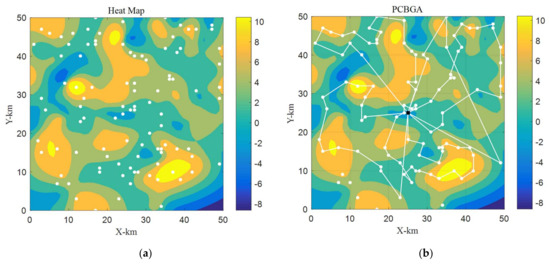
Figure 3. The path planning when N = 100, M = 5. (a) Simulation heat map of forest environment; (b) Flight paths based on the PCBGA algorithm.

4.2. PCBGA Algorithm for Path Planning on Heat Map

The experiment verifies the planning capability of the PCBGA algorithm on the heat map of the mission area. Refer to Table 2 for the environment and simulation data settings. It should be pointed out that the number M of UAVs is fixed at 5, and the number of mission points N is fixed at 100. The experimental result is shown in Figure 3b.

In Figure 3b, the black square indicates the base, the white circles indicate the mission points, and the white straight lines are the flight paths of the UAVs. The PCBGA algorithm works out the flight paths of the UAVs. The mission points in critical areas are largely covered, while less important points are not. The coverage rate is 92.13%, and the mission completion time is 87.98 min.

4.3. Performance Comparison of the Three Algorithms

Two sets of simulation experiments with different numbers of mission points and UAVs are also set up to compare the impact of the three algorithms on task completion times and coverage rates. The experimental results are counted as follows: the results of 10 executions of each of the three algorithms are counted, and their averages are calculated.

4.3.1. Comparison with Different Number of Mission Points

In this case, M is 5, and N is incremented from 50 to 400. This experiment compares the change in task completion time and coverage rate with the increasing number of mission points. The simulation results are shown in Figure 4 and Figure 5.

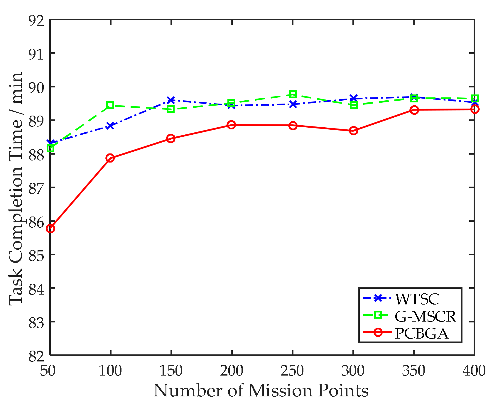
Figure 4. Comparison of the task completion time with the increase of the mission points.

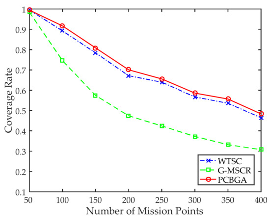
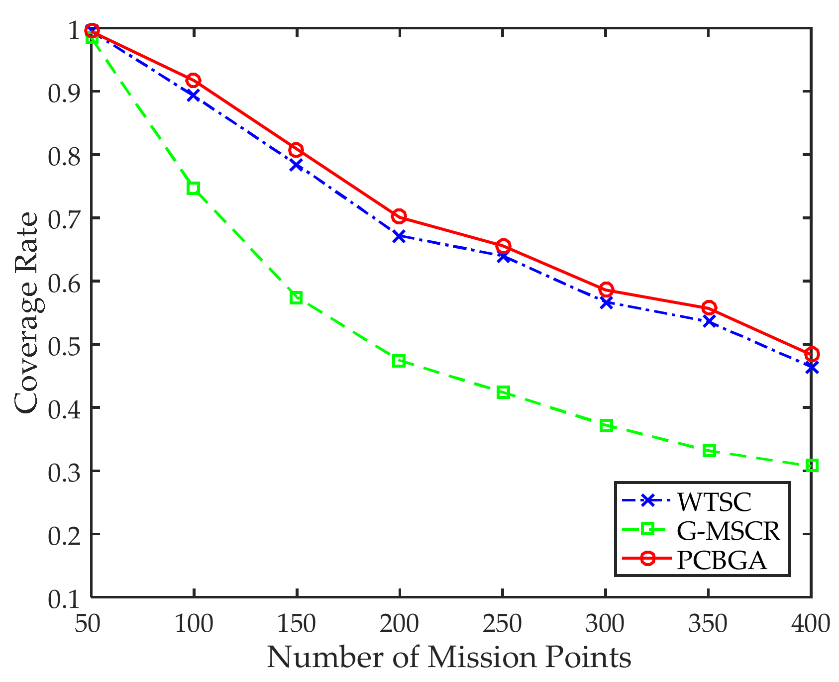
Figure 5. Comparison of the coverage rate with the increase of the mission points.

In Figure 4, the x-axis represents the number of mission points, and the y-axis represents the task completion time. It is clear from the figure that when the number of the mission points is 50, the task completion times of the PCBGA algorithm, the WTSC algorithm, and the G-MSCR algorithm are 85.77, 88.31, and 88.17 min, respectively. PCBGA algorithm takes the shortest time. The analysis shows that with the increase in the number of mission points, the task completion time of the three algorithms keeps increasing slowly. However, the task completion time of the PCBGA algorithm is always the fastest. Its task completion time is about 2.8% shorter than the other two algorithms. That is, the PCBGA algorithm performs better in the task completion time.

In Figure 5, the x-axis represents the number of mission points, and the y-axis represents the coverage rate. When the number of mission points N is 50, the task coverage rate of the PCBGA algorithm and WTSC algorithm is 99.5%, and the algorithm coverage rate of G-MSCR is 98.4%. With the increase of mission points, the task coverage of the three algorithms decreases to a certain extent. The reason is that the endurance time of a single UAV is limited. When the number of mission points exceeds a certain value, the flight time of the UAV reaches the upper limit. As the number of mission points continues to increase, more mission point coverage will not be completed. Nevertheless, regardless of the change in the number of mission points, the task coverage of the PCBGA algorithm is still the largest. It is worth noting that compared with the WTSC algorithm and the G-MSCR algorithm, our algorithm achieves a maximum improvement of 4.4% and 57.3% in task coverage, respectively.

4.3.2. Comparison with Different Number of UAVs

In this case, the number of mission points N is fixed at 200, and the number of UAVs M is increased from 3 to 10. The simulation results are shown in Figure 6 and Figure 7.

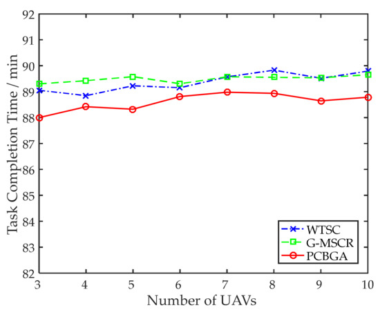
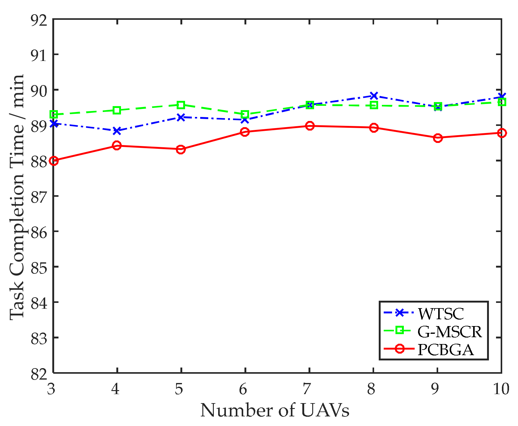
Figure 6. Comparison of the task completion time with the increase of UAVs.

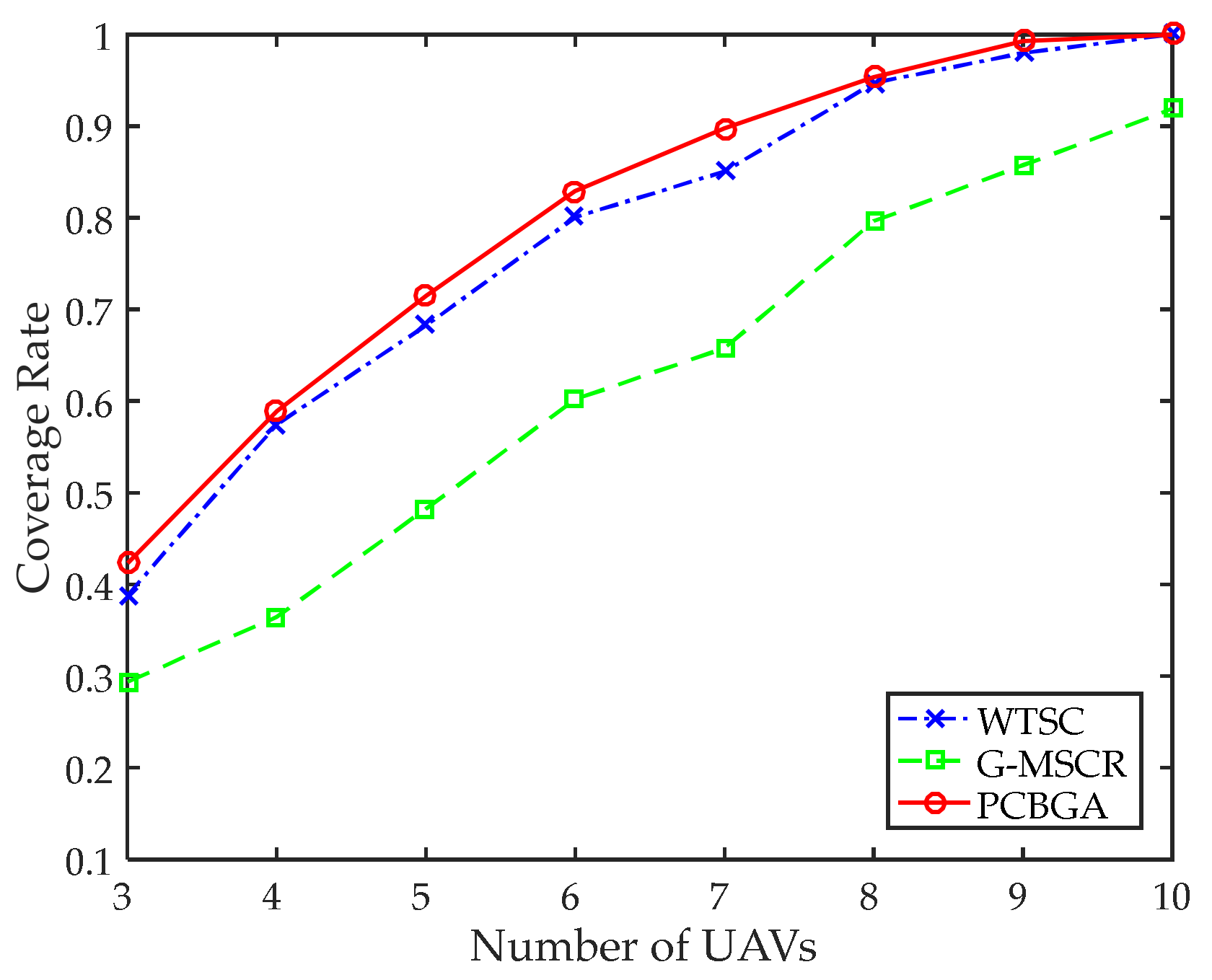
Figure 7. Comparison of the coverage rate with the increase of UAVs.

In Figure 6, the results show that when the number of mission points is 200, and the number of UAVs is 3, the task completion times for the WTSC algorithm and the G-MSCR algorithm are 89 min and 89.2 min, respectively. However, the task completion time by the PCBGA algorithm is 88 min, which is the shortest one. With the number of UAVs changing, all three algorithms remain stable regarding task completion time. This phenomenon occurs because the task completion time is defined by when the last UAV returns to the base. Meanwhile, the algorithm proposed in this paper plans the UAVs flight paths according to the takeoff sequence. In this case, the change in task completion time will remain stable when the number of UAVs increases. Nevertheless, the PCBGA algorithm is still the fastest among the three algorithms.

In Figure 7, when the number of mission points is fixed at 200 and the number of UAVs is 3, the coverage rates of PCBGA, WTSC, and G-MSCR algorithms are 0.3, 0.4, and 0.43, respectively. As the number of UAVs changes, the coverage rate of the three algorithms keeps increasing. The reason for this phenomenon is that more UAVs are involved during the work. When the number of UAVs is 10, the coverage rate of the PCBGA and WTSC algorithms is 100%. It should be pointed out that the PCBGA algorithm always maintains the highest task coverage.

Therefore, it can be seen that the PCBGA algorithm is superior to the other two algorithms. The above conclusions express that the PCBGA can effectively design the path of the UAV, improving the mission coverage while shortening the mission time.

5. Conclusions

In order to achieve efficient UAV flights planning and ensure surveillance operations in hazardous areas. The problem of concern in this paper is the inability of UAVs to balance mission completion time and coverage in large areas due to energy limitations. The proposed algorithm will seek solutions to obtain maximum coverage benefits with minimum time costs. First, the algorithm introduces a second advantage mechanism to optimize the greedy goal assignment strategy to coordinate the flight time between task points and the importance of task points to obtain the initial path. Secondly, the above initial path is continuously iterated using the positive feedback mechanism of ant colony optimization, this method optimizes the order in which these points are accessed. Finally, the proposed algorithm is compared with the WTSC and G-MSCR algorithms. The results of the experiments show that the proposed algorithm has better stability, and the objective of a higher coverage rate in a shorter time is achieved.

The real shape of the obstacles can affect the flight of the UAV to some degree. Path planning technology for UAVs needs to have online planning capability, shorter computation time, and better robustness. In the future, the authors intend to use a combination of deep learning methods and ant colony optimization to further improve the algorithm in this paper.

References

- Paden, B.; Cap, M.; Yong, S.Z.; Yershov, D.; Frazzoli, E. A Survey of Motion Planning and Control Techniques for Self-Driving Urban Vehicles. IEEE Trans. Intell. Veh. 2016, 1, 33–55. [Google Scholar] [CrossRef]
- Wu, Y.; Wu, S.; Hu, X. Cooperative Path Planning of UAVs & UGVs for a Persistent Surveillance Task in Urban Environments. IEEE Internet Things J. 2021, 8, 4906–4919. [Google Scholar] [CrossRef]
- Muñoz, J.; López, B.; Quevedo, F.; Monje, C.A.; Garrido, S.; Moreno, L.E. Multi UAV Coverage Path Planning in Urban Environments. Sensors 2021, 21, 7365. [Google Scholar] [CrossRef] [PubMed]
- Harikumar, K.; Senthilnath, J.; Sundaram, S. Multi-UAV Oxyrrhis Marina-Inspired Search and Dynamic Formation Control for Forest Firefighting. IEEE Trans. Autom. Sci. Eng. 2019, 16, 863–873. [Google Scholar] [CrossRef]
- Al-Kaff, A.; Madridano, Á.; Campos, S.; García, F.; Martín, D.; de la Escalera, A. Emergency Support Unmanned Aerial Vehicle for Forest Fire Surveillance. Electronics 2020, 9, 260. [Google Scholar] [CrossRef]
- Wang, H.; Du, H. Time Sensitive Sweep Coverage with Minimum UAVs. Theor. Comput. Sci. 2022, 928, 197–209. [Google Scholar] [CrossRef]
- Li, J.; Xiong, Y.; She, J.; Wu, M. A Path Planning Method for Sweep Coverage With Multiple UAVs. IEEE Internet Things J. 2020, 7, 8967–8978. [Google Scholar] [CrossRef]
- Aggarwal, S.; Kumar, N. Path planning techniques for unmanned aerial vehicles: A review, solutions, and challenges. Comput. Commun. 2020, 149, 270–299. [Google Scholar] [CrossRef]
- Hart, P.E.; Nilsson, N.J.; Raphael, B. A Formal Basis for the Heuristic Determination of Minimum Cost Paths. IEEE Trans. Syst. Sci. Cybern. 1968, 4, 100–107. [Google Scholar] [CrossRef]
- Julius Fusic, S.; Ramkumar, P.; Hariharan, K. Path Planning of Robot Using Modified Dijkstra Algorithm. In Proceedings of the 2018 National Power Engineering Conference (NPEC), Madurai, India, 9 March 2018. [Google Scholar]
- Zammit, C.; van Kampen, E.-J. Comparison Between A* and RRT Algorithms for 3D UAV Path Planning. Unmanned Syst. 2022, 10, 129–146. [Google Scholar] [CrossRef]
- Shivgan, R.; Dong, Z. Energy-Efficient Drone Coverage Path Planning Using Genetic Algorithm. In Proceedings of the 2020 IEEE 21st International Conference on High Performance Switching and Routing (HPSR), Newark, NJ, USA, 11 May 2020. [Google Scholar]
- Sharma, A. Swarm Intelligence: Foundation, Principles, and Engineering Applications, 1st ed.; Mathematical Engineering, Manufacturing, and Management Sciences; CRC Press: Boca Raton, FL, USA, 2022; ISBN 978-0-367-54661-8. [Google Scholar]
- Sharma, A.; Shoval, S.; Sharma, A.; Pandey, J.K. Path Planning for Multiple Targets Interception by the Swarm of UAVs based on Swarm Intelligence Algorithms: A Review. IETE Tech. Rev. 2022, 39, 675–697. [Google Scholar] [CrossRef]
- Mirjalili, S.; Mirjalili, S.M.; Lewis, A. Grey Wolf Optimizer. Adv. Eng. Softw. 2014, 69, 46–61. [Google Scholar] [CrossRef]
- Yang, X.S. Bat Algorithm for Multi-Objective Optimisation. Int. J. Bio-Inspired Comput. 2011, 3, 267. [Google Scholar] [CrossRef]
- Liu, C.; Mao, Q.; Chu, X.; Xie, S. An Improved A-Star Algorithm Considering Water Current, Traffic Separation and Berthing for Vessel Path Planning. Appl. Sci. 2019, 9, 1057. [Google Scholar] [CrossRef]
- Wang, N.; Xu, H. Dynamics-Constrained Global-Local Hybrid Path Planning of an Autonomous Surface Vehicle. IEEE Trans. Veh. Technol. 2020, 69, 6928–6942. [Google Scholar] [CrossRef]
- Gao, S.; Wu, J.; Ai, J. Multi-UAV Reconnaissance Task Allocation for Heterogeneous Targets Using Grouping Ant Colony Optimization Algorithm. Soft Comput. 2021, 25, 7155–7167. [Google Scholar] [CrossRef]
- Chen, X.; Gao, P. Path Planning and Control of Soccer Robot Based on Genetic Algorithm. J. Ambient Intell. Humaniz. Comput. 2020, 11, 6177–6186. [Google Scholar] [CrossRef]
- Pehlivanoglu, Y.V.; Pehlivanoglu, P. An Enhanced Genetic Algorithm for Path Planning of Autonomous UAV in Target Coverage Problems. Appl. Soft Comput. 2021, 112, 107796. [Google Scholar] [CrossRef]
- Qu, C.; Gai, W.; Zhang, J.; Zhong, M. A Novel Hybrid Grey Wolf Optimizer Algorithm for Unmanned Aerial Vehicle (UAV) Path Planning. Knowl.-Based Syst. 2020, 194, 105530. [Google Scholar] [CrossRef]
- Zhou, X.; Gao, F.; Fang, X.; Lan, Z. Improved Bat Algorithm for UAV Path Planning in Three-Dimensional Space. IEEE Access 2021, 9, 20100–20116. [Google Scholar] [CrossRef]
- Jayaweera, H.M.; Hanoun, S. A Dynamic Artificial Potential Field (D-APF) UAV Path Planning Technique for Following Ground Moving Targets. IEEE Access 2020, 8, 192760–192776. [Google Scholar] [CrossRef]
- Fox, D.; Burgard, W.; Thrun, S. The Dynamic Window Approach to Collision Avoidance. IEEE Robot. Autom. Mag. 1997, 4, 23–33. [Google Scholar] [CrossRef]
- Shin, H.; Chae, J. A Performance Review of Collision-Free Path Planning Algorithms. Electronics 2020, 9, 316. [Google Scholar] [CrossRef]
- Song, J.; Hao, C.; Su, J. Path Planning for Unmanned Surface Vehicle Based on Predictive Artificial Potential Field. Int. J. Adv. Robot. Syst. 2020, 17, 172988142091846. [Google Scholar] [CrossRef]
- Zhao, Y.; Zheng, Z.; Liu, Y. Survey on computational-intelligence-based UAV path planning. Knowl.-Based Syst. 2018, 158, 54–64. [Google Scholar] [CrossRef]
- Zhao, X.; Yang, R.; Zhang, Y.; Yan, M.; Yue, L. Deep Reinforcement Learning for Intelligent Dual-UAV Reconnaissance Mission Planning. Electronics 2022, 11, 2031. [Google Scholar] [CrossRef]
- Gopi, S.P.; Magarini, M. Reinforcement Learning Aided UAV Base Station Location Optimization for Rate Maximization. Electronics 2021, 10, 2953. [Google Scholar] [CrossRef]
- Chang, B.R.; Tsai, H.-F.; Lyu, J.-L. Drone-Aided Path Planning for Unmanned Ground Vehicle Rapid Traversing Obstacle Area. Electronics 2022, 11, 1228. [Google Scholar] [CrossRef]
- Cabreira, T.; Brisolara, L.; Ferreira, P.R., Jr. Survey on Coverage Path Planning with Unmanned Aerial Vehicles. Drones 2019, 3, 4. [Google Scholar] [CrossRef]
- Cho, S.W.; Park, H.J.; Lee, H.; Shim, D.H.; Kim, S.-Y. Coverage Path Planning for Multiple Unmanned Aerial Vehicles in Maritime Search and Rescue Operations. Comput. Ind. Eng. 2021, 161, 107612. [Google Scholar] [CrossRef]
- Ahmadi, S.M.; Kebriaei, H.; Moradi, H. Constrained Coverage Path Planning: Evolutionary and Classical Approaches. Robotica 2018, 36, 904–924. [Google Scholar] [CrossRef]
- Bähnemann, R.; Lawrance, N.; Chung, J.J.; Pantic, M.; Siegwart, R.; Nieto, J. Revisiting Boustrophedon Coverage Path Planning as a Generalized Traveling Salesman Problem. In Field and Service Robotics; Springer: Singapore, 2021; Volume 16, pp. 277–290. [Google Scholar]
- Cabreira, T.M.; Ferreira, P.R.; Franco, C.D.; Buttazzo, G.C. Grid-Based Coverage Path Planning With Minimum Energy Over Irregular-Shaped Areas With Uavs. In Proceedings of the 2019 International Conference on Unmanned Aircraft Systems (ICUAS), Atlanta, GA, USA, 11 June 2019. [Google Scholar]
- Biundini, I.Z.; Pinto, M.F.; Melo, A.G.; Marcato, A.L.M.; Honório, L.M.; Aguiar, M.J.R. A Framework for Coverage Path Planning Optimization Based on Point Cloud for Structural Inspection. Sensors 2021, 21, 570. [Google Scholar] [CrossRef] [PubMed]
- Kruskal, J.B. On the Shortest Spanning Subtree of a Graph and the Traveling Salesman Problem. Proc. Am. Math. Soc. 1956, 7, 48–50. [Google Scholar] [CrossRef]
- Christofides, N. Worst-Case Analysis of a New Heuristic for the Travelling Salesman Problem. Oper. Res. Forum 2022, 3, 20. [Google Scholar] [CrossRef]
- Gao, X.; Fan, J.; Wu, F.; Chen, G. Approximation Algorithms for Sweep Coverage Problem With Multiple Mobile Sensors. IEEEACM Trans. Netw. 2018, 26, 990–1003. [Google Scholar] [CrossRef]
- Liu, C.; Du, H.; Ye, Q. Sweep Coverage with Return Time Constraint. In Proceedings of the 2016 IEEE Global Communications Conference (GLOBECOM), Washington, DC, USA, 4–8 December 2016. [Google Scholar] [CrossRef]
- Jembre, Y.Z.; Nugroho, Y.W.; Khan, M.T.R.; Attique, M.; Paul, R.; Shah, S.H.A.; Kim, B. Evaluation of Reinforcement and Deep Learning Algorithms in Controlling Unmanned Aerial Vehicles. Appl. Sci. 2021, 11, 7240. [Google Scholar] [CrossRef]
- Dorigo, M.; Birattari, M.; Stutzle, T. Ant Colony Optimization. IEEE Comput. Intell. Mag. 2006, 1, 28–39. [Google Scholar] [CrossRef]
Publisher’s Note: MDPI stays neutral with regard to jurisdictional claims in published maps and institutional affiliations. |
© 2022 by the authors. Licensee MDPI, Basel, Switzerland. This article is an open access article distributed under the terms and conditions of the Creative Commons Attribution (CC BY) license (https://creativecommons.org/licenses/by/4.0/).