Camera Animation for Immersive Light Field Imaging

Abstract

Among novel capture and visualization technologies, light field has made significant progress in the current decade, bringing closer its emergence in everyday use cases. Unlike many other forms of 3D displays and devices, light field visualization does not depend on any viewing equipment. Regarding its potential use cases, light field is applicable to both cinematic and interactive contents. Such contents often rely on camera animation, which is a frequent tool for the creation and presentation of 2D contents. However, while common 3D camera animation is often rather straightforward, light field visualization has certain constraints that must be considered before implementing any variation of such techniques. In this paper, we introduce our work on camera animation for light field visualization. Different types of conventional camera animation were applied to light field contents, which produced an interactive simulation. The simulation was visualized and assessed on a real light field display, the results of which are presented and discussed in this paper. Additionally, we tested different forms of realistic physical camera motion in our study, and based on our findings, we propose multiple metrics for the quality evaluation of light field visualization in the investigated context and for the assessment of plausibility.

1. Introduction

As light field (LF) technology is rapidly advancing, its presence in the industry is continuously growing, and researchers are addressing new applications of LF capture and visualization. While the large-scale penetration of the consumer market is still a moderately long-term goal, the availability of real light field displays (LFDs) already allows experts to investigate the relevant use cases, which may progressively evolve into common daily activities of future societies. Such use cases include medical applications (e.g., radiology [1,2]), telepresence [3,4], cinematography [5], digital signage (e.g., via light field LED wall panels [6]), and many more.

The effectiveness, efficiency and general success of LF use cases fundamentally rely on visualization quality and the Quality of Experience (QoE). The latter is a complex phenomenon, which cannot be determined solely by the Key Performance Indicators (KPIs) of the visualized content and the display(s) involved in the use case. According to the Qualinet White Paper on Definitions of Quality of Experience [7], “QoE is the degree of delight or annoyance of the user of an application or service. It results from the fulfillment of his or her expectations with respect to the utility and/or enjoyment of the application or service in the light of the user’s personality and current state”.

An important factor that may contribute to the delight or annoyance of the user in LF use cases is the camera animation. Basically, it is the behavior of the camera, which specifies the perspective of the user. In a static scenario of LF visualization (i.e., the position and orientation of the camera do not vary), the perceived perspective of the scene is completely based on the viewing position of the user (i.e., the viewing angle with respect to the screen). This is not to be confused with static content, which means that the scene itself does not vary over time. An example for a static scenario with dynamic content may be a large-scale LF telepresence system [4]. While the “content” (i.e., the visualized person) is indeed dynamic, the cameras that capture the individual do not move, and thus, the perceived orientation at the other end of the system does not change either. Let us now imagine a use case in which the camera does move. This can be an LF cinema, where the presented motion picture is either captured by cameras or rendered by a computer cluster. For the sake of simplicity, let us consider the latter, as real LF cinematographic capture is a road paved with countless significant obstacles. While no scientific contribution has identified visualization-related perceptual issues of LF technology thus far, inappropriate usage of camera animation may degrade the QoE through different forms of visual discomfort. For example, in the case of stereoscopic 3D (S3D) visualization, not only camera movement may affect 3D measurement accuracy [8], but it also changes the perception of the cinematic space [9], and may greatly contribute to visual fatigue [10]. Another example for immersive 3D technologies is the case of virtual reality (VR). The work of Oh and Son [11] provides a comprehensive overview of the cybersickness that may apply to VR usage, and emphasizes how camera animation may negatively affect the user, separately discussing translation acceleration [12] and speed [13].

Apart from cinematography, other LF use cases with camera animation include training and education, digital signage, gaming, and many more. Medical use cases can be relevant as well, if instead of applying changes to the content (e.g., rotating the representation of an organ), the camera is animated. This is also applicable to specific instances of industrial use cases (e.g., prototype review) and cultural heritage exhibition.

Although a great number of the potential utilizations of LF technology requires camera animation, it has not been thoroughly investigated for LF technology yet. This is particularly relevant due to its aforementioned connection to QoE. Furthermore, as stated earlier, camera animation may also affect effectiveness and efficiency (e.g., task performance).

The aim of this scientific contribution is to apply and study camera animation in the context of LF visualization. Our work fundamentally builds on the extensive literature on camera animation that is already available for conventional 2D displays. The efforts presented in this paper take into account the limitations and challenges that apply to LF capture and visualization [14], which resulted an interactive simulation on a real LFD.

Furthermore, the implemented camera animations were extended to include realistic physical motions. Similarly to the different camera animation techniques, the realistic camera motions were simulated and tested on a real LFD. The plausibility and effectiveness of these motions were evaluated via different metrics, such as the number of collisions, occlusions, and blurry regions.

The remainder of the paper is structured as follows. Section 2 provides a quick overview of the science behind the practical applications of LF and presents the state-of-the-art LF camera technologies. Camera animation is detailed in Section 3, separately for general and for LF camera animation, including our criteria of evaluation. The visualization and assessment of LF camera animation is introduced in Section 4. Section 5 concludes the paper and highlights the potential continuations of the investigated research topic.

2. Light Field Capture and Visualization

2.1. Brief Historical Overview of Light Field

The technical term LF is known as the radiance at a point in a certain direction [15]. LFs are represented as 7D plenoptic functions that incorporate the spatial and angular information of light rays [16,17]. This function can be reduced to 5D, and in free space—in which no occluders are present—4D is considered sufficient. This is due to the fact that the radiance along a line remains unchanged unless intercepted [15]. Although this information about light distribution is indeed important, conventional cameras do not capture most of this information. However, LF cameras have the capability to re-capture the aforementioned lost information [18].

Regarding visualization, LFDs convey realistic visual experiences to spectators via the natural, glasses-free 3D perception of the content. They can be designed by means of parallax barrier and integral imaging [19]. Real LFDs have already been implemented in practice, among which are the HoloVizio displays. These displays utilize a holographic screen and a set of optical modules from which light beams are emitted. The 3D view itself is composed by the holographic screen at which these beams arrive [20].

Before valiantly jumping in medias res of the technical details, let us review the greatest milestones that let us arrive at this point. Throughout history, numerous attempts have been made to formulate visual elements in relation to the visual information of the world. In order to extract such information, lights rays filling a part of space are inspected. The most notable attempts for this were the following:

• Leonardo da Vinci described light rays filling space as “radiant pyramids” that intersect and cross one another [21].
• Michael Faraday used the term “lines of force” to describe light rays, claiming that LFs are more or less analogous to magnetic fields [22].
• Frederic E. Ives managed to record parallax stereograms in 1903 by means of a single-lens apparatus [23].
• LF photography was first introduced by Gabriel Lippmann in 1908. He provided the theoretical foundations for LF photography under the name of “integral photography” [24], and proposed a setup where multiple crystalline lenses are placed hexagonally—similarly to a beehive.
• In 1939, Arun Gershun introduced the term “light field” to describe light rays filling space by their radiometric properties [25].
• The first plenoptic camera was proposed by Edward Adelson and John Wang in 1992, consisting of a single lens and a sensor plane, in front of which a lenticular array was planted [26].

The most recent works on LF visualization include novel display systems such as the Aktina Vision [27], the aforementioned LF LED wall [6], one solution with a space-multiplexed voxel screen [28] and one with a ladder-compound lenticular lens unit (LC-LLU) [29]; various camera systems [30,31,32]; compression methods [33,34,35]; view synthesis [36,37,38]; reconstruction [39,40,41]; objective quality assessment [42,43,44]; subjective studies [45,46,47]; and the advances of JPEG pleno [48]. Regarding LF QoE, while the vast majority of the scientific literature focuses on perceptual thresholds and personal preference [49,50,51,52,53,54], the research questions of future works will address immersion, interaction, human-computer interface (HCI), inter-user effects, perceptual fatigue, super resolution, and many more [55].

2.2. Classification of Light Field Displays

Today, the devices of projection-based LF visualization are grouped into the categories of horizontal-only parallax (HOP) and full-parallax (FP; do not confuse with First-Person cameras, also abbreviated by FP) displays. On a theoretical level, vertical-only parallax (VOP) displays are feasible as well, and they are precisely as complex as HOP displays, but the horizontal separation of the human eyes and the primarily horizontal movement in potential use cases make HOP displays significantly more relevant.

FP displays can visualize contents recorded by FP cameras, while HOP displays evidently need to select a subset of the content. In practice, high-quality visualization demands that the capture device and the display device have LFs that match as much as possible.

The baseline for a camera system arranged as a linear array is the Euclidian distance between the leftmost and the rightmost camera. As this metric is crucial for the operation and assessment of LF cameras in general, our work extends to other types of LF camera systems as well.

2.3. Camera Setups for Light Field Displays

Let us now define the capture surface of an LF camera. First, we determine a set of points by taking the individual spatial positions for each sensor per pixel. Then, we can tessellate a piece-wise flat spanning surface between the neighboring points to obtain the capture surface.

The normal of the capture plane is the average of the camera direction vectors. This scientific discussion excludes camera systems with any two rays that have an angle larger than ±90 degrees, as such systems should always be treated as 2 or more separate systems from this perspective. The plane contains the point of the capture surface for which the dot product of the point with the normal vector of the capture plane is minimal.

We define the capture rectangle by evaluating the intersection points of all light rays measured by the LF camera with the capture plane, and by calculating the axis-aligned bounding rectangle around them. We call this bounding rectangle the as capture rectangle. Please note that in the 1D linear case, the capture rectangle and the baseline are one and the same.

HOP LF cameras can be differentiated further into narrow-baseline (baseline shorter than 1 m) and wide-baseline LF cameras. Due to having smaller baselines, narrow-baseline LF cameras are more portable compared to wide-baseline LF cameras [14]. On the other hand, reconstruction accuracy is limited in narrow-baseline LF cameras since accuracy is linearly proportional to the baseline. Moreover, narrower baselines lead to “sub-pixel feature disparities”, resulting in the deterioration of spatial resolution [56,57]. Since both the angular and spatial information are captured by LF cameras for light rays, LF images provide easier methods for depth map estimation [17]. Analogous to the aspect of accuracy, wide-baseline LF cameras are better in depth map estimation since the baseline is inversely proportional to the depth estimation error [56].

LFDs provide a naturally-wide baseline due to their large screen size $S_{x,y}$, optimal observer distance $D_{observer}$ (usually 1 to 4 m, depending on screen size and the choice of vertical perspective [58]), and outward facing light emission angle $FO{V}_{xdisplay}$ (45 degrees to 170 degrees). For HOP systems with a planar screen—as seen in Figure 1—baseline $B_{xdisplay}$ corresponding to an LFD can be calculated as:

$$B_{xdisplay}=2\ast D_{observer}\ast tan(\frac{FO{V}_{xdisplay}}{2})+S_x$$

(1)

In general, the more a camera system covers the whole baseline during the measurement of the LF, the better match it is going to be for the LF of the display—assuming the same camera count and camera parameters, such as resolution and field of view (FOV). As baselines are typically in the range of 3 to 24 m for practical display sizes, LFDs are optimally matched by wide-baseline cameras.

Table 1. Comparison between narrow-baseline and wide-baseline light field cameras.

	Narrow-Baseline Light Field Cameras	Wide-Baseline Light Field Cameras
Length	Measured in centimeters (less than 1 m)	More than 1 m
Reconstruction accuracy	Limited and can lead to sub-pixel feature disparities	Better
Depth map estimation	Limited	Better
Spatial resolution	Deteriorated	Enhanced
Portability	Relatively portable	Not portable

sums up the differences between narrow-baseline and wide-baseline LF cameras.

In practice, LF cameras are either plenoptic cameras or arrays of pinhole cameras. In the case of conventional cameras, an object space point is projected into a single pixel. For plenoptic cameras, a light ray emitted from a point is projected to many positions of the sensor [59]. The plenoptic camera is trivially named after the plenoptic function itself. In their studies to discover how the human visual system (HVS) is capable of extracting the geometric information from the viewed images, Adelson and Bergen introduced the plenoptic function which defines the “total geometric distribution of light” [60]. Plenoptic cameras were made commercially available by Lytro (until 2018), and are still available for purchase from Raytrix (https://raytrix.de/ accessed on 1 August 2022).

As the name implies, camera arrays are multiple cameras that are arranged in arrays to capture the same scene in a synchronized manner. Several possible arrangements can be done, for instance, HOP camera arrays—usually arranged in a linear or arc setup—or FP camera arrays—usually arranged on a 2D grid or spherical arrangement. Camera arrays can be built in various configurations from any type of industrial camera that has a synchronization port. For example, LF camera arrays are offered by Fraunhofer IIS (https://www.iis.fraunhofer.de/en/ff/amm/for/forschbewegtbildtechn/lichtfeld.html accessed on 1 August 2022).

To determine how well a camera system performs on an LFD, we need to establish an error metric. First, we have to define the observer rectangle (observer line for HOP) for the LFD. This rectangle lies on the observer plane, which is parallel to the display plane. The observer rectangle is the minimum axis-aligned bounding rectangle of all intersection points of emitted rays and the observer plane.

Then, we convert all camera rays into a Cartesian coordinate system, where we have defined the mathematical representation of the display rays and the observer rectangle, using a 4 × 4 affine transformation matrix, also known as the region of interest (ROI) matrix [61]. The coordinate system places the display plane on an $xy$ plane at $z=0$. We further restrict the parameters of the ROI matrix to contain uniform scaling, and we want to set the matrix in such a manner that after the transformation, the observer plane and the capture plane are equivalent. We recalculate the capture rectangle in the new coordinate system. It is easy to see that the only valid display rays—for which we can reliably render from the captured camera rays—lie in the intersection of the observer rectangle and the capture rectangle.

The closest camera ray to a display ray can be found by finding the minimum of the following sum for each camera ray: sum of the distance of the camera ray intersection with the display surface to the display ray’s emission point and the distance of the display ray’s intersection point with the observer plane and the camera ray’s eye position.

An error metric for a set of camera rays, an ROI, and an LFD with a planar surface can be determined as:

$$E_{{dray}_n}=\frac{1}{4}(\frac{abs(O_{{d_n}_x}-I_{{c_n}_x})}{S_x}+\frac{abs(O_{{d_n}_y}-I_{{c_n}_y})}{S_y}+\frac{abs(I_{{d_n}_x}-O_{{c_n}_x})}{S_{in{t}_x}}+\frac{abs(I_{{d_n}_y}-O_{{c_n}_y})}{S_{in{t}_y}})$$

(2)

for all $n\in N_i$ and

$$E_{capture}=\frac{{\sum }_{n\in N_o}^{}1+{\sum }_{n\in N_i}^{}{E}_{{dray}_n}}{N},$$

(3)

where N is the total number of display rays; $N_i$ is the set of display rays inside and $N_o$ is the set of display rays outside the intersection of the observer rectangle and the capture rectangle; $S_{int}$ is the (2D) size of the intersection rectangle; S is the (2D) size of the display surface; $O_{d_n}$ is the origin of the nth display ray; $I_{d_n}$ is the intersection point of the display ray and the observer rectangle; $O_{c_n}$ is the closest camera ray origin to the nth display ray, $I_{c_n}$ is the closest intersection point to $O_{d_n}$ on the display plane of all camera rays with origin $O_{c_n}$; x and y denote the x and y components of the points and sizes. Figure 2 illustrates the camera space and display space.

To extend this metric to LFDs with non-planar surfaces, Euclidian points and distances measured on the display plane and divided by the display size need to be replaced with $u,v$ surface-normalized parametric points and distances. Distances inside the projected area of the pixel on the observer plane and the emission surface on the display surface, respectively, can be treated as zero to improve the metric. In the case of additional color mixing from multiple camera rays, the metric can be extended to include all selected camera rays for a display ray and $E_{{dray}_n}$ needs to be weighted by the weights used for mixing color from the chosen camera rays.

From this metric, it is easy to see that it would be extremely difficult to build LF capture systems for most LFDs where $E_{captureROI}=0$ holds true. However, it is straightforward to define new virtual cameras (sets of capture rays that match the display rays exactly) for any given ROI transform of a virtual scene that matches the criteria for the ROI transforms listed above. Therefore, using virtual cameras is a superior option to test camera-related problems, as they are both easy to place and move using only the ROI matrix and they are free from capture error by definition.

3. Camera Animation

3.1. General Camera Animation

3.1.1. Cinematography Camera Animations

Among the main components of cinematography are camera movements and shots, which play important roles in storytelling. In this section, we discuss the most relevant types of cinematographic camera movements.

Pan is short for panoramic. It describes the left and right horizontal camera movements without changing the position of the camera. However, the strobing effect arises when the camera is being moved too fast, which accounts as a limitation for the pan movement itself.

Similarly to pan, tilt does not change the position of the camera. Yet, unlike pan, tilt describes the vertical (up and down) motion of the camera. Furthermore, it needs to be stated that tilt is not used as frequently as pan since the majority of events in everyday life (and thus in cinematic content) occur along the horizontal plane.

The camera movement known as zoom encompasses an optical change in focal length. In the world of cinematography, it is crucial that zoom is only used when such visual method is necessary (i.e., carries meaning for artistic and/or storytelling purposes). Moreover, hiding or suppressing zoom is somewhat advisable in order to avoid drawing the attention of the audience to the zoom effect, as it may degrade immersion. This can be achieved by combining zoom with other camera movements, such as pan, dolly or tilt, or with certain movements of the actors and objects in the scene.

Dolly is often called “move in/move out” and “push in/push out”. The move in/out camera movement combines both the wide and the tighter shots of the scene. This movement is used to focus the attention of the audience efficiently rather than cutting the scene from a wider to a closer shot. There are also many other cinematic uses for this type of camera movement. For example, dolly is commonly used as a form of pulling back from a scene upon the entrance of an actor. During this type of dolly, the camera moves towards or away from the subject of interest. Unlike zooming, the camera is a wheeled cart (or mounted on a track/motorized vehicle), so the camera itself moves. This gives a sense of world movement around the subject. In other words, the background appears to be moving behind the subject, which further enhances the sense of motion.

Truck movement is rather similar to dolly. However, it moves the camera horizontally (left and right) instead of in and out. This type of camera motion is typical for the cinematic use of following a moving entity (e.g., a character in action).

In the case of pedestal—similarly to the concept of dolly and truck—the camera moves, but this movement is vertical (up and down). It is frequently used to capture tall/high entities (e.g., the cinematic introduction of a tall character or a tall building).

3.1.2. Simulation Camera Animations

These types of camera animation are used extensively in video games, where the player interacts with and perceives the surrounding environment by means of virtual cameras. For perceiving the virtual world from a certain perspective, the main components of a camera system have to be set (i.e., the position and the orientation of the camera) [62]. In this part of the section, we discuss the most relevant types of simulation cameras.

Fly/Walk/Point-of-View (POV)/First-Person (FP) cameras are most commonly used in video games. The idea is to view the scene from the perspective of the character, the avatar of the player, or the player-controlled vehicle (e.g., first-person cockpit view or view from the front of the vehicle). This technique appears in a multitude of video game genres, among which first-person shooters (FPS) and driving/flying simulators are very well known. Hence, the technique of FP camera can provide a significant sense of immersion. Although FP cameras may add reality to the game, its field of vision is rather limited. Furthermore, in addition to video games, FP cameras are sometimes used in cinematic content to present the perspective of a given character. Such storytelling techniques are also referred to as the POV shot [63].

The idea of Second-Person (SP) camera animation is to view the entity of interest from the perspective of another entity. For example, the main character is viewed from the perspective of a different character. This camera was incorporated in games such as Battletoads (©Masaya, 1991), where the fight is viewed from the POV of the opponent.

Unlike FP and SP cameras, Third-Person (TP) cameras are separated from the focus of the entity of interest. In this case, the context of the game is viewed from the perspective of an external position (i.e., a virtual camera) and not from the perspective of an actual entity.

Orbiter cameras always have their “lookat” point at the center of the bounding volume of the object of interest. The camera can rotate around this fixed point on a sphere with a fixed radius. In some implementations, it is possible to change the length of the radius or to scale the scene to achieve close-up or zoom-like effects. Such cameras are often used in industrial and medical applications.

3.2. Camera Animation Design for 3D Displays

Camera interaction for 3D displays varies on a case-by-case basis, but for most solutions, it sticks to a single-interaction type. Head-mounted augmented reality (AR) and VR devices almost exclusively use the FP camera model. Volumetric displays usually opt for orbiter camera interactions. The only exception to this rule is the case of S3D cinema, which retains its richness of expression and uses all camera movements that do not change the focal length. Changing the focal length would require a change in the baseline (or lenses) and a possible calibration of the system. Recalculating the stereo base is usually calculated with the Bercovitz formula [64] as:

$$B=P\frac{L\times N}{L-N}(\frac{1}{F}-\frac{L+N}{2L\times N}),$$

(4)

where B is the stereo baseline; P is the parallax aimed for; L is the far clipping plane; N is the near clipping plane; F is the focal length of the lens. The only exception to this rule is the case of animated movies, where calibration is not required and the frame-by-frame changes in baseline or lens parameters are not an issue. Moreover, the cameras with asymmetric perspective that converge on a virtual screen can be used to provide a higher-quality stereoscopic image pair. The same stereo camera rigs are equipped with apparatus to change the baseline and consequently the focal length; however, most directors would prefer to cut due to the fact that this operation changes the “flatness” of on-screen objects.

3.3. Light Field Camera Animation

As stated earlier, LF cameras are used to capture information about light distribution. In other words, for each ray arriving at the sensor, its amount of light is captured [18]. In our case, the LF of a virtual scene is captured by an error-free virtual LF camera. Camera movement is facilitated through the ROI matrix. In practice, display rays are evaluated once and are transformed with the inverse of the ROI matrix to be in world space. As all other virtual objects and lights are also in the same coordinate system, we can easily render the individual rays.

Previous works on LF virtual camera animation for LFDs involved orbiter cameras or cameras using scene-centered rotations with dolly and truck without camera-scene interactions [65,66]. By implementing the various camera animation types, we can evaluate their usefulness for LF visualization. We generated animations for some typical scenarios used in cinematography, where we included an object of interest for the film, which is especially important for the FP and TP cases.

The following criteria were used to evaluate usefulness:

• General visibility of the scene along the observer line during animations.
• Frequency of immersion-breaking occluders.
• Frequency of collisions and course corrections within the scene.
• Frequency of depth-related artefacts.
• Occurrence of depth of field changes.

The implementation is flexible enough to work across a whole range of LFDs, specifically lenticular and projection-based ones. It was built by using the clustered rendering modules of Holografika. It also used the Bullet Physics library [67] to provide a level of realism for the scene. The application is implemented as a testing framework, where any combination of existing scenarios’—namely camera motion—scene and scene-dependent interactions can be rendered in real time to aid the evaluation. Our findings can be directly applied to the motion and operation of physical LF cameras with comparable baselines, observing the scaling factor of the ROI transform, when capturing for scenes with comparable aspect ratios.

4. Visualization of Light Field Camera Animation Used in Cinematography

In our work, camera animations by means of virtual cameras were implemented and tested on a real LFD, namely the HoloVizio C80 (https://holografika.com/c80-glasses-free-3d-cinema/ accessed 1 August 2022). This LFD has an aspect ratio of 16:9 with a screen size of 3 m × 1.8 m, hence being the perfect candidate for testing camera animations due to its sheer size, simulating a cinema screen. The viewing angle of the screen is 45 degrees with a brightness of 1000 cd/m². The tested scenes consisted of simple 3D shapes, including a generic ground, boxes, cylinders, planes, cars, and suspension elements. In order to simulate the physical properties of the modelled shapes, the “Bullet Physics Library” was used.

4.1. Simulation Camera Animations

First, we simulated and tested the different camera animation techniques mentioned in Section 3.1. By using the aforementioned elements for scene composition, we created an aisle of columns, between which a car was moving forward. The animated content was generated via a C++ code that was directly run by the renderer of the LFD (i.e., no additional software was used to model and render the source views of the scene, and thus, there was no need for conversion). The investigated camera animations were pan, tilt, zoom, dolly, truck, and pedestal. Figure 3 depicts the visualization of camera animations on the LFD (captured by a regular pinhole camera during operation). In order to get a better overview of the scene from multiple perspectives, orthographic views were added. Figure 4 shows the orthographic camera views for the scene. In addition to testing cinematographic camera animations, simulation camera animations were tested as well. Figure 5 shows the simulation camera animations (FP and TP cameras).

Discussion and Assessment

As a result of visualizing the different camera animations on the LFD, a series of inferences could be made. As discussed earlier, a set of criteria was used to evaluate camera animations. Those include general visibility, frequency of immersion, collision and depth-related artefacts, and the occurrence of depth of field changes.

The perceptual assessment was carried out via expert evaluation. In this context, this means that various light field experts of the institution rated the investigated aspects of the different camera animations, choosing from a set of descriptive, subjective options for each aspect (e.g., collision frequency was either none, low, medium or high). The evaluations were based on the plausibility of the visualized content on the LFDs, as well as prior expert knowledge of the optical limitations and challenges of LFDs. A total of 5 experts (4 males, 1 female; age range between 29 and 66; average age 42) completed the evaluation, the results of which are presented in

Table 2. Results of camera animations visualized on the light field display.

Camera Animation	General Visibility	Occluder Frequency	Collision Frequency	Depth-Related Artefacts’ Frequency	Expected Depth of Field Changes Not Occuring
Pan	Good	Low	None	Low	N/A
Tilt	Mediocre	None	Medium	High	N/A
Zoom in	Mediocre	None	High	High	Yes
Zoom out	Mediocre	Low	Low	Low	Yes
Dolly in	Mediocre	None	High	High	N/A
Dolly out	Mediocre	None	Low	Low	N/A
Truck	Good	Low	None	Low	N/A
Pedestal	Mediocre	High	Medium	Medium	N/A
FP	Bad	None	High	High	N/A
TP	Mediocre	None	High	High	N/A

. For a subjective study with naïve test participants—where quality ratings are collected via a standardized assessment scale and then statistically analyzed—the results of 5 individuals would not be considered sufficient, particularly due to the potential rating deviation. In the scope of this work, expert test participants classified visualization attributes based on a specified set of descriptors (e.g., None, Low, Medium and High for frequency), and after the tests, they had to reach a consensus for each of the 50 items.

Starting off with the cinematographic camera animations, the pan and truck movements turned out to have the best general visibility, followed by tilt, zoom, dolly, and pedestal. Occluder frequency is the rate by which the camera is occluded throughout its animation. Pan, zoom out, dolly out, and truck camera animations had the lowest occluder frequency, followed by tilt and pedestal. However, the highest occluder frequency was noticed in the case of zoom in and dolly in motions. Collision frequency is the rate by which the camera collides with objects from the scene when being animated and would need to stop, land or change trajectory. Collision is not expected for this scene, only for the pedestal case, as the one and only collider in the scene is the ground. Camera collision can be implemented for LF visualization in several different ways. It can be evaluated in world space against the bounding volume of the LF, the axis-aligned bounding box of the bounding volume, the ROI box, the center of the ROI box, the observer line or the axis-aligned bounding rectangle of the intersection points of display rays and the maximum addressable depth plane towards the observers. The current implementation used the observer line for collision, as this behavior matches that of a physical LF camera system the best. Depth-related artefacts arose when objects that were previously in the right range of depth for sharp visualization got close or over the range for the sharp region of the depth of field. Due to the arrangement of objects in this scene, this metric follows the occluder frequency quite closely. For some cases, such as tilt, the amount of ground that is visible changed significantly, resulting in more artefacts, while keeping the number of occluders similar throughout the motion sequence. For dolly out, this occurrence of depth-related artefacts became smaller in the back, and more frequent in the front. For dolly in, the opposite applied. As for 2D camera animations, zooming in and out results in the change of the camera’s focal lens. Although the same effects are expected to occur when utilizing zoom on LFDs, change in the focal lens is, of course, not possible when using LF. Accordingly, the expected changes in the depth of field when zooming did not occur. In order to produce something similar to the zoom effect, the extents of the ROI were scaled.

Moving on to the simulation camera animations, the FP and TP cameras were implemented and tested. The general visibility for the FP camera was poor; however, it was better for the TP camera. Both FP and TP cameras resulted in high rates for occluders, collision and depth-related artefacts. As illustrated in the figures, some camera animations led to plausible results on the LFD, while others were lacking. Among the cinematographic camera animations, pan, tilt, truck, and pedestal camera movements resulted in satisfactory outputs. However, blurriness artefacts were present for dolly and zoom towards the scene. The same applied to FP camera when testing simulation camera animations. On the other hand, TP cameras resulted in plausible results as well.

4.2. Realistic Physical Camera Animations

For the vast majority of action movies, dynamic shots are of utmost importance. Of course, this statement is applicable to movies of other genres as well. Depending on the complexity of the shot, one or more cameras are deployed to record the scene. These cameras may be so-called steadycams, certain cameras may be mounted on objects in motion, and the capture procedure might require several camera operators. As an extension to our work, in order to further study the perceptual impact of such complex dynamic shots on LFDs, various realistic physical camera animations were simulated and tested on the HoloVizio C80 LFD. The primary motivation was to simulate some of the realistic motions that are common in cinematography by means of virtual LF cameras.

In order to test the physics simulation on the LFD, three test cases (i.e., scenarios) were implemented (see Figure 6):

• Collision camera: The first scenario consists of a car and a set of columns, into which the car is moving. The car accelerates on its way towards the columns, resulting in its collision with one of them. The camera is mounted twice on the car as an FP and as a TP camera, and once on the collided column.
• Suspension camera: In this scenario, the camera is mounted once on a suspension object with the car placed in front of the suspension element and once on the car itself, looking towards the suspension element.
• Falling camera: In this scenario, a camera is falling from an altitude towards the ground until it collides with the latter. There is a total of 50 objects (boxes and cylinders) on the ground.

4.2.1. Metrics

In order to test the plausibility and efficiency of the resulting physical camera simulations on the LFD, various metrics were used [68]. The following sums up these objective metrics:

• Collisions: Since we used physical camera motions in our study, there was the possibility of the collision of the camera with the objects from the scene. Counting the number of collisions between the camera and the objects was carried out to decide whether or not this camera motion would provide plausible results.
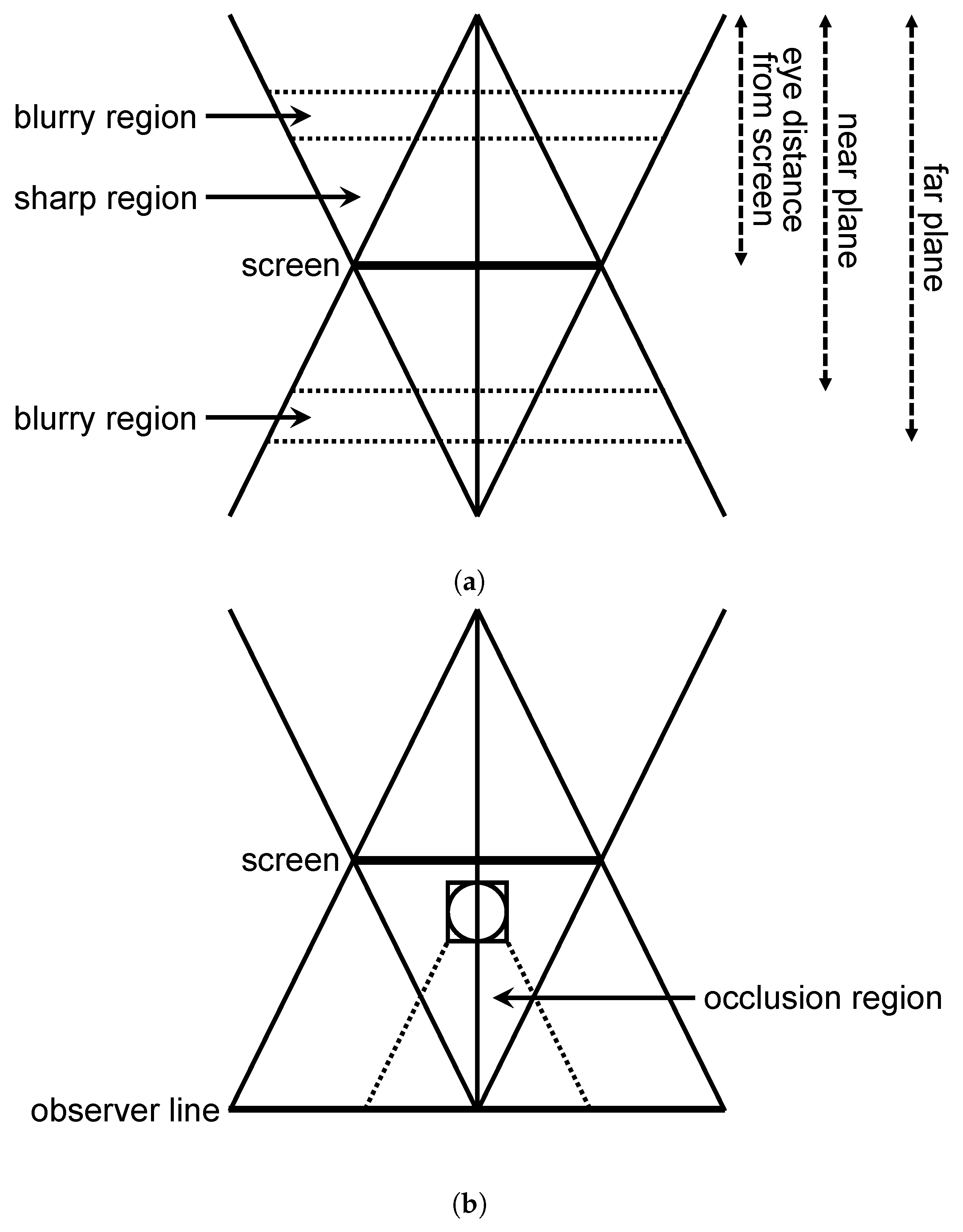
• Blurry region: Figure 7a shows the top view taken from the LFD setup. Unlike conventional displays, LFDs have double frustums placed in front of and behind the screen, illustrated with the black line. The viewing angles enclosing the frustums are depicted by the blue lines. Considering LFDs, the area enclosing the screen contains the objects that are sharply rendered. In this metric, we calculated the number of objects that were rendered outside the sharp region.
• Occlusion region: When using TP cameras, this metric is used to count the number of objects occluding the main entity with respect to the camera. Figure 7b shows the top view of the setup illustrating this metric, where the main entity is shown as the yellow circle. The main entity is enclosed by an axis-aligned bounding box (AABB), illustrated with the red square. In order to measure the number of objects in the occlusion region, the latter should be set up prior to the assessment. The occlusion region is depicted by the frustum drawn in front of the main entity, illustrated with blue lines. The back plane of the frustum is the same plane as that of the front of the AABB of the main entity. The right and left planes enclosing the frustum are parallel to the viewing angle planes of the LFD. However, they enclose the main entity. Finally, the top and bottom planes are constructed starting from the top and bottom lines of the AABB of the main entity and passing by the observer line. Once the occlusion region is constructed, the number of objects within are calculated by counting the number of intersections between the frustum depicting the occlusion region and the AABBs of the elements in the scene.

4.2.2. Evaluation and Testing

In order to check the plausibility of the produced physical animations on the LFDs, the realistic physical scenarios discussed in Section 4.2 were tested against the metrics discussed in Section 4.2.1. The results of the tests are summarized in

Table 3. Metrics tested for realistic physical camera simulations.

Scenario	Number of Objects Colliding	Number of Objects in Blurry Region	Number of Objects in Occlusion Region
Collision camera scenario (FPC on car)	2	4	3
Collision camera scenario (TPC on car)	0	3	3
Collision camera scenario (FPC on column)	2	3	3
Suspension camera scenario (FPC on suspension)	0	5	0
Suspension camera scenario (TPC on car)	0	2	0
Falling camera scenario	0	17	51 (All)

.

4.2.3. Discussion and Assessment

Since LFDs provide observers with an immersive 3D experience without the need of additional viewing gears, they evidently earned their place within the world of cinematography. As seen in Figure 6, the possibility of creating realistic physical contents on LFDs exists; however, not all physical camera motions produce plausible results. This is due to the optical limitations of LFDs, resulting in a degraded quality of visualized content when using an FP camera. This is emphasized in Table 3, where the number of objects rendered in the blurry region increases when using the FP camera. Additional deterioration occurs with the speeding up of camera motions. This was furtherly proven by subjectively evaluating the simulated motions [47]. A total of 21 participants assessed the resulting motions: 9 female and 12 male test participants with an age range between 20 and 65 and an average age of 29. The TP camera was preferred by most participants (76.2%), confirming the degraded quality of visualizing contents by means of FP camera. Moreover, participants evaluated the dizziness and loss of focus for each simulated realistic physical motion, with the collision camera scoring the highest, followed by the falling camera, and finally, the suspension camera. This verifies the deterioration increase with rigorous camera motions. Accordingly, more research efforts and investigations are required to meticulously assess and improve realistic physical camera animations on LFDs.

5. Conclusions and Future Work

In this paper, we presented a robust framework built for evaluating various camera animations—and typical scenarios used in simulation and cinematography—in the context of light field visualization. Realistic physical motion formats were included and investigated in our study, and they were assessed on a real light field display by using various metrics. The results indicate that the visualization of some of the motions are not adequate for light field displays due to optical limitations. Hence, these limitations should be taken into account when designing camera motions for light field displays.

Future camera animation designs should take into account these limitations. In particular, using TP cameras is highly recommended when designing and rendering animations for LFDs. Our work shows that restricting camera movements in horizontal directions only—such as panning and truck—produces visually plausible results. It is important to note that this could be a consequence of using a HOP display in our study, and therefore, the case of FP displays should be separately tested for validity—once such displays become available to the scientific community. Furthermore, our study indicates that movements along the depth axis—such as dolly and zoom—should be avoided since they result in blurriness artefacts.

As future work, we aim to extend the test scenes to multiple common use cases that capture numerous problems when it comes to camera path planning and interaction. Hard-to-navigate scenes—such as interiors or prop rooms with open sides—will be explored and a set of recommendations are to be compiled for all relevant scenarios. All collision models defined in this paper will be implemented to aid the evaluation of camera interaction design for simulation. Additional important parameters for such scenes will also be explored, including optimal camera placement, angular limits, camera speeds and many more. Moreover, in order to further test the plausibility of the resulting camera animations, large-scale subjective assessment will also be carried out.

References

1. Lindström, J.; Hulthén, M.; Sandborg, M.; Carlsson-Tedgren, Å. Development and assessment of a quality assurance device for radiation field–light field congruence testing in diagnostic radiology. SPIE J. Med. Imaging 2020, 7, 063501. [Google Scholar] [CrossRef] [PubMed]
2. Cserkaszky, A.; Kara, P.A.; Barsi, A.; Martini, M.G. The potential synergies of visual scene reconstruction and medical image reconstruction. In Novel Optical Systems Design and Optimization XXI; SPIE: Bellingham, WA, USA, 2018; Volume 10746, pp. 1–7. [Google Scholar]
3. Zhang, X.; Braley, S.; Rubens, C.; Merritt, T.; Vertegaal, R. LightBee: A self-levitating light field display for hologrammatic telepresence. In Proceedings of the CHI Conference on Human Factors in Computing Systems, Scotland, UK, 4–9 May 2019; pp. 1–10. [Google Scholar]
4. Cserkaszky, A.; Barsi, A.; Nagy, Z.; Puhr, G.; Balogh, T.; Kara, P.A. Real-time light-field 3D telepresence. In Proceedings of the 7th European Workshop on Visual Information Processing (EUVIP), Tampere, Finland, 26–28 November 2018; pp. 1–5. [Google Scholar]
5. Kara, P.A.; Martini, M.G.; Nagy, Z.; Barsi, A. Cinema as large as life: Large-scale light field cinema system. In Proceedings of the International Conference on 3D Immersion (IC3D), Brussels, Belgium, 11–12 December 2017; pp. 1–8. [Google Scholar]
6. Balogh, T.; Barsi, A.; Kara, P.A.; Guindy, M.; Simon, A.; Nagy, Z. 3D light field LED wall. In Proceedings of the Digital Optical Technologies 2021, Online. 21–25 June 2021; Volume 11788, pp. 1–11. [Google Scholar]
7. Brunnström, K.; Beker, S.A.; De Moor, K.; Dooms, A.; Egger, S.; Garcia, M.N.; Hossfeld, T.; Jumisko-Pyykkö, S.; Keimel, C.; Larabi, M.C.; et al. Qualinet White Paper on Definitions of Quality of Experience. 2013. Available online: https://hal.archives-ouvertes.fr/hal-00977812/ (accessed on 9 August 2022).
8. Liu, Y.; Ge, Z.; Yuan, Y.; Su, X.; Guo, X.; Suo, T.; Yu, Q. Study of the Error Caused by Camera Movement for the Stereo-Vision System. Appl. Sci. 2021, 11, 9384. [Google Scholar] [CrossRef]
9. Flueckiger, B. Aesthetics of stereoscopic cinema. Projections 2012, 6, 101–122. [Google Scholar] [CrossRef]
10. Shi, G.; Sang, X.; Yu, X.; Liu, Y.; Liu, J. Visual fatigue modeling for stereoscopic video shot based on camera motion. In Proceedings of the International Symposium on Optoelectronic Technology and Application 2014: Image Processing and Pattern Recognition, Beijing, China, 13–15 May 2014; pp. 709–716. [Google Scholar]
11. Oh, H.; Son, W. Cybersickness and Its Severity Arising from Virtual Reality Content: A Comprehensive Study. Sensors 2022, 22, 1314. [Google Scholar] [CrossRef]
12. Keshavarz, B.; Hecht, H. Axis rotation and visually induced motion sickness: The role of combined roll, pitch, and yaw motion. Aviat. Space Environ. Med. 2011, 82, 1023–1029. [Google Scholar] [CrossRef] [PubMed]
13. Singla, A.; Fremerey, S.; Robitza, W.; Raake, A. Measuring and comparing QoE and simulator sickness of omnidirectional videos in different head mounted displays. In Proceedings of the 2017 Ninth International Conference on Quality of Multimedia Experience (QoMEX), Erfurt, Germany, 31 May–2 June 2017; pp. 1–6. [Google Scholar]
14. Cserkaszky, A.; Kara, P.A.; Tamboli, R.R.; Barsi, A.; Martini, M.G.; Balogh, T. Light-field capture and display systems: Limitations, challenges, and potentials. In Proceedings of the Novel Optical Systems Design and Optimization XXI, San Diego, CA, USA, 20 August 2018; Volume 10746, pp. 1–9. [Google Scholar]
15. Levoy, M.; Hanrahan, P. Light field rendering. In Proceedings of the 23rd Annual Conference on Computer Graphics and Interactive Techniques, New Orleans, LA, USA, 4–9 August 1996; pp. 31–42. [Google Scholar]
16. Bimber, O.; Schedl, D.C. Light-Field Microscopy: A Review. J. Neurol. 2019, 4, 1–6. [Google Scholar] [CrossRef]
17. Dai, F.; Chen, X.; Ma, Y.; Jin, G.; Zhao, Q. Wide Range Depth Estimation from Binocular Light Field Camera. In Proceedings of the BMVC, Newcastle, UK, 3–6 September 2018; pp. 1–11. [Google Scholar]
18. Ng, R.; Levoy, M.; Brédif, M.; Duval, G.; Horowitz, M.; Hanrahan, P. Light Field Photography with a Hand-Held Plenoptic Camera. Ph.D. Thesis, Stanford University, Stanford, CA, USA, 2005. [Google Scholar]
19. Wetzstein, G.; Lanman, D.; Hirsch, M.; Raskar, R. Real-time Image Generation for Compressive Light Field Displays. Proc. J. Phys. Conf. Ser. 2013, 415, 012045. [Google Scholar] [CrossRef]
20. Balogh, T.; Kovács, P.T.; Barsi, A. Holovizio 3D display system. In Proceedings of the 3DTV Conference, Kos, Greece, 7–9 May 2007; pp. 1–4. [Google Scholar]
21. Richter, J.P. The Notebooks of Leonardo da Vinci; Courier Corporation: North Chelmsford, MA, USA, 1970; Volume 2. [Google Scholar]
22. Faraday, M. LIV. Thoughts on ray-vibrations. Lond. Edinb. Dublin Philos. Mag. J. Sci. 1846, 28, 345–350. [Google Scholar] [CrossRef]
23. Ives, F.E. Parallax Stereogram and Process of Making Same. U.S. Patent 725,567, 14 April 1903. [Google Scholar]
24. Lippmann, G. Epreuves reversibles Photographies integrals. Comptes-Rendus Acad. Des Sci. 1908, 146, 446–451. [Google Scholar]
25. Gershun, A. The light field. J. Math. Phys. 1939, 18, 51–151. [Google Scholar] [CrossRef]
26. Adelson, E.H.; Wang, J.Y. Single lens stereo with a plenoptic camera. IEEE Trans. Pattern Anal. Mach. Intell. 1992, 14, 99–106. [Google Scholar] [CrossRef] [Green Version]
27. Watanabe, H.; Omura, T.; Okaichi, N.; Kano, M.; Sasaki, H.; Arai, J. Full-parallax three-dimensional display based on light field reproduction. Opt. Rev. 2022, 29, 366–374. [Google Scholar] [CrossRef]
28. Wang, P.; Sang, X.; Yu, X.; Gao, X.; Xing, S.; Liu, B.; Gao, C.; Liu, L.; Du, J.; Yan, B. A full-parallax tabletop three dimensional light-field display with high viewpoint density and large viewing angle based on space-multiplexed voxel screen. Opt. Commun. 2021, 488, 126757. [Google Scholar] [CrossRef]
29. Liu, L.; Sang, X.; Yu, X.; Gao, X.; Wang, Y.; Pei, X.; Xie, X.; Fu, B.; Dong, H.; Yan, B. 3D light-field display with an increased viewing angle and optimized viewpoint distribution based on a ladder compound lenticular lens unit. Opt. Express 2021, 29, 34035–34050. [Google Scholar] [CrossRef]
30. Bae, S.I.; Kim, K.; Jang, K.W.; Kim, H.K.; Jeong, K.H. High contrast ultrathin light-field camera using inverted microlens arrays with metal–insulator–metal optical absorber. Adv. Opt. Mater. 2021, 9, 2001657. [Google Scholar] [CrossRef]
31. Fan, Q.; Xu, W.; Hu, X.; Zhu, W.; Yue, T.; Zhang, C.; Yan, F.; Chen, L.; Lezec, H.J.; Lu, Y.; et al. Trilobite-inspired neural nanophotonic light-field camera with extreme depth-of-field. Nat. Commun. 2022, 13, 2130. [Google Scholar] [CrossRef]
32. Kim, H.M.; Kim, M.S.; Chang, S.; Jeong, J.; Jeon, H.G.; Song, Y.M. Vari-Focal Light Field Camera for Extended Depth of Field. Micromachines 2021, 12, 1453. [Google Scholar] [CrossRef]
33. Liu, D.; Huang, X.; Zhan, W.; Ai, L.; Zheng, X.; Cheng, S. View synthesis-based light field image compression using a generative adversarial network. Inf. Sci. 2021, 545, 118–131. [Google Scholar] [CrossRef]
34. Singh, M.; Rameshan, R.M. Learning-Based Practical Light Field Image Compression Using A Disparity-Aware Model. In Proceedings of the 2021 Picture Coding Symposium (PCS), Bristol, UK, 29 June–2 July 2021; pp. 1–5. [Google Scholar]
35. Hu, X.; Pan, Y.; Wang, Y.; Zhang, L.; Shirmohammadi, S. Multiple Description Coding for Best-Effort Delivery of Light Field Video using GNN-based Compression. IEEE Trans. Multimed. 2021. [Google Scholar] [CrossRef]
36. Gul, M.S.K.; Mukati, M.U.; Bätz, M.; Forchhammer, S.; Keinert, J. Light-field view synthesis using a convolutional block attention module. In Proceedings of the 2021 IEEE International Conference on Image Processing (ICIP), Anchorage, AK, USA, 19–22 September 2021; pp. 3398–3402. [Google Scholar]
37. Wang, H.; Yan, B.; Sang, X.; Chen, D.; Wang, P.; Qi, S.; Ye, X.; Guo, X. Dense view synthesis for three-dimensional light-field displays based on position-guiding convolutional neural network. Opt. Lasers Eng. 2022, 153, 106992. [Google Scholar] [CrossRef]
38. Bakir, N.; Hamidouche, W.; Fezza, S.A.; Samrouth, K.; Deforges, O. Light Field Image Coding Using VVC standard and View Synthesis based on Dual Discriminator GAN. IEEE Trans. Multimed. 2021, 23, 2972–2985. [Google Scholar] [CrossRef]
39. Salem, A.; Ibrahem, H.; Kang, H.S. Light Field Reconstruction Using Residual Networks on Raw Images. Sensors 2022, 22, 1956. [Google Scholar] [CrossRef] [PubMed]
40. Zhou, W.; Shi, J.; Hong, Y.; Lin, L.; Kuruoglu, E.E. Robust dense light field reconstruction from sparse noisy sampling. Signal Process. 2021, 186, 108121. [Google Scholar] [CrossRef]
41. Hu, Z.; Yeung, H.W.F.; Chen, X.; Chung, Y.Y.; Li, H. Efficient light field reconstruction via spatio-angular dense network. IEEE Trans. Instrum. Meas. 2021, 70, 1–14. [Google Scholar] [CrossRef]
42. PhiCong, H.; Perry, S.; Cheng, E.; HoangVan, X. Objective Quality Assessment Metrics for Light Field Image Based on Textural Features. Electronics 2022, 11, 759. [Google Scholar] [CrossRef]
43. Qu, Q.; Chen, X.; Chung, V.; Chen, Z. Light field image quality assessment with auxiliary learning based on depthwise and anglewise separable convolutions. IEEE Trans. Broadcast. 2021, 67, 837–850. [Google Scholar] [CrossRef]
44. Meng, C.; An, P.; Huang, X.; Yang, C.; Shen, L.; Wang, B. Objective quality assessment of lenslet light field image based on focus stack. IEEE Trans. Multimed. 2021, 24, 3193–3207. [Google Scholar] [CrossRef]
45. Simon, A.; Guindy, M.; Kara, P.A.; Balogh, T.; Szy, L. Through a different lens: The perceived quality of light field visualization assessed by test participants with imperfect visual acuity and color blindness. In Proceedings of the Big Data IV: Learning, Analytics, and Applications; SPIE: Bellingham, WA, USA, 2022; Volume 12097, pp. 212–221. [Google Scholar]
46. Kara, P.A.; Guindy, M.; Balogh, T.; Simon, A. The perceptually-supported and the subjectively-preferred viewing distance of projection-based light field displays. In Proceedings of the International Conference on 3D Immersion (IC3D), Brussels, Belgium, 8 December 2021; pp. 1–8. [Google Scholar]
47. Guindy, M.; Kara, P.A.; Balogh, T.; Simon, A. Perceptual preference for 3D interactions and realistic physical camera motions on light field displays. In Virtual, Augmented, and Mixed Reality (XR) Technology for Multi-Domain Operations III; SPIE: Bellingham, WA, USA, 2022; Volume 12125, pp. 156–164. [Google Scholar]
48. Perra, C.; Mahmoudpour, S.; Pagliari, C. JPEG pleno light field: Current standard and future directions. In Optics, Photonics and Digital Technologies for Imaging Applications VII; SPIE: Bellingham, WA, USA, 2022; Volume 12138, pp. 153–156. [Google Scholar]
49. Kovács, P.T.; Lackner, K.; Barsi, A.; Balázs, Á.; Boev, A.; Bregović, R.; Gotchev, A. Measurement of perceived spatial resolution in 3D light-field displays. In Proceedings of the International Conference on Image Processing, Paris, France, 27–30 October 2014; pp. 768–772. [Google Scholar]
50. Kovács, P.T.; Bregović, R.; Boev, A.; Barsi, A.; Gotchev, A. Quantifying Spatial and Angular Resolution of Light-Field 3-D Displays. IEEE J. Sel. Top. Signal Process. 2017, 11, 1213–1222. [Google Scholar] [CrossRef]
51. Dricot, A.; Jung, J.; Cagnazzo, M.; Pesquet, B.; Dufaux, F.; Kovács, P.T.; Adhikarla, V.K. Subjective evaluation of Super Multi-View compressed contents on high-end light-field 3D displays. Signal Process. Image Commun. 2015, 39, 369–385. [Google Scholar] [CrossRef]
52. Tamboli, R.R.; Appina, B.; Channappayya, S.; Jana, S. Super-multiview content with high angular resolution: 3D quality assessment on horizontal-parallax lightfield display. Signal Process. Image Commun. 2016, 47, 42–55. [Google Scholar] [CrossRef]
53. Cserkaszky, A.; Barsi, A.; Kara, P.A.; Martini, M.G. To interpolate or not to interpolate: Subjective assessment of interpolation performance on a light field display. In Proceedings of the IEEE International Conference on Multimedia & Expo (ICME) Workshops, Hong Kong, China, 10–14 July 2017; pp. 55–60. [Google Scholar]
54. Kara, P.A.; Tamboli, R.R.; Cserkaszky, A.; Barsi, A.; Simon, A.; Kusz, A.; Bokor, L.; Martini, M.G. Objective and subjective assessment of binocular disparity for projection-based light field displays. In Proceedings of the International Conference on 3D Immersion (IC3D), Brussels, Belgium, 11 December 2019; pp. 1–8. [Google Scholar]
55. Kara, P.A.; Tamboli, R.R.; Shafiee, E.; Martini, M.G.; Simon, A.; Guindy, M. Beyond perceptual thresholds and personal preference: Towards novel research questions and methodologies of quality of experience studies on light field visualization. Electronics 2022, 11, 953. [Google Scholar] [CrossRef]
56. Alam, M.Z.; Gunturk, B.K. Hybrid light field imaging for improved spatial resolution and depth range. Mach. Vis. Appl. 2018, 29, 11–22. [Google Scholar] [CrossRef]
57. Leistner, T.; Schilling, H.; Mackowiak, R.; Gumhold, S.; Rother, C. Learning to Think Outside the Box: Wide-Baseline Light Field Depth Estimation with EPI-Shift. In Proceedings of the International Conference on 3D Vision (3DV), Quebec City, QC, Canada, 16–19 September 2019; pp. 249–257. [Google Scholar]
58. Kara, P.A.; Barsi, A.; Tamboli, R.R.; Guindy, M.; Martini, M.G.; Balogh, T.; Simon, A. Recommendations on the viewing distance of light field displays. In Digital Optical Technologies; SPIE: Bellingham, WA, USA, 2021; Volume 11788, pp. 1–14. [Google Scholar]
59. Monteiro, N.B.; Marto, S.; Barreto, J.P.; Gaspar, J. Depth range accuracy for plenoptic cameras. Comput. Vis. Image Underst. 2018, 168, 104–117. [Google Scholar] [CrossRef]
60. Ng, R. Digital Light Field Photography; Stanford University: Stanford, CA, USA, 2006. [Google Scholar]
61. Doronin, O.; Barsi, A.; Kara, P.A.; Martini, M.G. Ray tracing for HoloVizio light field displays. In Proceedings of the International Conference on 3D Immersion (IC3D), Brussels, Belgium, 11–12 December 2017; pp. 1–8. [Google Scholar]
62. Schell, J. The Art of Game Design: A Book of Lenses; CRC Press, Taylor & Francis: Boca Raton, FL, USA, 2008. [Google Scholar]
63. Callenbach, E. The Five C’s of Cinematography: Motion Picture Filming Techniques Simplified by Joseph V. Mascelli; Silman-James Press: West Hollywood, CA, USA, 1966. [Google Scholar]
64. Bercovitz, J. Image-side perspective and stereoscopy. In Stereoscopic Displays and Virtual Reality Systems V; SPIE: Bellingham, WA, USA, 1998; Volume 3295, pp. 288–298. [Google Scholar]
65. Balázs, A.; Barsi, A.; Kovács, P.T.; Balogh, T. Towards mixed reality applications on light-field displays. In Proceedings of the 3DTV Conference, Tokyo, Japan, 8–11 December 2014; pp. 1–4. [Google Scholar]
66. Agus, M.; Gobbetti, E.; Iglesias Guitian, J.; Marton, F.; Pintore, G. GPU Accelerated Direct Volume Rendering on an Interactive Light Field Display. Comput. Graph. Forum 2008, 27, 231–240. [Google Scholar] [CrossRef]
67. Coumans, E. Bullet 3.05 Physics SDK Manual. Available online: https://github.com/bulletphysics/bullet3/raw/master/docs/Bullet_User_Manual.pdf (accessed on 1 August 2022).
68. Guindy, M.; Barsi, A.; Kara, P.A.; Balogh, T.; Simon, A. Realistic physical camera motion for light field visualization. In Proceedings of the Holography: Advances and Modern Trends VII. SPIE, Online. 19–30 April 2021; Volume 11774, pp. 1–8. [Google Scholar]
Figure 1. View of the display setup to calculate the baseline.
Electronics 11 02689 g001
Figure 2. Camera space and display space.
Electronics 11 02689 g002
Figure 3. Cinematography camera animations on the light field display. (a) Pan. (b) Tilt. (c) Zoom. (d) Dolly. (e) Truck. (f) Pedestal.
Electronics 11 02689 g003aElectronics 11 02689 g003b
Figure 4. Orthographic views. (a) Top view. (b) Right side view. (c) Left side view. (d) Front view.
Electronics 11 02689 g004
Figure 5. Simulation camera animations. (a) FP camera. (b) TP camera.
Electronics 11 02689 g005
Figure 6. Physical simulation of cameras on the light field display [68]. (a) Collision camera. (b) Suspension camera. (c) Falling camera.
Electronics 11 02689 g006
Figure 7. Blurry and occlusion metrics for light field visualization (based on [68]). (a) Blurry regions. (b) Occlusion region.
Electronics 11 02689 g007