1. Introduction
Binary channel codes are of significant importance in physical-layer digital communications, and the minimum Hamming distance has a direct effect on their error correction performance. As a class of cyclic Bose–Chaudhuri–Hocquenghem (BCH) codes with rates no less than 1/2, the binary quadratic residue (QR) codes [
1] generally have large minimum Hamming distances and many of them are known to have the best error performances among binary codes which have similar code lengths and rates. Practically, the (24,12,8) extended QR code has been used in imaging systems for space exploration [
2] and high-frequency radio systems [
3].
To the best of our knowledge, the algebraic algorithms are the only approaches for decoding QR codes. Until now, the most efficient general algorithm was the DS algorithm [
4], which is a look-up table decoding method. The complexity of the DS algorithm grows rapidly as the code length grows. Therefore, the DS algorithm could hardly be implemented on devices with limited hardware resources, especially for QR codes of long block lengths. For example, to decode a (127,64,19) QR code, the DS algorithm may need more than
finite field additions and
real additions. Recently, Duan et al. [
5] developed an improved version of the DS algorithm, i.e., the IDS algorithm, which further speeds up the decoding of QR codes of lengths within 100. However, the IDS algorithm is still too complex to decode many longer QR codes. Therefore, the error-correcting performance of most QR codes of lengths beyond 150 is unknown so far. On the other hand, with the rapid development of graphics processing units, deep learning (DL)-based encoding/decoding schemes have been extensively investigated (see [
6,
7,
8,
9,
10,
11,
12,
13,
14,
15] and references therein). They provide alternative solutions to channel decoding and also motivate our work on developing neural decoders for QR codes because neural decoders’ complexity has a lower order of growth than that of the DS algorithm.
In general, DL-aided neural decoders can be designed using either data-driven or model-driven approaches. It is noted that the main disadvantages of pure data-driven decoders/autoencoders lie in the high training complexity and weak scalability to long block lengths, as such decoders only depend on random training data. Additionally, the performance superiority of neural channel codes comes from the continuous codeword distribution as opposed to binary codewords [
6,
11]. Therefore, they are not compatible with current digital communication systems. As an alternative, model-driven neural decoders are built from widely deployed decoding algorithms and could avoid the aforementioned drawbacks. One of the most commonly used decoding schemes is the belief propagation (BP) algorithm, which performs decoding on a sparse factor graph. It is known that the BP algorithm is optimal for Tanner graphs without cycles. Practically, the algorithm achieves satisfactory performance for decoding LDPC codes with a limited number of short cycles in a graph. Inspired by this fact, researchers have built various BP-driven neural decoders [
7,
8,
10,
14,
15,
16,
17,
18]. In [
16], Gruber et al. observed that a neural network could generalize to codewords which had not been trained in the training stage. In [
17], Nachmani et al. proposed a neural network structure by unrolling the iterative decoding structures of the BP algorithm. By doing so, the weights associated with the edges of the original Tanner graph could be optimized during the training process, which enhanced the decoding performance. In [
18], Lugosch et al. further reduced the complexity by generalizing the min-sum algorithm to neural networks. Notably, RNN-based and graph-neural-network-based BP-driven neural decoders have been investigated in [
10] and [
8], respectively. In addition to the aforementioned BP-driven neural decoders, a neural decoder driven by the conventional max-log-maximum a posteriori (MAP) algorithm was designed to decode turbo codes in [
12].
It is worth pointing out that the performance of BP decoders deteriorates severely for high-density parity-check (HDPC) codes such as BCH codes and QR codes. It is because the corresponding graphs of these codes always comprise many short cycles. In [
10], BP-driven neural decoders were utilized to decode linear codes such as BCH codes. Moreover, the authors of [
10] also applied the proposed BP-driven neural decoder into the modified random redundant decoder (mRRD) [
19], and the resultant neural mRRD method could approach the maximum likelihood (ML) performance. However, it suffered from an extensive storage and computational complexity corresponding to the demanding permutation group and the number of iterations. For instance, the size of the permutation group of a the (23,12,7) QR code amounts to around
, which greatly limits the practical circuit implementations.
In [
15], a deep-learning-aided node-classified redundant decoding algorithm was presented for decoding BCH codes. The algorithm first partitioned the variable nodes into different categories by the
k-median method. Then, a list of permutations was produced for bit positions, and these permutations were sorted according to their reliability metrics. Finally, the BP-driven neural decoder conducted decoding based on the sorted permutations. It was shown that certain permutations indeed performed better for some specific codewords, but a substantial number of computations for evaluating and sorting permutations was still required. More recently, a BP-driven neural decoder imposing a cyclically invariant structure was proposed for decoding BCH codes [
7].
In order to address the problem of the inefficient design of BP-driven neural decoders for binary QR codes, this paper simplifies the neural network based on the min-sum algorithm and the mRRD algorithm. The proposed neural decoder utilizes only cyclic permutations that are selected according to the distribution of small trapping sets, instead of using all possible permutations in the permutation group and is hence more practical for hardware implementations. We further point out that most of the min-sum iterations can be processed in parallel. To summarize, the main contributions of this paper include the following:
We illustrate that the performance of the BP/min-sum algorithm is highly relevant to small trapping sets rather than four-cycles for some QR codes.
We modify the original mRRD using a neural network decoder. We replace the random permutations by a cyclic shift. The cyclic shift is selected based on the distribution of small trapping sets.
We obtain the error performances of QR codes of lengths beyond 200 using the proposed Cyclic-mRRD algorithm. The performances of these QR codes are hard to obtain using traditional methods such as the DS algorithm, because their minimum distances are unknown and the decoding algorithm is extremely complex.
The remainder of this paper is structured as follows.
Section 2 provides some preliminaries about QR code, mRRD, trapping sets and linear programming decoding.
Section 3 introduces the neural BP-based algorithms.
Section 4 describes the proposed Cyclic-mRRD and Chase-II-mRRD with a trapping sets analysis.
Section 5 gives the simulation results and complexity analysis of the proposed algorithms. Finally, this paper concludes with a summary in
Section 6.
3. Neural Belief Propagation Network
The classic BP algorithm is a message-passing algorithm performed on the Tanner graph of a code. Let
be the received information vector,
be the information passed from variable node
to check node
and
be the information passed from
to
. Assume the codeword
is sent through a binary input additive white Gaussian noise (BI-AWGN) channel. Then, we have a BPSK-modulated vector
where
, a noise vector
where
and a received vector
. For log-domain belief propagation (BP) algorithm, the LLR value of
is:
The messages from variable nodes to check nodes are given by,
where
means the set of
x’s neighbors excluding
y. For the first iteration, there are no incoming messages from the check nodes, so the values of
are set to 0. Furthermore, the messages from check nodes to variable nodes are given by,
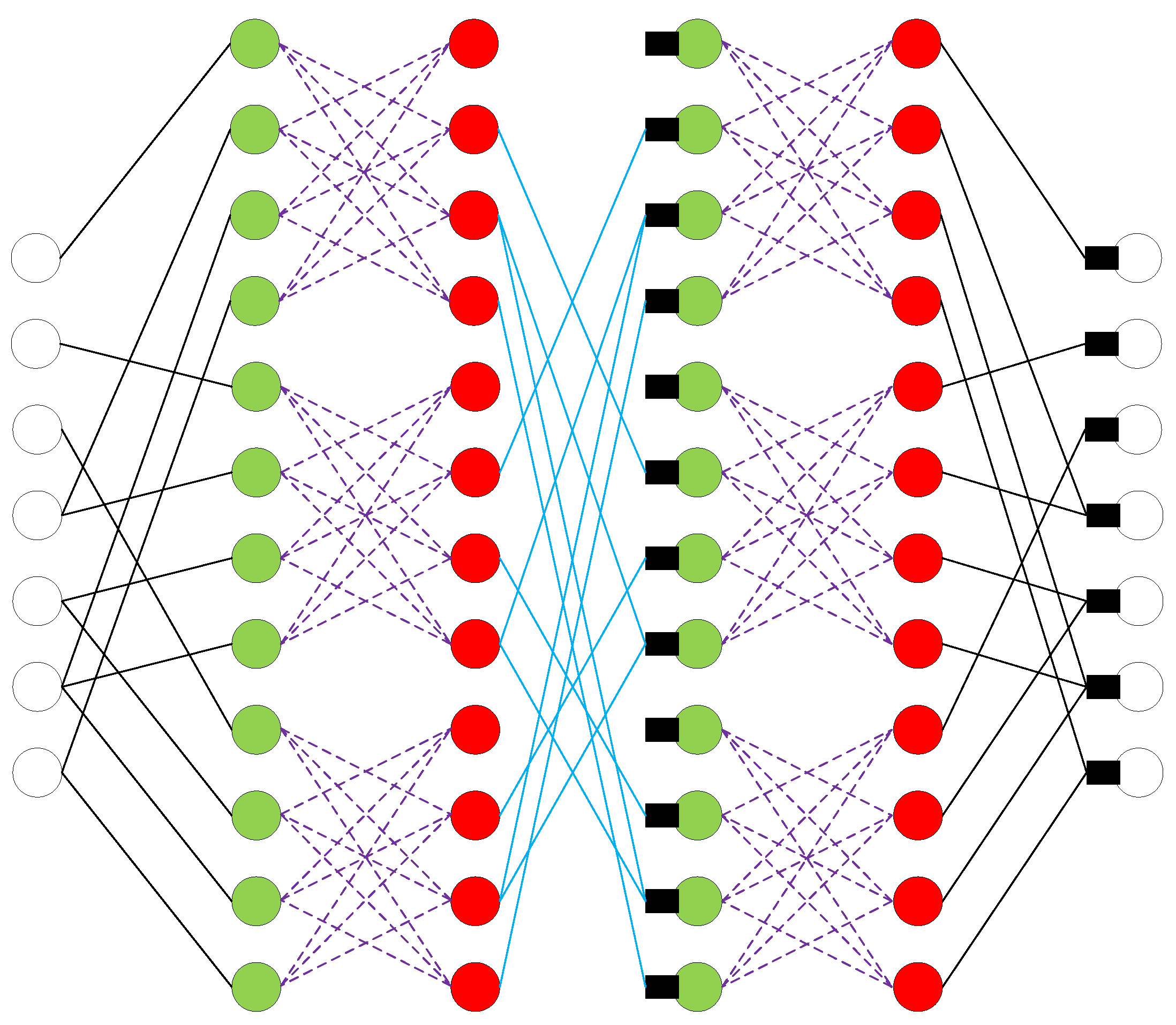
For neural networks, each layer represents a half-BP iteration (check nodes to variable nodes or variable nodes to check nodes). Therefore, it needs two layers (an odd layer and an even layer) to perform a single BP iteration. We denote the weights associated with each layer as
and
. Accordingly, (6) and (7) are replaced, respectively, by,
An example structure of constructed neural network for the (7,4) QR code is illustrated in
Figure 3.
By replacing BP decoders by min-sum decoders, we can obtain neural min-sum decoders as in (10). Here, we used a modified min-sum algorithm called threshold attenuated min-sum algorithm (TAMS) [
23], and the neural network version was given by,
where
and
are an attenuation coefficient and a threshold, respectively. The values of
and
were set empirically to 0.7 and 1.5, respectively. Moreover, a sigmoid function was applied to convert LLR to probabilities after the final iteration.
Given a parity check matrix, the network structure is determined. We applied the algorithm in [
21] to reduce the cycles in parity check matrices and used the cycle-reduced parity-check matrix to construct the neural network. We used different weights for
I times of BP/min-sum iterations, and the parameter space was
When all weights are set to 1, the neural BP/min-sum turns back to the original BP/min-sum algorithm.
To measure the difference between the output of network and the true codeword, we used the multiloss binary cross-entropy (BCE). Given iterations of
I and code length of
n, the neural network yielded output
, where
and
. The multiloss BCE between the true codeword
and the outputs
was calculated and accounted for the total loss after every BP/min-sum iteration as follows:
4. Cyclic mRRD
Trapping sets of small sizes can greatly influence the performance of BP or min-sum algorithms as shown in
Figure 4. The trapping sets were found by using the algorithm proposed in [
24].
Figure 4 and
Figure 5 show that the distribution of errors are more similar to the distribution of trapping sets rather than 4-cycles. That means trapping sets can also greatly affect the BP/min-sum performance for QR codes at high SNR such as LDPC codes, and the effect of short cycles become less important. Referring to
Figure 1, the mRRD chooses and applies a random permutation from
before each BP/min-sum decoder, which is equivalent to using a different parity check matrix for each BP/min-sum decoder. By permuting LLRs to other positions, the mRRD prevents nodes from receiving messages from the same group of neighboring nodes in the trapping sets or cycles and a falsely converged variable node may be corrected by the other nodes after the next BP decoder.
As we have analyzed before,
contains not only the cyclic shift, but also many other permutations for a cyclic code. The order of permutation groups for different QR codes are listed in
Table 1. We notice that the order of the permutation group of the (23,12) QR code is significantly larger than the others. That is because the permutation group of the (24,12) extended QR code contains two distinct groups of projective special linear (PSL) type, while the permutation groups of most other codes contain only one [
25]. Furthermore, the permutation group of the original code is composed by permutations which fix the overall check bit in the permutation group of the extended code.
Each permutation can be stored as a one-dimensional array using Cauchy’s two-line notation with the first line omitted. However, it still requires much memory to store those permutations. Alternatively, we can store the group generators only, which brings additional overheads at runtime to compute the composition of permutations. Furthermore, the implementation of a random permutation on circuits is complex when LLRs can be shuffled to any position. As a result, it needs multiple random swaps between LLR values to perform a single random permutation. Otherwise, we need a more complex design in order to shuffle LLRs in one step.
Cyclic shifts are easier to be implemented in hardware than random permutations. By shifting LLRs to their neighboring positions in a loop, any length of shift permutation can be easily implemented and rapidly performed. By using the same cyclic shift every time, the complexity of the implementation can be further reduced. Considering the above analysis, we can first compute the trapping set distribution
, where
is the number of trapping sets associated with node
. Then, we select a cyclic shift based on the distribution, that is, the bits associated with large numbers of trapping sets will be moved to the positions with less trapping sets. It allows zero overhead during the decoding process. The criterion to select good shifts from all cyclic shift permutations is proposed as Algorithm 1. After performing the algorithm, we can select the cyclic shift which has the highest score. If the algorithm returns multiple shifts with the same score, we choose the shift
that has the least length (i.e., is closest to 0 or
n). For example, suppose the algorithm returns 40 and 23 for the (47,24) QR code, implying that cyclic right shifts of 40 bits and 23 bits are both optimal. However, shifting right by 40 bits can be implemented as shifting left by 7, which is less than 23, so the final result is a cyclic shifting right by 40 bits.
| Algorithm 1 Criterion to find the best shift |
Input: Distribution of trapping sets: Output: The best shift: for to n do //Measure the change of the number of trapping sets for each bit. end for if then else end if |
The proposed method replaces the first random permutation by a random cyclic shift for each pipeline to give every pipeline a different starting point. After that, all the other random permutations in the original mRRD are replaced by a fixed right shift permutation. Since all permutations are replaced by cyclic shifts, we call the new modified mRRD Cyclic-mRRD. The Cyclic-mRRD is given in detail as Algorithm 2.
| Algorithm 2 Cyclic-mRRD |
Input: Cyclic right shift: , parity check matrix: code length: n, LLR vector: mRRD Size: Output: Decode results: for to W do for to L do if then //Rearrange bits to the original order //Append to success set break else //Record total shifted bits end if end for //Rearrange bits to the original order //Append to default set end for if then //No valid codewords, select from default set end if |
5. Simulation Results
The simulation and training were carried under BI-AWGN channels. All LLRs beyond were clipped to −20/+20. The training set contained vectors, which were all-zero codewords corrupted by random noises at = 3–5 dB, and the batch size was 200, whereas the BER and FER curves were obtained using randomly generated codewords and noises. We used the RMSProp optimizer in which the learning rate was set to 0.01. Other parameters were set to their default as per PyTorch’s implementation.
5.1. Neural BP/Min-Sum
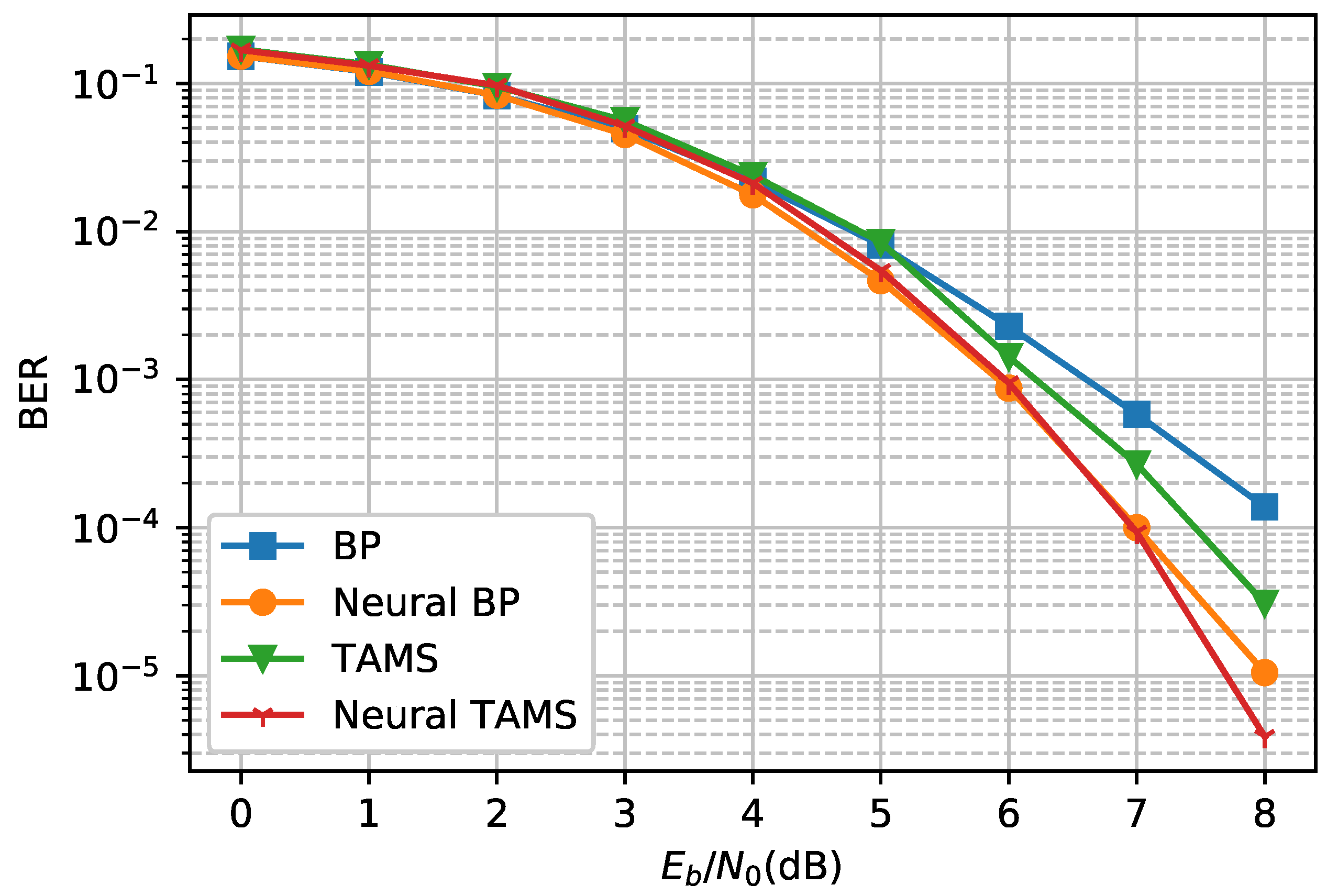
We first demonstrate the neural network versions of the BP and TAMS algorithms. As illustrated in
Figure 6, the neural network versions of the BP and TAMS algorithms both outperform the original BP/TAMS algorithm. The neural BP achieves a gain of 1.1 dB compared to BP when the BER is
. Neural TAMS has the best performance among these four decoders, and the gain is about 0.6 dB at a BER of
, when compared with the original TAMS algorithm. In addition, it has a relatively low complexity compared to the BP algorithm and neural BP. Therefore, we used neural TAMS as the default decoder in the following experiments.
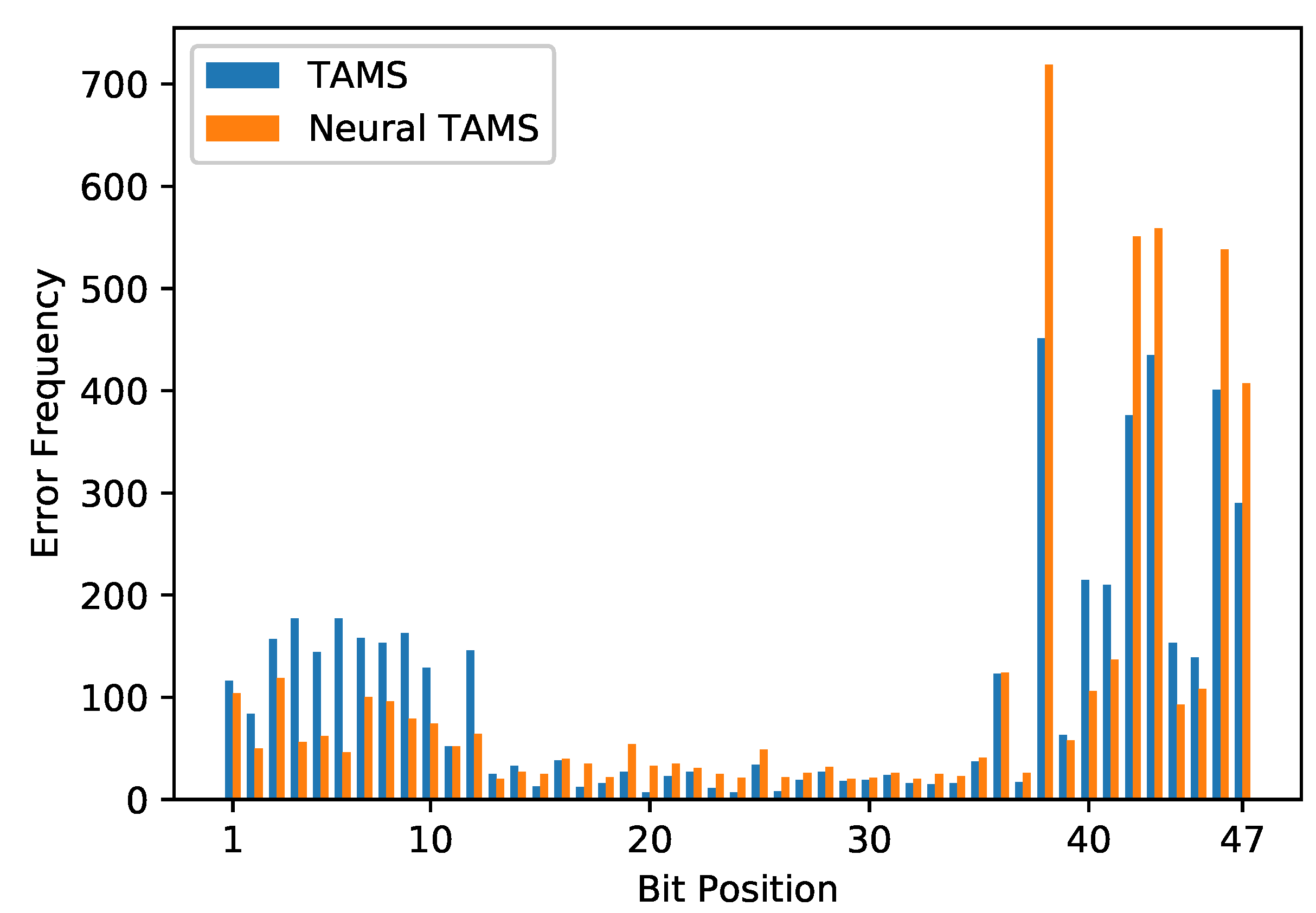
Figure 7 shows the error distributions of the TAMS algorithm and neural TAMS. The errors were counted until more than 5000 bit errors occurred. Though a neural network can mitigate the effect of trapping sets, the mitigation is limited, especially for those nodes which are involved in many trapping sets. So the error occurrences of these nodes become more dominant in a high-SNR regime.
5.2. Neural mRRD/Neural Cyclic-mRRD
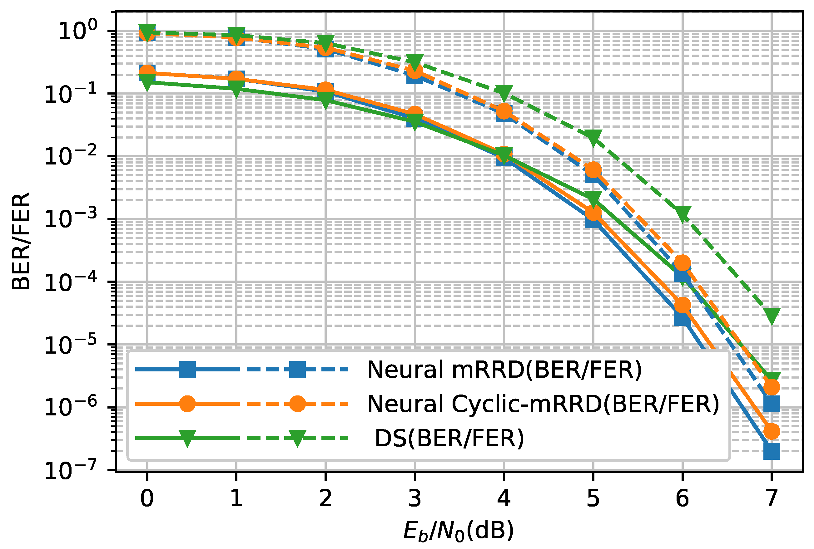
Figure 8,
Figure 9,
Figure 10 and
Figure 11 show the comparison on error performances of neural mRRD (5,10,5) and neural Cyclic-mRRD (5,10,5). The results were calculated after 100 frames errors had occurred and more than 1000 frames had been processed. The cyclic shifts were selected by using Algorithm 1 with trapping sets satisfying
.
Referring to
Figure 8, for the (47,24) QR code, the neural mRRD achieved a gain of 0.5 dB at BER
, compared with the DS algorithm. The neural Cyclic-mRRD had a slight loss of performance, which was about 0.08 dB at BER
, compared to neural mRRD, which randomly chooses permutations from the whole group. The selected cyclic right shift length was 22 based on Algorithm 1. We also observed that the FER of neural Cyclic-mRRD was lower than DS at all SNRs. However, at very low SNR, each incorrect mRRD/Cyclic-mRRD frame introduced additional bit errors compared to the DS algorithm.
Figure 9 shows the FER/BER performance of the neural mRRD and neural Cyclic-mRRD on the (71,36) QR code. The neural mRRD obtained a gain of about 1.0 dB at BER
compared to the DS algorithm. The selected cyclic shift for neural Cyclic-mRRD was a right shift of 36, and the loss of performance compared to the neural mRRD was about 0.3 dB at BER
.
Figure 10 shows the FER/BER performance of the neural mRRD and neural Cyclic-mRRD on the (73,37) QR code. The neural mRRD obtained a gain of about 0.5 dB at BER
compared to the DS algorithm. The selected cyclic shift for neural Cyclic-mRRD was a right shift of 31 bits. The performance loss compared to the neural mRRD was about 0.1 dB at BER
.
Figure 11 shows the FER/BER performance of the neural mRRD and neural Cyclic-mRRD on the (97,49) QR code. The neural mRRD obtained a gain of about 0.4 dB improvement at BER
compared to the DS algorithm. The selected cyclic shift for neural Cyclic-mRRD was a right shift of 31 bits. The performance loss compared to the neural mRRD was about 0.04 dB at BER
.
5.3. Longer QR Codes
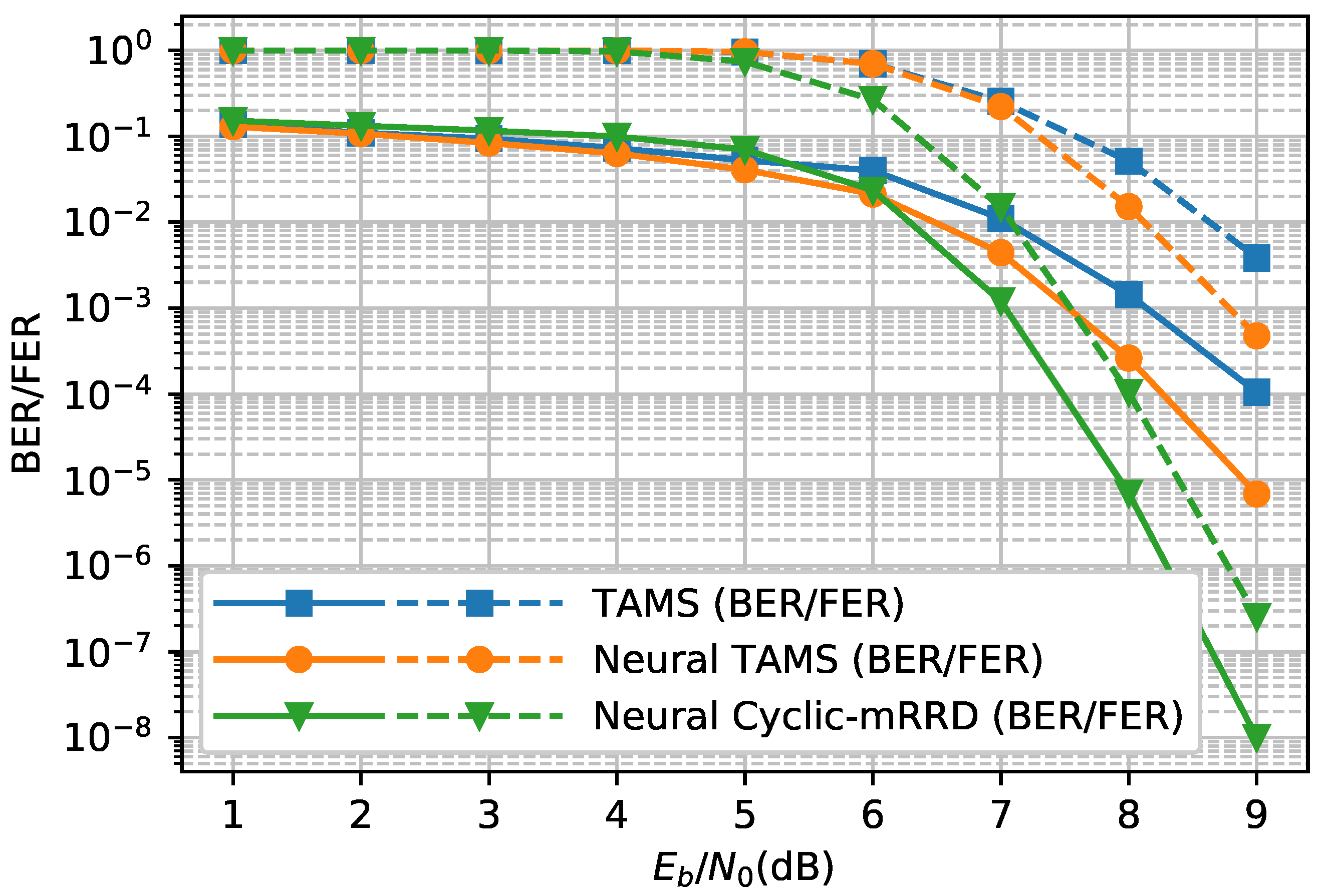
Note that we used a different set of hyperparameters to train the neural network for QR codes with code length more than 200. The training set contained
vectors which were corrupted by noises with SNR varying from 1 to 8 dB. The learning rate was set to 0.001, and the other hyperparameters remained the same. Furthermore, we used an ordinary BCE loss function instead of a multiloss BCE. We could not obtain the performance of the DS algorithm because the minimum distances of long QR codes are still unknown, and the complexity of the DS algorithm is very high for long QR codes. Neural TAMS and TAMS applied five iterations and Cyclic-mRRD’s size was (5,10,5).
Figure 12 shows the BER/FER performance of the neural mRRD and neural Cyclic-mRRD on the (241,121) QR code. The cyclic shift for neural Cyclic-mRRD was a right shift of 191 bits, which was selected by using trapping sets with
and
.
Figure 13 shows the BER/FER performance of the neural mRRD and neural Cyclic-mRRD on the (263,132) QR code. The cyclic shift was a right shift of 232 bits, which was selected by using trapping sets with
and
.
5.4. Complexity Analysis
The proposed Cyclic-mRRD method employs multiple BP/min-sum decoders and more multiplications on every iteration. However, most of them can run in parallel. Assume the number of edges in a Tanner graph is e. Each neural BP/min-sum iteration needs on average more multiplications than the original BP/min-sum iteration. However, the latency nearly remained the same because different nodes can process incoming messages simultaneously.
For the Cyclic-mRRD , it needs BP/min-sum iterations in the worst case, and iterations for the best case, because there are only I iterations to be performed for each pipeline in the best case. Considering that there are no data dependencies among different pipelines, W pipelines can decode the different shifted inputs at the same time. Then, the latency in the worst case reduces to iterations and I iterations for the best case. For our Cyclic-mRRD (5,10,5), the latency in parallel was 50 iterations in the worst case and 5 iterations in the best case.
It is hard to analyze the average complexity of the above decoders. Thus, the average time complexity at different SNRs was obtained by computing the average iterations needed to converge using 10,000 random frames, as shown in
Table 2. The legend “serial” means the sum of the number of min-sum iterations from all pipelines, and “parallel” denotes the largest number of iterations among all pipelines. The average serial/parallel iterations were calculated by summing up all iterations for each pipeline and divided by the number of codewords, which represents the time complexity when all pipelines run in serial. We can see that the average complexity of neural Cyclic-mRRD nearly achieved the best complexity at
(about 25 iterations in serial and 5 iterations in parallel), and the worst complexity at
(about 220 iterations in serial and 48 iterations in parallel).
6. Conclusions
In this paper, we proposed several neural-network-based methods to decode binary QR codes. We observed that the performance of the BP/min-sum algorithm was mainly affected by a small part of trapping sets, even though there were a huge number of four-cycles in the parity check matrix of QR codes. Based on this phenomenon, the proposed Cyclic-mRRD moved the nodes out from the trapping sets by using cyclic shifts. The simplification achieved similar performance as mRRD, while reducing the complexity of implementation and memory usage. Both the mRRD and Cyclic-mRRD outperformed the DS algorithm in terms of BER/FER performance, with less asymptotic time complexity.
Finally, we obtained the BER/FER performance of two longer QR codes using the proposed Cyclic-mRRD, though their error performances could not be determined without knowing their minimum distances.
Our future work will include approaching ML performance for longer QR codes with less or the same complexity. Furthermore, there are some possible improvements on the neural network, including training, data quantization and trapping set issues.

