Control Strategy and Corresponding Parameter Analysis of a Virtual Synchronous Generator Considering Frequency Stability of Wind Power Grid-Connected System

Abstract

The doubly-fed induction generator (DFIG) based on the control strategy of constant parameter virtual synchronous generator (VSG) can cause problems of sharp frequency variations in the grid-connected system, long adjustment times, and large overshoot of the active power output from the DFIG. Aiming at dealing with the above-mentioned problems, a VSG control strategy with an independent flexible link (IFLVSG) is proposed in this paper without changing the parameters and structure of the VSG, so that the moment of inertia and damping coefficient can be flexibly adjusted according to the change of the system frequency, so as to improve the system frequency stability. To form a complete selection scheme for control parameters in IFL, the state space equation including IFLVSG control is established, and the advantages of exponential IFL are highlighted by using the sensitivity calculation method. At the same time, in order to improve the analysis efficiency, the main control parameters affecting the frequency stability of the system are selected according to the sensitivity value. Finally, the root locus analysis method is used to reveal the influence law of the main control parameters on the frequency stability of the system. The formed scheme provides a theoretical basis for the selection of control parameters.

1. Introduction

Currently, traditional fossil energy sources are becoming increasingly depleted and bring a series of pollution problems [1]. Wind power, as a clean energy source, has been developing rapidly [2,3]. The grid-connected control strategy of the DFIG in the wind power generation system is usually based on a constant power vector control strategy, resulting in a complete decoupling of the DFIG output power from the frequency of the grid-connected system. It makes the DFIG unable to respond to frequency disturbances (i.e., load variations or generator output power variations) that occur in the system, which will have an extremely negative impact on the stability of the system frequency [4,5]. To enable the DFIG to have the same frequency support capability for the grid-connected system as the synchronous generator, scholars have introduced the VSG control strategy into DFIG’s converters, aiming to enable the DFIG to have the same inertia and frequency adjustment characteristics as the synchronous generator [6,7,8]. However, the moment of inertia and damping coefficient in the VSG control strategy have a great impact on the frequency stability of the system [9]. Therefore, it is necessary and feasible to improve the frequency stability of the system by adjusting the moment of inertia and damping coefficient.

To improve the stability of the frequency of distributed generation systems, reference [10] proposed a bang-bang control strategy, i.e., the moment of inertia varies between two fixed values. When the variation of the system frequency is less than the set threshold, the moment of inertia takes a smaller value, otherwise, it takes a larger value. Overall, the bang-bang control strategy improves the frequency stability of the system compared to the VSG control strategy, but it has suffered the defect of having too small a range of the moment of inertia. Different flexible moment of inertia control strategies were used to improve the response characteristics of the system frequency in [11,12,13], but the advantages and disadvantages of the control strategies used were not highlighted. In reference [14], a fuzzy control strategy was introduced to the VSG control strategy to effectively reduce the maximum amplitude of the system frequency variation and thus prevent the out-of-limit of the frequency. In reference [15], a dual flexible moment of inertia control strategy was proposed and a balance between power adjustment and frequency adjustment was achieved according to different operating conditions. Compared with the constant moment of inertia, the above-mentioned reference can attenuate the sharp variations in system frequency to a certain extent through real-time flexible adjustment of the moment of inertia.

To overcome the adverse effects of fixed parameters of the VSG control strategy, references [16,17] reveal the relationship between the moment of inertia and the damping coefficient with the damping ratio, dynamic characteristics, and stability of the system, and suppresses the power overshoot and shortens the adjustment time by flexibly adjusting the damping coefficient. Compared with [16,17], reference [18] utilized a radial basis function (RBF) to adjust the moment of inertia in real time based on the analysis of the effect of the moment of inertia on the dynamic performance of the system, and the damping coefficient was flexibly adjusted to further suppress the power oscillation. However, the operation time of the adopted method may be longer, owing to the complex network structure of the RBF and the large number of hidden layer neurons. In reference [19], a flexible moment of inertia and damping coefficient were designed with the objective of maintaining the optimum damping ratio of the system. However, the designed flexible moment of inertia and damping coefficient can only be selected between small and large values. Reference [20] divided the frequency variation curve of the system during transients into several intervals and designed the corresponding flexible moment of inertia and damping coefficient according to the role they played in the different intervals.

However, although a flexible moment of inertia and a damping coefficient have been constructed in the above references, the influence of their control parameters on the frequency stability of the system remains unclear, resulting in a lack of basis for the selection of control parameters. In this paper, an exponential IFLVSG control strategy is proposed to improve the frequency stability of the system without changing the structure and parameters of the VSG control strategy. Moreover, a state space equation is innovatively established to include all the parameters of the IFLVSG control strategy and the grid-connected line. The sensitivity calculation method used in this paper not only clarifies the superiority of the proposed exponential IFLVSG control strategy but also selects the main control parameters affecting the system frequency stability, thus avoiding in-depth analysis of insignificant parameters and greatly improving the analysis efficiency. The root locus analysis reveals the influence law of the main control parameters on the frequency stability of the system, which provides a basis for the selection of control parameters.

The rest of this paper is organized as follows. Section 2 establishes the mathematical models of the DFIG and IFLVSG control strategies. Section 3 is based on the relationship between IFL and system frequency stability, three typical IFLVSG control strategies are established. In Section 4, the sensitivity of the parameters and its influence on the frequency stability of the system are analyzed. The superiority of the exponential IFLVSG control strategy and the effectiveness of the parameter selection scheme are verified in Section 5. Finally, this paper is concluded in Section 6.

2. Mathematical Modeling of DFIG and IFLVSG Control Strategy

To enable the DFIG to obtain similar output power characteristics as a synchronous generator, the DFIG’s rotor side converter (RSC) uses a dual closed-loop control strategy with the IFLVSG control strategy as the outer loop and the rotor current control strategy as the inner loop.

2.1. Mathematical Model of the DFIG

To obtain the control equations for the DFIG rotor voltage, the stator voltage is set in the dq coordinate system. Let the d axis as the vector direction of the oriented voltage, the voltage equation and flux linkage equation for the stator and rotor can be expressed as follows [16]:

$$\left\{\begin{array}{l}{u}_{sd}=R_s{i}_{sd}+\frac{\mathrm{d}{\psi }_{sd}}{\mathrm{d}t}-{\omega }_s{\psi }_{sq}\\ u_{sq}=R_s{i}_{sq}+\frac{\mathrm{d}{\psi }_{sq}}{\mathrm{d}t}+{\omega }_s{\psi }_{sd}\\ u_{rd}=R_r{i}_{rd}+\frac{\mathrm{d}{\psi }_{rd}}{\mathrm{d}t}-{\omega }_{sl1}{\psi }_{rq}\\ u_{rq}=R_r{i}_{rq}+\frac{\mathrm{d}{\psi }_{rq}}{\mathrm{d}t}+{\omega }_{sl1}{\psi }_{rd}\end{array}\right.$$

(1)

$$\left\{\begin{array}{l}{\psi }_{sd}=L_s{i}_{sd}+L_m{i}_{rd}\\ {\psi }_{sq}=L_s{i}_{sq}+L_m{i}_{rq}\\ {\psi }_{rd}=L_m{i}_{sd}+L_r{i}_{rd}\\ {\psi }_{rq}=L_m{i}_{sq}+L_r{i}_{rq}\end{array}\right.$$

(2)

where $u_{sd}$, $u_{sq}$, $u_{rd}$, and $u_{rq}$ are the voltages of the stator and rotor in the dq axis, respectively. $R_s$ and $R_r$ are the resistances of the stator and rotor windings, respectively. ${\omega }_{sl1}$ is the angular slip velocity, i.e., ${\omega }_{sl1}$ = ${\omega }_s$ − ${\omega }_r$, ${\omega }_s$ and ${\omega }_r$ are the stator and rotor angular velocities, respectively. $i_{sd}$, $i_{sq}$, $i_{rd}$, and $i_{rq}$ are the currents of the stator and rotor in the dq axis, respectively. ${\psi }_{sd}$, ${\psi }_{sq}$, ${\psi }_{rd}$, and ${\psi }_{rq}$ are the flux linkages of the stator and rotor in the dq axis, respectively. $L_s$ and $L_r$ are the self-inductance of the stator and rotor windings, respectively. $L_m$ is the mutual inductance between the stator and rotor windings. Combining Equations (1) and (2) yields the following equation [21]:

$$\left\{\begin{array}{l}{u}_{rd}=R_r{i}_{rd}+\sigma L_r\frac{\mathrm{d}{i}_{rd}}{\mathrm{d}t}-{\omega }_{sl1}\sigma L_r{i}_{rq}\\ u_{rq}=R_r{i}_{rq}+\sigma L_r\frac{\mathrm{d}{i}_{rq}}{\mathrm{d}t}+{\omega }_{sl1}(\frac{L_m^2}{L_s}{i}_{ms}+\sigma L_r{i}_{rd})\end{array}\right.$$

(3)

where the leakage coefficient $\sigma =\left(L_s{L}_r-L_m^2\right)/\left(L_s{L}_r\right)$, and $i_{ms}$ is the equivalent excitation current of the stator. A feedforward compensation control strategy is adopted for the cross-coupling terms generated in the dq axis, and a proportional-integral (PI) controller is introduced. The equation for direct control of rotor voltage from rotor current is as follows [21]:

$$\left\{\begin{array}{l}{u}_{rdc}=(K_{pd}+\frac{K_{id}}{s})(i_{rd\_ref}-i_{rd})-{\omega }_{sl1}\sigma L_r{i}_{rq}\\ u_{rqc}=(K_{pq}+\frac{K_{iq}}{s})(i_{rq\_ref}-i_{rq})+{\omega }_{sl1}(\frac{L_m^2}{L_s}{i}_{ms}+\sigma L_r{i}_{rd})\end{array}\right.$$

(4)

where $K_{pd}$, $K_{pq}$, $K_{id}$, and $K_{iq}$ are the regulation coefficients in the PI controller. $i_{rd\_ref}$ and $i_{rq\_ref}$ are reference values of the rotor current in the dq axis, respectively. $u_{rdc}$ and $u_{rqc}$ are the components of rotor voltage control equation in the dq axis, respectively.

As the IFLVSG control strategy is introduced into the RSC in this paper, and the grid side converter (GSC) uses the more common dual closed-loop control strategy with outer DC bus voltage loop and inner current loop, the control strategy of the GSC is not described in detail.

2.2. Mathematical Model of the VSG Control Strategy

The VSG control strategy is divided into an active power-frequency loop and a reactive power-voltage loop. When the number of pole-pairs n = 1, the active power-frequency loop is expressed as follows based on the rotor equation of motion of a synchronous generator [6]:

$$\left\{\begin{array}{l}\frac{P_0-P_e}{{\omega }_0}-D_{p0}(\omega -{\omega }_0)=J_0\cdot \mathrm{d}(\omega -{\omega }_0)/\mathrm{d}t\\ \frac{\mathrm{d}\theta }{\mathrm{d}t}=\omega \end{array}\right.$$

(5)

where the active power $P_e$ output from the DFIG is used as the electromagnetic power for the VSG control strategy, $J_0$ and $D_{p0}$ are the moment of inertia and damping coefficient, respectively. ${\omega }_0$ and ω are the rated angular velocity and the angular velocity generated by the active power-frequency loop, respectively. θ is the generated phase. Notably, this paper applies the overspeed operation method to correct the maximum power curve in the original maximum power point tracking (MPPT) controller, resulting in a corrected maximum power point tracking controller as MPPT-MAR, which allows the DFIG to obtain an active power margin [22]. When the rotor speed ${\omega }_r$ passes through the MPPT-MAR controller, the active power command value $P_0$ is obtained.

According to the excitation voltage regulation equation of the synchronous generator, the reactive power-voltage loop is expressed as follows:

$$E=E_0+(Q_0-Q_e)(K_{pQ}+\frac{K_{iQ}}{s})\frac{1}{T_{a}s+1}$$

(6)

where $E_0$ and E are the amplitude of the set rated voltage and the amplitude of the generated internal potential, respectively. $Q_0$ is the set reactive power reference value. The reactive power $Q_e$ output is used by the DFIG as the reactive power input of VSG control strategy. $K_{pQ}$ and $K_{iQ}$ are the proportional and integral coefficients in the reactive power-voltage loop, respectively. $T_a$ is the time constant of the delay link. Notably, the expressions and parameters of the reactive power-voltage loop in the IFLVSG control strategy are the same as in Equation (6).

2.3. Mathematical Model of the IFLVSG Control Strategy

In this paper, without changing the VSG control strategy, IFL, which is related to the system frequency deviation, is introduced to further improve the stability of the system frequency. Based on the deviation of the system frequency and its differential of deviation, the IFL produces a frequency modulation power P_IFL as follows:

$$P_{\mathrm{IFL}}=-K_{\mathrm{IFLp}}(\omega -{\omega }_0)-K_{\mathrm{IFLd}}\cdot \mathrm{d}(\omega -{\omega }_0)/\mathrm{d}t$$

(7)

where $K_{\mathrm{IFLp}}$ and $K_{\mathrm{IFLd}}$ are the proportional and differential coefficients in IFL, respectively, and their specific expressions are given in Section 3. $P_{\mathrm{IFL}}$ and $P_0$ form the new virtual mechanical input power $P_{m\_new}$ as follows:

$$P_{m\_new}=P_0+P_{\mathrm{IFL}}$$

(8)

The active power-frequency loop expression for the IFLVSG control strategy obtained from Equation (9) is as follows:

$$\left\{\begin{array}{l}\frac{P_{m\_new}-P_e}{{\omega }_0}-D_{p0}(\omega -{\omega }_0)=J_0\cdot \mathrm{d}(\omega -{\omega }_0)/\mathrm{d}t\\ \frac{\mathrm{d}\theta }{\mathrm{d}t}=\omega \end{array}\right.$$

(9)

The meaning of the parameters in Equation (9) is the same as in Equation (5).

3. Analysis of IFLVSG Control Strategy

3.1. Control Structure of a DFIG-IFLVSG Grid-Connected System

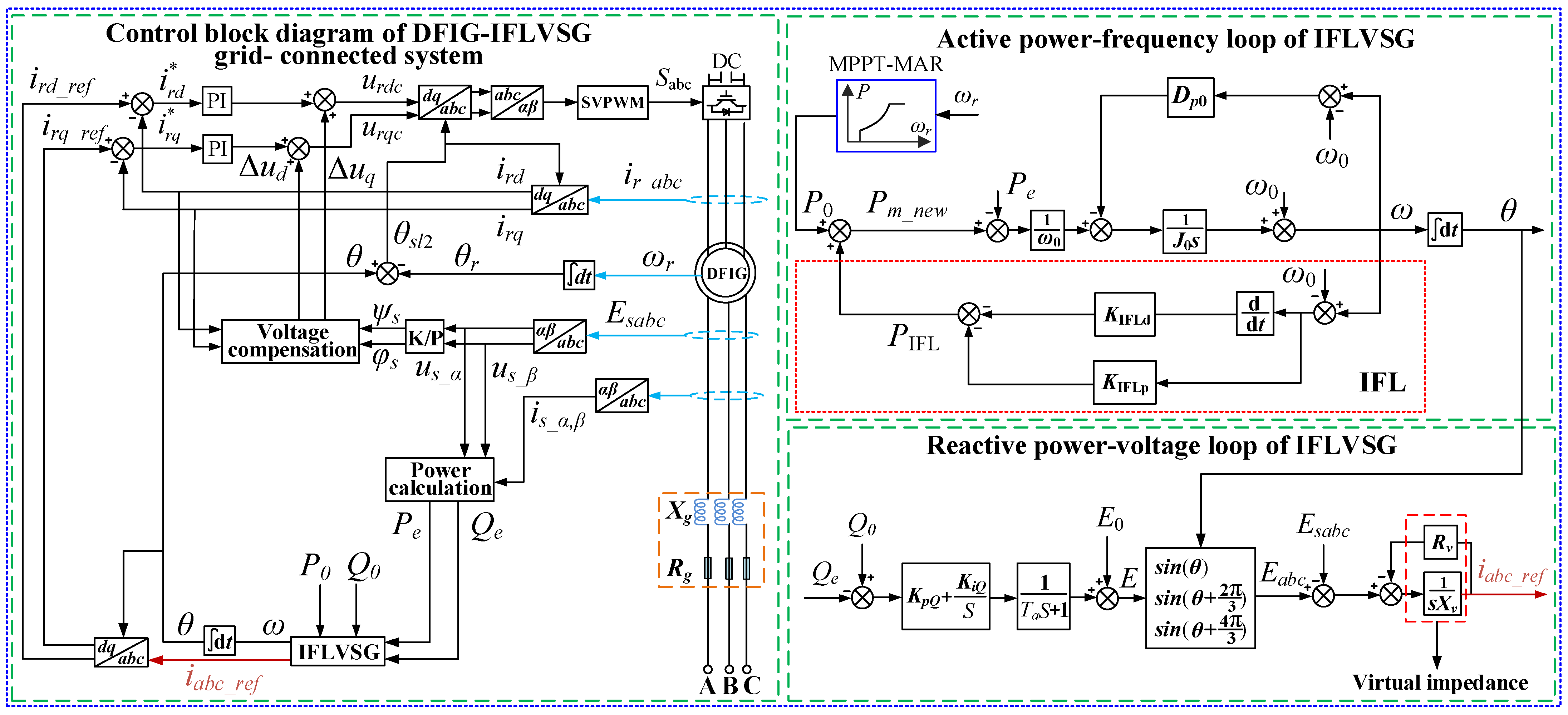
Based on the mathematical model in Section 2, this paper proposes a double closed-loop control strategy with IFLVSG as the outer loop and rotor current as the inner loop, and the control structure of the DFIG-IFLVSG grid-connected system is shown in Figure 1. The virtual current $i_{abc\_ref}$ output from the reactive power-voltage loop in the IFLVSG control strategy in Figure 1 serves as the reference current of the inner loop of rotor current. $i_{rd\_ref}$ and $i_{rq\_ref}$ are the reference values of the rotor current components in the dq axis, $i_{r\_abc}$ is the rotor current, $i_{rd}$ and $i_{rq}$ are the rotor current components in the dq axis. $i_{rd}^{*}$ and $i_{rq}^{*}$ are the difference between the reference values of the rotor current and rotor current in the dq axis, respectively. Δu_d and Δu_q are the compensation terms for the rotor voltage component in the dq axis. ${\omega }_r$, ${\theta }_r$, ${\phi }_s$, and ${\psi }_s$ are the rotor angular velocity, rotor phase, stator voltage phase, and flux linkage, respectively, ω and θ are the angular velocity and phase output from the IFLVSG control strategy, respectively, ${\theta }_{sl2}$ is the slip phase, i.e., ${\theta }_{sl2}=\theta -{\theta }_r$. $E_{sabc}$ and E are the stator voltage and the internal potential amplitude generated by the IFLVSG control strategy, respectively. θ and E form the internal potential $E_{abc}$ generated by the IFLVSG control strategy. $R_g$ and $X_g$ are the line resistance and inductive reactance, respectively, $R_v$ and $X_v$ are the virtual resistance and inductive reactance, respectively.

The K/P in Figure 1 represents the conversion from a rectangular coordinate system to a polar coordinate system with the stator flux linkage and voltage compensation expressions as follows:

$$\left\{\begin{array}{l}{\psi }_s=\frac{\sqrt{u_{s\_\alpha }^2+u_{s\_\beta }^2}}{{\omega }_0}\\ {\phi }_s=arctan\frac{u_{s\_\alpha }}{u_{s\_\beta }}-\frac{\pi }{2}\end{array}\right.$$

(10)

$$\left\{\begin{array}{l}\Delta u_d={\omega }_{sl2}\sigma L_r{i}_{rd}+{\omega }_{sl2}\frac{L_m^2}{L_s}{i}_{ms}\\ \Delta u_q=-{\omega }_{sl2}\sigma L_r{i}_{rq}\end{array}\right.$$

(11)

where ${\omega }_{sl2}$ is the angular slip velocity generated based on the IFLVSG control strategy, i.e., ${\omega }_{sl2}=\omega -{\omega }_r$. $u_{s\_\alpha }$ and $u_{s\_\beta }$ are the components of the stator voltage in the αβ axis, respectively.

3.2. Control Principle of IFL

According to Equation (5), the angular velocity deviation Δω and the change rate of the angular velocity deviation $\mathrm{d}\Delta \omega /\mathrm{d}t$ based on the VSG control strategy are derived as follows:

$$\mathrm{d}\Delta \omega /\mathrm{d}t=\frac{P_0-P_e-(D_{p0}{\omega }_0)\Delta \omega }{J_0}$$

(12)

$$\Delta \omega =\frac{P_0-P_e-J_0\left(\mathrm{d}\Delta \omega /\mathrm{d}t\right)}{D_{p0}{\omega }_0}$$

(13)

As shown in Equation (12), assuming that $P_0-P_e-\left(D_{p0}{\omega }_0\right)\Delta \omega$ remains constant, $\mathrm{d}\Delta \omega /\mathrm{d}t$ decreases as $J_0$ increases, which prevents the rate of frequency variation from being too fast. As shown in Equation (13), assuming that $P_0-P_e-J_0\left(\mathrm{d}\Delta \omega /\mathrm{d}t\right)$ remains constant, Δω decreases as $D_{p0}$ increases, which prevents excessive frequency deviation.

The $\mathrm{d}\Delta \omega /\mathrm{d}t$ and Δω based on the IFLVSG control strategy obtained from Equations (7)–(9) are as follows:

$$\mathrm{d}\Delta \omega /\mathrm{d}t=\frac{P_0-P_e-(K_{\mathrm{IFLp}}+D_{p0}{\omega }_0)\Delta \omega }{J_0+K_{\mathrm{IFLd}}}$$

(14)

$$\Delta \omega =\frac{P_0-P_e-(J_0+K_{\mathrm{IFLd}})(\mathrm{d}\Delta \omega /\mathrm{d}t)}{K_{\mathrm{IFLp}}+D_{p0}{\omega }_0}$$

(15)

As shown from the comparisons between Equations (12) and (14), (13), and (15); Equations (7) and (8); and the results of above analyses, the introduced IFL can further suppress dΔω/dt and Δω without changing the structure and parameters of the VSG control strategy.

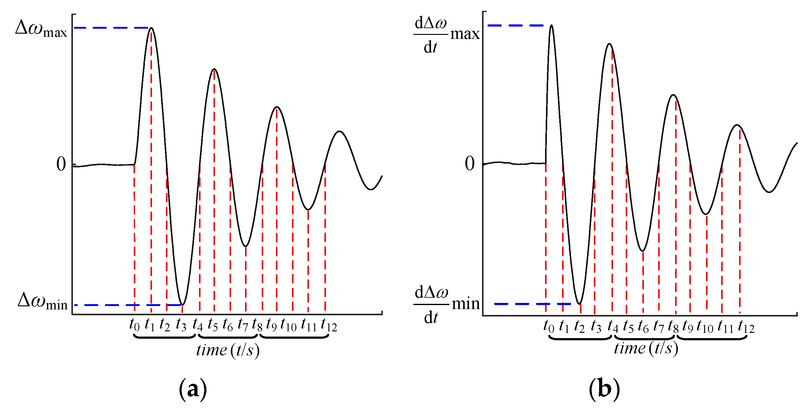
Since a change in wind speed causes a change in ${\omega }_r$, leading to a change in $P_0$, the oscillation curves of $\mathrm{d}\Delta \omega /\mathrm{d}t$ and Δω during the change are divided into multiple intervals with reference to [20], where $t_0-t_4$, $t_4-t_8$, $t_8-t_{12}$ correspond to one oscillation period, and in each oscillation period, Δω and $\mathrm{d}\Delta \omega /\mathrm{d}t$ are divided into four intervals, as shown in Figure 2. Since Δω and $\mathrm{d}\Delta \omega /\mathrm{d}t$ in the three oscillation periods of $t_0-t_4$, $t_4-t_8$, $t_8-t_{12}$ are consistent, only four intervals in the period t₀ − t₄ are analyzed below.

In the first interval ($t_0-t_1$) and the third interval ($t_2-t_3$), since Δω and $\mathrm{d}\Delta \omega /\mathrm{d}t$ change in the same direction, $K_{\mathrm{IFLd}}$ is needed to further constrain $\mathrm{d}\Delta \omega /\mathrm{d}t$, thus preventing further increases in Δω and the premature reach of the maximum amplitude of the frequency deviation $\Delta {\omega }_{\mathrm{AMP}}$, and suppressing sharp variations in frequency. However, increasing $K_{\mathrm{IFLp}}$ reduces Δω, but leads to the premature reach of $\Delta {\omega }_{\mathrm{AMP}}$ [9]. Therefore, the main purpose of the first and third intervals is to allow $K_{\mathrm{IFLd}}$ to participate in the adjustment of the system frequency, with $K_{\mathrm{IFLp}}$ remaining unchanged.

In the second interval ($t_1-t_2$) and the fourth interval ($t_3-t_4$), since Δω and $\mathrm{d}\Delta \omega /\mathrm{d}t$ change in the opposite direction, if $K_{\mathrm{IFLd}}$ is involved in the adjustment of the system frequency, it will suppress $\mathrm{d}\Delta \omega /\mathrm{d}t$, which has a detrimental effect on the recovery of Δω. Therefore, it is not appropriate for $K_{\mathrm{IFLd}}$ to participate in system frequency adjustment in these two intervals. Since $K_{\mathrm{IFLp}}$ is able to reduce Δω, the main purpose of the second and fourth intervals is to allow $K_{\mathrm{IFLp}}$ to participate in system frequency adjustment, with $K_{\mathrm{IFLd}}$ remaining unchanged. The specific selection rules for $K_{\mathrm{IFLp}}$ and $K_{\mathrm{IFLd}}$ are shown in

Table 1. Selection rules for K_IFLd and K_IFLp.

Interval	Δω·dΔω/dt	KIFLd	KIFLp
1	>0	increase	constant
2	<0	constant	increase
3	>0	increase	constant
4	<0	constant	increase

.

Since the role of $K_{\mathrm{IFLp}}$ and $K_{\mathrm{IFLd}}$ in the oscillation process is consistent in each interval, whether it is a complete oscillation period or multiple complete oscillation periods, or if a complete period is not satisfied, $K_{\mathrm{IFLp}}$ and $K_{\mathrm{IFLd}}$ are referred to the selection rules of Table 1.

The IFLVSG control strategy proposed in this paper is derived from the selection rules in Table 1. $K_{\mathrm{IFLd}}$ is constructed as a function of $\mathrm{d}\Delta \omega /\mathrm{d}t$, while $K_{\mathrm{IFLp}}$ is constructed as a function of Δω. At this point, $K_{\mathrm{IFLd}}$ and $K_{\mathrm{IFLp}}$ can be adjusted according to the real time $\mathrm{d}\Delta \omega /\mathrm{d}t$ and Δω, respectively. As both $K_{\mathrm{IFLd}}$ and $K_{\mathrm{IFLp}}$ can be flexibly adjusted, the following three expressions for $K_{\mathrm{IFLd}}$ and $K_{\mathrm{IFLp}}$ are investigated to better enhance the stability of the system frequency.

3.2.1. $K_{\mathrm{IFLd}}$ and $K_{\mathrm{IFLp}}$ Based on the Bang-Bang Control Strategy

Based on the bang-bang control strategy proposed in reference [10], the expressions for $K_{\mathrm{IFLd}}$ and $K_{\mathrm{IFLp}}$ are as follows:

$$K_{\mathrm{IFLd}}=\left\{\begin{array}{l}0\Delta \omega \cdot (\mathrm{d}\Delta \omega /\mathrm{d}t)<0\\ M_1\Delta \omega \cdot (\mathrm{d}\Delta \omega /\mathrm{d}t)>0\cap \left|\mathrm{d}\Delta \omega /\mathrm{d}t\right|>T_{\mathrm{j}}\cap \left|\Delta P_c\right|>P_{\mathrm{j}}\end{array}\right.$$

(16)

$$K_{\mathrm{IFLp}}=\left\{\begin{array}{l}0\Delta \omega \cdot (\mathrm{d}\Delta \omega /\mathrm{d}t)>0\\ W_1\Delta \omega \cdot (\mathrm{d}\Delta \omega /\mathrm{d}t)<0\cap \left|\Delta \omega \right|>T_{\mathrm{d}}\cap \left|\Delta P_c\right|>P_{\mathrm{j}}\end{array}\right.$$

(17)

where $T_{\mathrm{j}}$ is the threshold of $\left|\mathrm{d}\Delta \omega /\mathrm{d}t\right|$ with $T_{\mathrm{j}}>0$, $T_{\mathrm{d}}$ is the threshold of $\left|\Delta \omega \right|$ with $T_{\mathrm{d}}>0$. $\left|\Delta P_c\right|$ is the absolute value of the change in $P_e$ and $P_{\mathrm{j}}$ is the threshold of $\left|\Delta P_c\right|$.

3.2.2. Arctangent $K_{\mathrm{IFLd}}$ and $K_{\mathrm{IFLp}}$

$K_{\mathrm{IFLd}}$ and $K_{\mathrm{IFLp}}$ can select arctan functions with upper and lower bounds so that $K_{\mathrm{IFLd}}$ and $K_{\mathrm{IFLp}}$ can vary within a certain range. In this case, the expressions for $K_{\mathrm{IFLd}}$ and $K_{\mathrm{IFLp}}$ are as follows:

$$K_{\mathrm{IFLd}}=\left\{\begin{array}{l}0\Delta \omega \cdot (\mathrm{d}\Delta \omega /\mathrm{d}t)<0\\ M_{2}arctan\left|\mathrm{d}\Delta \omega /\mathrm{d}t\right|\Delta \omega \cdot (\mathrm{d}\Delta \omega /\mathrm{d}t)>0\cap \left|\mathrm{d}\Delta \omega /\mathrm{d}t\right|>T_{\mathrm{j}}\cap \left|\Delta P_c\right|>P_{\mathrm{j}}\end{array}\right.$$

(18)

$$K_{\mathrm{IFLp}}=\left\{\begin{array}{l}0\Delta \omega \cdot (\mathrm{d}\Delta \omega /\mathrm{d}t)>0\\ W_{2}arctan\left|\Delta \omega \right|\Delta \omega \cdot (\mathrm{d}\Delta \omega /\mathrm{d}t)<0\cap \left|\Delta \omega \right|>T_{\mathrm{d}}\cap \left|\Delta P_c\right|>P_{\mathrm{j}}\end{array}\right.$$

(19)

where $M_2$ is the control parameter in the arctangent $K_{\mathrm{IFLd}}$ and $W_2$ is the control parameter in the arctangent $K_{\mathrm{IFLp}}$. When $\mathrm{d}\Delta \omega /\mathrm{d}t$, Δω, and $\Delta P_c$ all exceed the set threshold values, $K_{\mathrm{IFLd}}$ and $K_{\mathrm{IFLp}}$ are flexibly adjusted in real time according to $\mathrm{d}\Delta \omega /\mathrm{d}t$ and Δω respectively in the form of arctangent functions, thus improving the stability of the system frequency.

3.2.3. Exponential $K_{\mathrm{IFLd}}$ and $K_{\mathrm{IFLp}}$

A monotonically increasing exponential $K_{\mathrm{IFLd}}$ and $K_{\mathrm{IFLp}}$ is proposed so that they can vary in the form of exponential functions. In this case, the expressions for $K_{\mathrm{IFLd}}$ and $K_{\mathrm{IFLp}}$ are as follows:

$$K_{\mathrm{IFLd}}=\left\{\begin{array}{l}0\Delta \omega \cdot (\mathrm{d}\Delta \omega /\mathrm{d}t)<0\\ M_3{\left|\mathrm{d}\Delta \omega /\mathrm{d}t\right|}^{M_4}\Delta \omega \cdot (\mathrm{d}\Delta \omega /\mathrm{d}t)>0\cap \left|\mathrm{d}\Delta \omega /\mathrm{d}t\right|>T_{\mathrm{j}}\cap \left|\Delta P_c\right|>P_{\mathrm{j}}\end{array}\right.$$

(20)

$$K_{\mathrm{IFLp}}=\left\{\begin{array}{l}0\Delta \omega \cdot (\mathrm{d}\Delta \omega /\mathrm{d}t)>0\\ W_3{\left|\Delta \omega \right|}^{W_4}\Delta \omega \cdot (\mathrm{d}\Delta \omega /\mathrm{d}t)<0\cap \left|\Delta \omega \right|>T_{\mathrm{d}}\cap \left|\Delta P_c\right|>P_{\mathrm{j}}\end{array}\right.$$

(21)

where $M_3$ and $M_4$ are the control parameters in the exponential $K_{\mathrm{IFLd}}$, while $W_3$ and $W_4$ are the control parameters in the exponential $K_{\mathrm{IFLp}}$. $K_{\mathrm{IFLd}}$ and $K_{\mathrm{IFLp}}$ are flexibly adjusted in real time according to $\mathrm{d}\Delta \omega /\mathrm{d}t$ and Δω in the form of exponential functions, thus suppressing $\mathrm{d}\Delta \omega /\mathrm{d}t$ and Δω. It can be seen from Equations (20) and (21) that both exponential $K_{\mathrm{IFLd}}$ and $K_{\mathrm{IFLp}}$ contain two control parameters, so that $K_{\mathrm{IFLd}}$ and $K_{\mathrm{IFLp}}$ can be determined by two control parameters, instead of only one control parameter as in Equations (18) and (19), thus eliminating the hidden danger that a single control parameter has too great an influence on the system. In addition, $\mathrm{d}\Delta \omega /\mathrm{d}t$ in Equation (20) and Δω in Equation (21) are equivalent to the base of the exponential function. Based on the characteristics of the exponential function, when $\mathrm{d}\Delta \omega /\mathrm{d}t$ or Δω is large, $K_{\mathrm{IFLd}}$ and $K_{\mathrm{IFLp}}$ can rapidly increase to quickly suppress the oscillation of the system frequency and reduce the maximum deviation between the system frequency and the rated frequency.

4. Sensitivity Analysis of Control Parameters and Its Influence on Frequency Stability

4.1. Small-Signal Model of the DFIG-IFLVSG Grid-Connected System

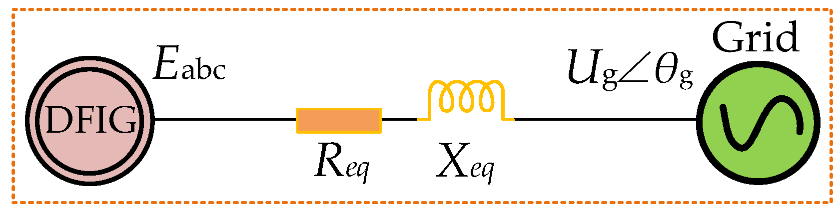
The equivalent circuit diagram of the DFIG-IFLVSG grid-connected system is established, as shown in Figure 3. $R_{eq}$ and $X_{eq}$ are the sum of system resistance and inductive resistance, i.e., $R_{eq}=R_g+R_v$, and $X_{eq}=X_g+X_v$. $U_{\mathrm{g}}\angle {\theta }_{\mathrm{g}}$ is the grid voltage. $U_g$ is the amplitude of the grid voltage, ${\theta }_g$ is the grid phase. The meaning of the remaining parameters are indicated in Section 2 and Section 3.

According to the definition in the references [23,24,25], i.e., the power angle δ between the DFIG-IFLVSG and the grid is the difference between $E_{abc}$ and the grid phase, the expression of the complex power S output from the grid-connected operating the DFIG-IFLVSG is as follows:

$$\begin{array}{c}S=P_e+\mathrm{j}{Q}_e\hfill \\ =\frac{R_{eq}E{U}_{g}cos\delta -R_{eq}{U}_g^2+X_{eq}E{U}_{g}sin\delta }{R_{eq}^2+X_{eq}^2}\\ +\mathrm{j}\frac{-X_{eq}E{U}_{g}cos\delta +X_{eq}{U}_g^2+R_{eq}E{U}_{g}sin\delta }{R_{eq}^2+X_{eq}^2}\end{array}$$

(22)

The small-signal model for active and reactive power output from the DFIG-IFLVSG can be obtained from Equation (22) as follows:

$$\Delta P_e=\frac{\partial P_e}{\partial \delta }\Delta \delta +\frac{\partial P_e}{\partial E}\Delta E=\frac{-R_{eq}E{U}_{g}sin\delta }{R_{eq}^2+X_{eq}^2}\Delta \delta +\frac{X_{eq}E{U}_{g}cos\delta }{R_{eq}^2+X_{eq}^2}\Delta \delta +\frac{R_{eq}{U}_{g}cos\delta +X_{eq}{U}_{g}sin\delta }{R_{eq}^2+X_{eq}^2}\Delta E$$

(23)

$$\Delta Q_e=\frac{\partial Q_e}{\partial \delta }\Delta \delta +\frac{\partial Q_e}{\partial E}\Delta E=\frac{X_{eq}E{U}_{g}sin\delta }{R_{eq}^2+X_{eq}^2}\Delta \delta +\frac{R_{eq}E{U}_{g}cos\delta }{R_{eq}^2+X_{eq}^2}\Delta \delta +\frac{-X_{eq}{U}_{g}cos\delta +R_{eq}{U}_{g}sin\delta }{R_{eq}^2+X_{eq}^2}\Delta E$$

(24)

When the DFIG-IFLVSG is grid-connected, the grid angular velocity ${\omega }_g={\omega }_0$. Furthermore, according to Equations (7)–(9) and the definition of δ, the small-signal model of the active power-frequency loop in the IFLVSG control strategy, is as follows:

$$\Delta P_0-\Delta P_e=s^2\Delta \delta (J_0{\omega }_0+K_{\mathrm{IFLd}})+s\Delta \delta (K_{\mathrm{IFLp}}+D_{p0}{\omega }_0)$$

(25)

To keep the DFIG able to operate at the unit power factor, $Q_0$ and $E_0$ are always kept constant. Similarly, based on Equation (6), the small-signal model of the reactive power-voltage loop in the IFLVSG control strategy is derived as follows:

$$\Delta Q_e=-\frac{s\Delta E(T_{a}s+1)}{s{K}_{pQ}+K_{iQ}}$$

(26)

The active power small-signal model of the DFIG-IFLVSG for grid-connected operation can be obtained by combining Equations (23) and (25) as follows:

$$\begin{array}{l}\frac{-R_{eq}E{U}_{g}sin\delta }{R_{eq}^2+X_{eq}^2}\Delta \delta +\frac{X_{eq}E{U}_{g}cos\delta }{R_{eq}^2+X_{eq}^2}\Delta \delta +\frac{R_{eq}{U}_{g}cos\delta +X_{eq}{U}_{g}sin\delta }{R_{eq}^2+X_{eq}^2}\Delta E\\ =-s^2\Delta \delta (J_0{\omega }_0+K_{\mathrm{IFLd}})-s\Delta \delta (K_{\mathrm{IFLp}}+D_{p0}{\omega }_0)+\Delta P_0\end{array}$$

(27)

The reactive power small-signal model of the DFIG-IFLVSG for grid-connected operation can be obtained by combining Equations (24) and (26) as follows:

$$\frac{X_{eq}E{U}_{g}sin\delta }{R_{eq}^2+X_{eq}^2}\Delta \delta +\frac{R_{eq}E{U}_{g}cos\delta }{R_{eq}^2+X_{eq}^2}\Delta \delta +\frac{-X_{eq}{U}_{g}cos\delta +R_{eq}{U}_{g}sin\delta }{R_{eq}^2+X_{eq}^2}\Delta E=-\frac{s\Delta E(T_{a}s+1)}{s{K}_{pQ}+K_{iQ}}$$

(28)

Equations (29) and (30) are obtained by sorting out Equations (27) and (28):

$$\begin{array}{l}{s}^2\Delta \delta =-s\Delta \delta \frac{(K_{\mathrm{IFLp}}+D_{p0}{\omega }_0)}{(J_0{\omega }_0+K_{\mathrm{IFLd}})}+\Delta \delta \frac{(R_{eq}sin\delta -X_{eq}cos\delta )E{U}_g}{(J_0{\omega }_0+K_{\mathrm{IFLd}})(R_{eq}^2+X_{eq}^2)}\\ -\Delta E\frac{R_{eq}{U}_{g}cos\delta +X_{eq}{U}_{g}sin\delta }{(J_0{\omega }_0+K_{\mathrm{IFLd}})(R_{eq}^2+X_{eq}^2)}+\frac{\Delta P_0}{J_0{\omega }_0+K_{\mathrm{IFLd}}}\end{array}$$

(29)

$$\begin{array}{l}{s}^2\Delta E=-s\Delta \delta K_{pQ}\frac{X_{eq}E{U}_{g}sin\delta }{T_a(R_{eq}^2+X_{eq}^2)}-\Delta \delta K_{iQ}\frac{X_{eq}E{U}_{g}sin\delta }{T_a(R_{eq}^2+X_{eq}^2)}-s\Delta \delta K_{pQ}\frac{R_{eq}E{U}_{g}cos\delta }{T_a(R_{eq}^2+X_{eq}^2)}\\ -\Delta \delta K_{iQ}\frac{R_{eq}E{U}_{g}cos\delta }{T_a(R_{eq}^2+X_{eq}^2)}-s\Delta E{K}_{pQ}\frac{-X_{eq}{U}_{g}cos\delta +R_{eq}{U}_{g}sin\delta }{T_a(R_{eq}^2+X_{eq}^2)}\\ -s\Delta E\frac{1}{T_a}-\Delta E{K}_{iQ}\frac{-X_{eq}{U}_{g}cos\delta +R_{eq}{U}_{g}sin\delta }{T_a(R_{eq}^2+X_{eq}^2)}\\ \end{array}$$

(30)

Let $X=[\Delta \dot{\delta }\Delta \dot{E}\Delta \delta \Delta E]$^T, $u=[\Delta P_{0}000]$, $C=[1000]$, Y = Δω. The state space equation for the DFIG-IFLVSG grid-connected system is obtained from Equations (29) and (30) as follows:

$$\dot{X}=\left[\begin{array}{cccc}{a}_{11}& 0& a_{13}& a_{14}\\ a_{21}& a_{22}& a_{23}& a_{24}\\ 1& 0& 0& 0\\ 0& 1& 0& 0\end{array}\right]X+\left[\begin{array}{c}{b}_1\\ 0\\ 0\\ 0\end{array}\right]u$$

(31)

$$Y=C\cdot X$$

(32)

where $\Delta \dot{\delta }$ is the first-order derivative of Δδ with respect to time and $\Delta \dot{E}$ is the first-order derivative of ΔE with respect to time. The parameters in Equation (31) are expressed as follows:

$$a_{11}=-\frac{K_{\mathrm{IFLp}}+D_{p0}{\omega }_0}{J_0{\omega }_0+K_{\mathrm{IFLd}}},a_{13}=\frac{(R_{eq}sin\delta -X_{eq}cos\delta )E{U}_g}{(J_0{w}_0+K_{\mathrm{IFLd}})(R_{eq}^2+X_{eq}^2)},a_{14}=-\frac{R_{eq}{U}_{g}cos\delta +X_{eq}{U}_{g}sin\delta }{(J_0{\omega }_0+K_{\mathrm{IFLd}})(R_{eq}^2+X_{eq}^2)}$$

$$a_{21}=-K_{pQ}\frac{X_{eq}E{U}_{g}sin\delta +R_{eq}E{U}_{g}cos\delta }{T_a(R_{eq}^2+X_{eq}^2)},a_{22}=-K_{pQ}\frac{-X_{eq}{U}_{g}cos\delta +R_{eq}{U}_{g}sin\delta }{T_a(R_{eq}^2+X_{eq}^2)}-\frac{R_{eq}^2+X_{eq}^2}{T_a(R_{eq}^2+X_{eq}^2)}$$

$$a_{23}=-K_{iQ}\frac{X_{eq}E{U}_{g}sin\delta +R_{eq}E{U}_{g}cos\delta }{T_a(R_{eq}^2+X_{eq}^2)},a_{24}=-K_{iQ}\frac{-X_{eq}{U}_{g}cos\delta +R_{eq}{U}_{g}sin\delta }{T_a(R_{eq}^2+X_{eq}^2)},b_1=\frac{1}{J_0{\omega }_0+K_{\mathrm{IFLd}}}$$

4.2. Sensitivity of Each Control Parameter in the DFIG-IFLVSG Grid-Connected System

To avoid in-depth study of the influence of all the parameters in the IFLVSG control strategy on the frequency stability and to improve the efficiency of the analysis of the control parameters, the sensitivity of the characteristic roots of each control parameter in the state space Equation (31) needs to be calculated. In the principle of automatic control, the expression for the sensitivity $S_K^T$ of the transfer function to parameter changes is as follows:

$$S_K^T=\frac{\partial T/T}{\partial K/K}$$

(33)

where K is the parameter that changes and T is the transfer function. Similarly, the sensitivity of the characteristic roots of the state space Equation (31) to changes in the parameter K can be defined as follows:

$$S_K^{S_i}=\frac{\partial S_i/S_i}{\partial K/K}=\frac{K\partial S_i}{S_i\partial K}$$

(34)

where S_i is the root of the characteristic root of the state space equation.

The sensitivity of the dominant characteristic root in Equation (31) to changes in each parameter can be calculated from Equation (34), which yields a value for the sensitivity of each control parameter in the DFIG-IFLVSG grid-connected system.

4.3. Analysis of the Advantages of Exponential $K_{\mathrm{IFLd}}$ and $K_{\mathrm{IFLp}}$

In contrast to the exponential $K_{\mathrm{IFLd}}$ and $K_{\mathrm{IFLp}}$, the disadvantage of the bang-bang strategy is that $K_{\mathrm{IFLp}}$ corresponds only to 0 and $W_1$, and $K_{\mathrm{IFLd}}$ corresponds only to 0 and $M_1$, resulting in too small a range of variation for $K_{\mathrm{IFLd}}$ and $K_{\mathrm{IFLp}}$, and therefore cannot cope well with changing practical situations.

The sensitivity of the control parameters in the arctangent and exponential DFIG-IFLVSG grid-connected system is calculated according to Equations (31) and (34), respectively, and the sensitivity of the dominant characteristic root in Equation (31) to changes in the control parameters is obtained as shown in

Table 2. Sensitivity of the parameters in the DFIG-IFLVSG grid-connected system.

Parameter	Value	Sensitivity Value
M2	0.018	77.5602 + 35.3369 j
M3	0.0035	−31.9912 − 17.4572 j
M4	1.3	−27.3342 + 25.5080 j
W2	9.1	−87.9334 − 60.5238 j
W3	4.5	25.0369 + 22.8977 j
W4	2.5	28.3635 + 31.1124 j
KpQ	0.001	3.5891 + 1.134 j
KiQ	0.008	−1.5480 + 1.3482 j
Rv	0.01	4.7710 − 3.8901 j
Xv	11.73	5.2377 + 6.0035 j
Ta	0.01	−0.387 + 0.040 j

.

According to Table 2, the sensitivity value of $M_2$ is 77.5602 + 35.3369 j, which far exceeds the sensitivity values of $M_3$ and $M_4$. The sensitivity value of $W_2$ is −87.9334 − 60.5238 j, which far exceeds the sensitivity values of $W_3$ and $W_4$. These findings indicate that the grid-connected system is too sensitive to variations in the control parameters of the arctangent IFLVSG control strategy, which makes it difficult to select suitable $M_2$ and $W_2$ values. In this way, we identify an advantage of the exponential IFLVSG control strategy over the arctangent IFLVSG control strategy.

4.4. Influence of Control Parameters on System Frequency Stability in the DFIG-IFLVSG Grid-Connected System

According to the analysis of Table 2, the proposed exponential IFLVSG control strategy is adopted in this paper. As shown in Table 2, the variations of the control parameters $M_3$, $M_4$, $W_3$, and $W_4$ have a greater impact on the frequency stability of the system. Therefore, only $M_3$, $M_4$, $W_3$, and $W_4$ are analyzed below.

4.4.1. The Effect of the Control Parameter M₃ on the Frequency Stability of the System

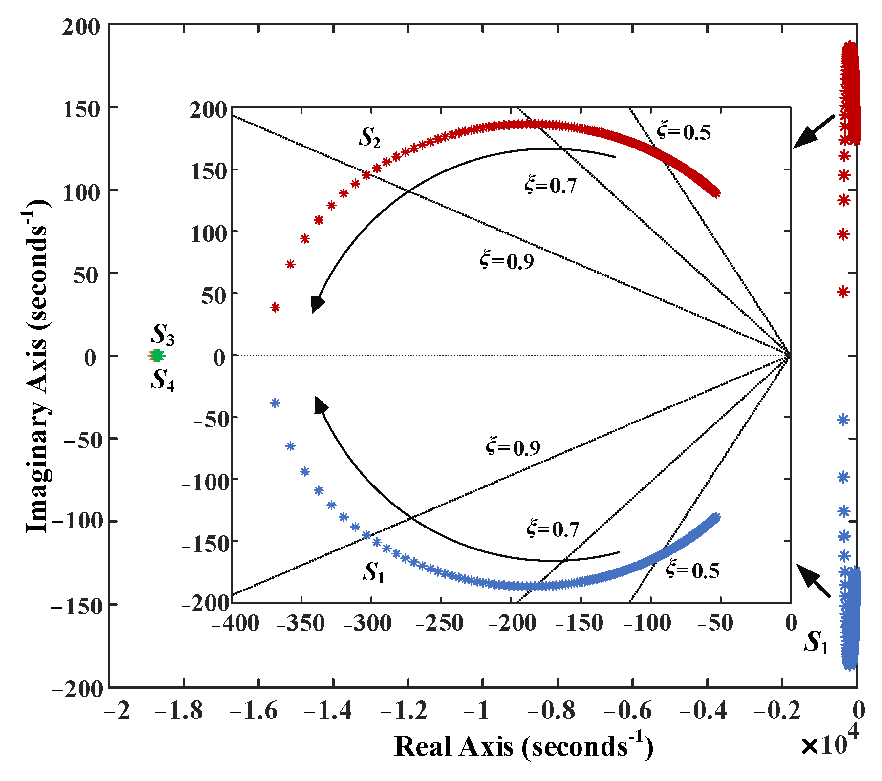
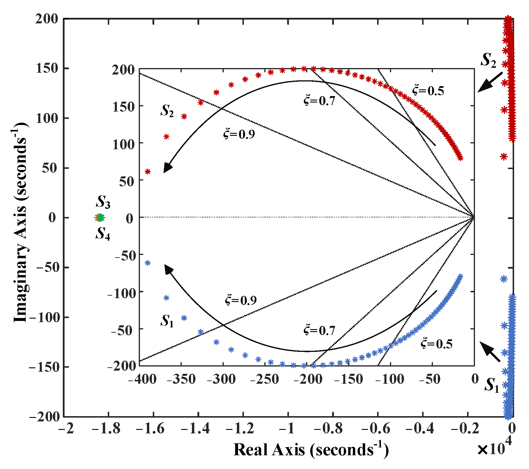
Figure 4 is the characteristic root locus diagram of the main control parameter $M_3$ changing from 0.001 to 0.004 while keeping main control parameters $M_4$, $W_3$, and $W_4$ unchanged. There are four characteristic roots in Equation (31) of the DFIG-IFLVSG grid-connected system, among which $S_3$ and $S_4$ are real roots that are almost constant, and their influence on the frequency stability of the system can be negligible. The characteristic roots in yellow and green are $S_3$ and $S_4$, respectively.

$S_1$ and $S_2$ are the conjugate complex roots, respectively, which are the dominant characteristic roots. The direction indicated by the arrow is the variation trend of the dominant characteristic roots in Figure 4. According to the results of the previous analyses, the gradual increase of $M_3$ gradually decreases $\left|\mathrm{d}\Delta \omega /\mathrm{d}t\right|$, thus decreases $\Delta {\omega }_{\mathrm{AMP}}$ and making the time for the system frequency to reach $\Delta {\omega }_{\mathrm{AMP}}$ longer. According to Figure 4, as $M_3$ gradually increases, $S_3$ and $S_4$ move away from the imaginary axis. In this case, the system damping ratio ξ also increases gradually, increasing the system stability. In addition, the active power overshoot and the system adjustment time are also reduced.

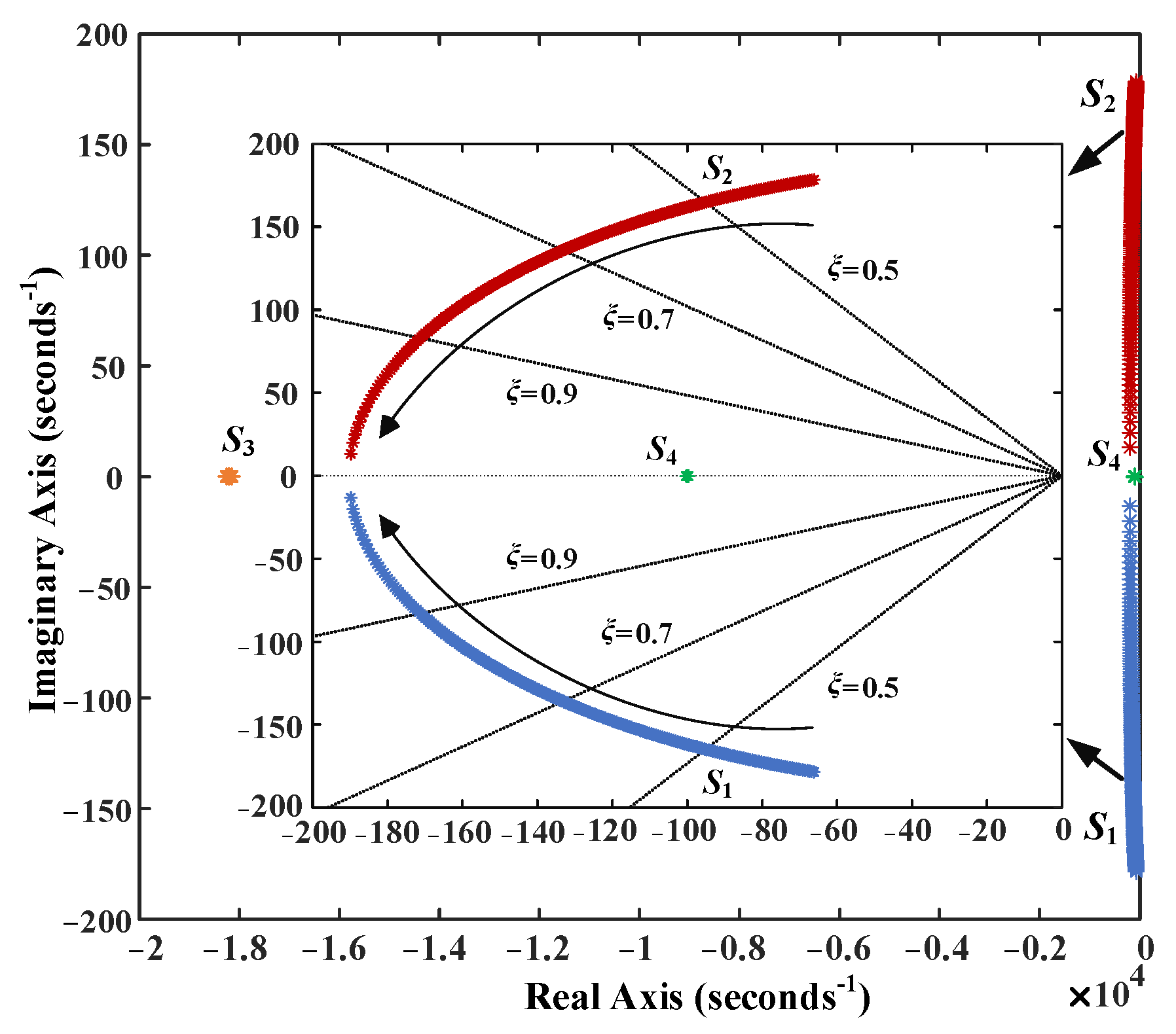
4.4.2. The Effect of the Control Parameter $M_4$ on the Frequency Stability of the System

Figure 5 is the characteristic root locus diagram of main control parameter $M_4$ changing from 1.05 to 1.35 while keeping the main control parameters $M_3$, $W_3$ and $W_4$ unchanged. At first, when $M_4$ is small, $K_{\mathrm{IFLd}}$ is also small. At this point, $\left|\mathrm{d}\Delta \omega /\mathrm{d}t\right|$ cannot be suppressed significantly, resulting in a large $\Delta {\omega }_{\mathrm{AMP}}$. In addition, the system frequency reaches $\Delta {\omega }_{\mathrm{AMP}}$ too prematurely. As M₄ increases, $\left|\mathrm{d}\Delta \omega /\mathrm{d}t\right|$ decreases significantly, thus decreasing $\Delta {\omega }_{\mathrm{AMP}}$. According to Figure 5, the gradual increase of ξ at this time leads to a decrease of both the active power overshoot and the system adjustment time. In addition, $S_3$ and $S_4$ also gradually move away from the imaginary axis with the increase of $M_4$, thus gradually increasing the system stability.

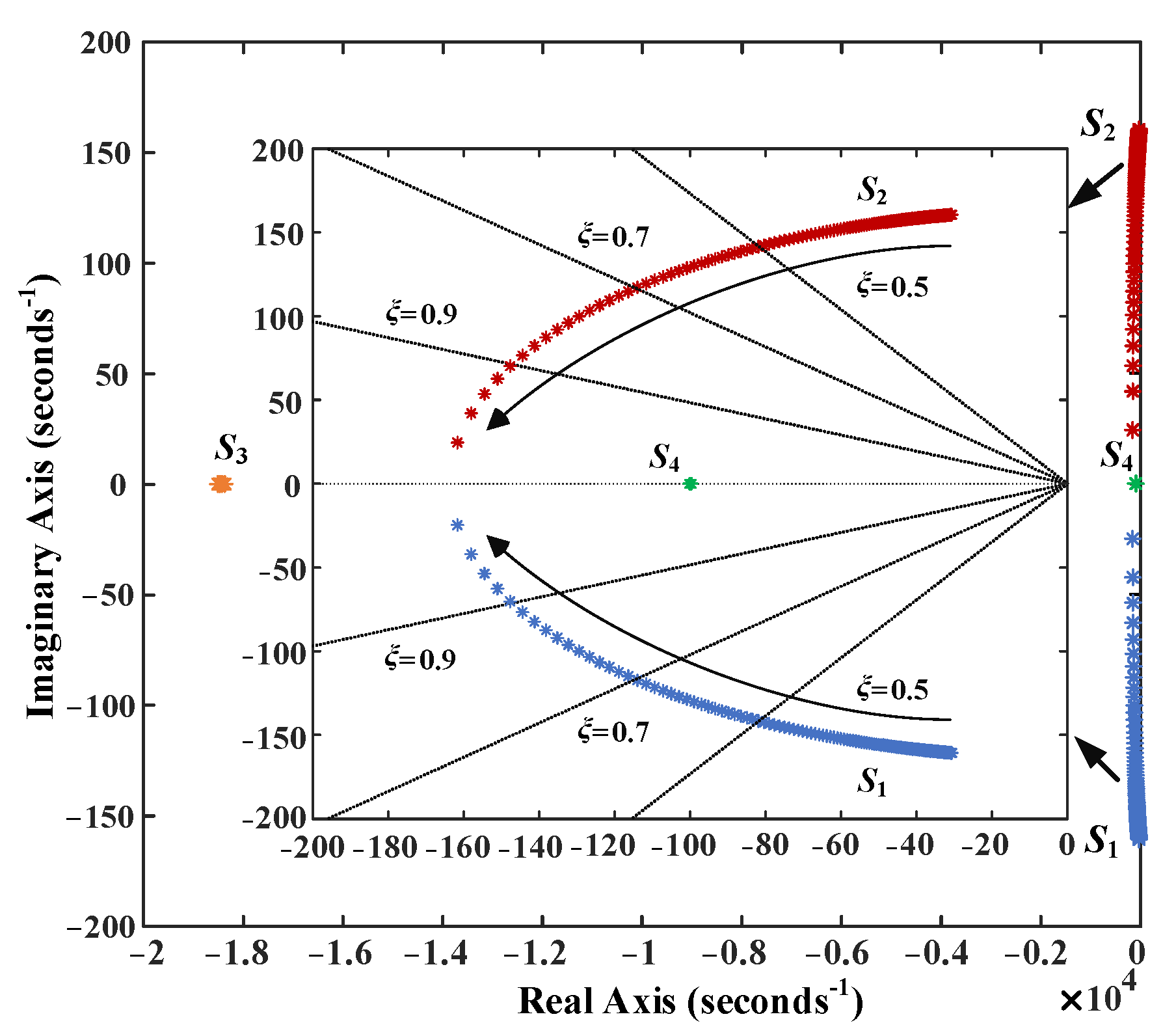
4.4.3. The Effect of the Control Parameter $W_3$ on the Frequency Stability of the System

Figure 6 is the characteristic root locus diagram of the main control parameter W₃ changing from 2 to 5 while keeping the main control parameters $M_3$, $M_4$ and $W_4$ unchanged. According to Figure 6, as $W_3$ increases, $K_{\mathrm{IFLp}}$ also increases gradually, and $S_1$ and $S_2$ gradually move away from the imaginary axis, leading to a gradual increase in system stability. Moreover, as $W_3$ increases, ξ gradually increases, leading to a gradual decrease in the active power overshoot and a corresponding decrease in the adjustment time.

4.4.4. The Effect of the Control Parameter $W_4$ on the Frequency Stability of the System

Figure 7 is the characteristic root locus diagram of the main control parameter $W_4$ changing from 1 to 3 while keeping the main control parameters $M_3$, $M_4$ and $W_3$ unchanged. According to Figure 7, as $W_4$ increases, $K_{\mathrm{IFLp}}$ increases, and $S_1$ and $S_2$ gradually move away from the imaginary axis, leading to a gradual increase in the system stability. Moreover, as $W_4$ increases, ξ gradually increases. However, with the increase of $W_3$ and $W_4$, $S_1$ and $S_2$ will eventually be subjected to a transition to the real axis, at which time the system will exhibit an over-damped state, leading to a slow system response [26].

5. Experimental Results

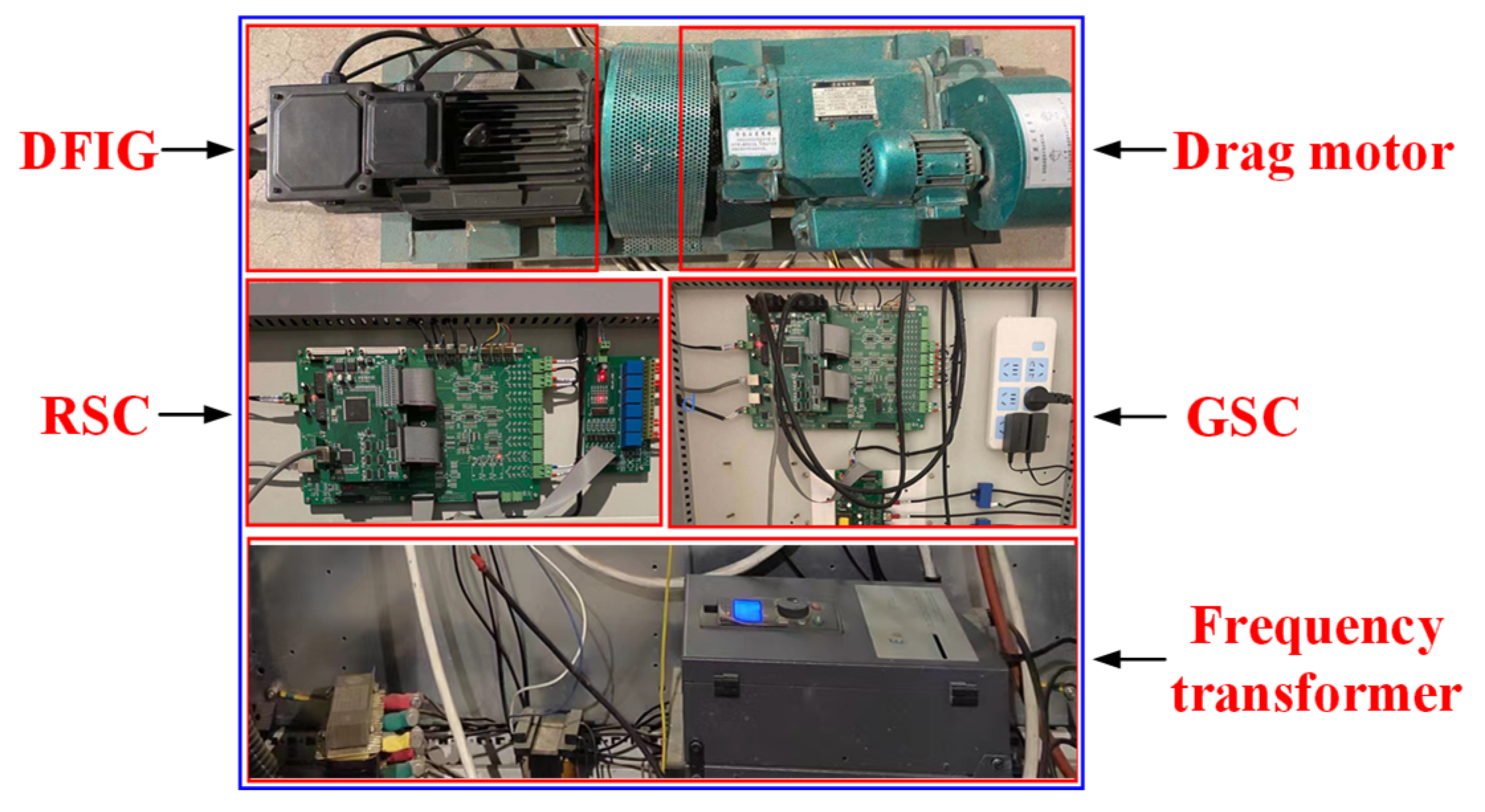
To further verify the superiority of the IFLVSG control strategy proposed in this study and the effectiveness of its control parameter selection law, a DFIG grid-connected hardware experimental platform was established. As shown in Figure 8, the platform consists of a Hall sensor, six sets of EPWM modules, an intelligent power module (IPM), an optoelectronic isolator, a drag motor, a frequency transformer, a Tamagawa 48-2500P8-L6-5V optical encoder, a DFIG, and converters on the stator side and the rotor side. All the above equipments are from Nanjing YanXu Electric Technology Co., Ltd. in China. By changing the rotation speed ${\omega }_r$ of the frequency transformer to simulate the change of wind speed, the active power command value $P_0$ is changed. The VSG and IFLVSG control strategies are embedded in the TMS320F28335 DSP with a switching frequency and a sampling frequency both of 10 kHz. Other hardware experimental platform parameters are listed in

Table A1. Parameters of the DFIG-IFLVSG wind power grid-connected system.

Parameter	Value	Parameter	Value
$R_{\sum }$	0.01325 Ω	$L_{\sum }$	0.037367 H
Rv	0.01 Ω	Lv	0.0373597 H
ω0	314 rad·s−1	P0	2.9 kW
J0	0.078 kg·m2	Dp0	20.26 N·m·s/rad
E0	380 V	Lm	0.0381 H
Rs	0.1726 Ω	Rr	0.1835 Ω
Ls	0.046476 H	Lr	0.048356 H
Pj	20 w	Td	0.4 rad·s−1
Tj	6.7 rad·s−2	Ta	0.01 s
Kpd	3	Kid	50
Kpq	3	Kiq	50
KpQ	0.001	KiQ	0.008

. To visually compare the experimental results, the different power and frequency data are exported and plotted in the same coordinate system by Matlab software, and the version of Matlab software used is 2021a, which was created by MathWorks company in the United States. The ${\omega }_r$ is set to increase abruptly at 20 s, at which time the changes in DFIG output power and system frequency are observed.

5.1. Superiority Verification of the IFLVSG Control Strategy

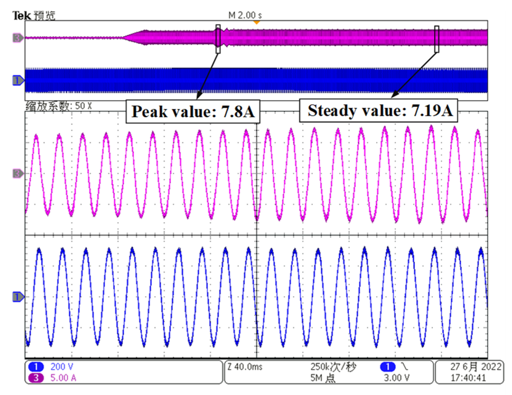
Figure 9 shows the waveforms of stator voltage and current. In Figure 9, ’缩放系数’ is zoom factor, ’次/秒’ is time per second. ’点’ is the point. As shown in Figure 9, DFIG achieves grid connection at approximately 10.5 s and reaches stability at approximately 13.3 s. The stator current and voltage in the steady state are 6.23 A and 311 V, respectively. As $P_0$ changes at 20 s, the stator current is adjusted from 6.23 A to 7.19 A. The stator current reaches a peak (7.8 A) during the change. By amplifying the stator current and voltage waveforms during 20.4 s–20.8 s, the stator current and voltage can be clearly observed.

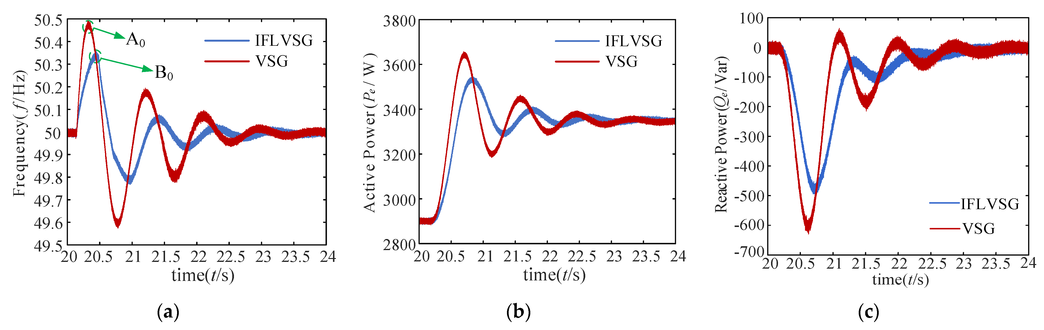
The comparison results of active power and its frequency of DFIG output based on VSG control strategy and IFLVSG control strategy are shown in Figure 10. ${\mathrm{A}}_0$ and ${\mathrm{B}}_0$ are the maximum frequency deviation points corresponding to VSG and IFLVSG, respectively. According to Figure 10, compared to the VSG control strategy, the active power output of DFIG based on IFLVSG control strategy has smaller overshoot σ% and less adjustment time $t_s$ when $\mathrm{d}\Delta \omega /\mathrm{d}t$, Δω, and $\Delta P_e$ all exceed the set thresholds. According to the analysis results in Section 3.2, $\mathrm{d}\Delta \omega /\mathrm{d}t$ is in the same direction as Δω when Δω does not reach the first peak, at which time $K_{\mathrm{IFLd}}$ in the IFLVSG control strategy can constrain $\mathrm{d}\Delta \omega /\mathrm{d}t$. Therefore, the frequency maximum point ${\mathrm{B}}_0$ of the IFLVSG control strategy is lower than that of the VSG control strategy ${\mathrm{A}}_0$. Similarly, according to Section 3.2 and the root locus analysis of $W_3$ and $W_4$, $K_{\mathrm{IFLp}}$ in the IFLVSG control strategy can reduce Δω and enhance the system stability. The σ% for the two control strategies are 8.806% and 5.075%, and $t_s$ are 1.124 s and 1.821 s, respectively. According to Figure 10c, it can be seen that compared with VSG, the overshoot and oscillation of the reactive power output of the DFIG output based on the IFLVSG control strategy are also significantly reduced. According to the expression of Equation (26), since the DFIG operates at a unit power factor, that is, $Q_0=0$, the reactive power $Q_e$ of the DFIG output based on the two control strategies finally reaches a steady-state value of about zero. Figure 10 verifies the correctness of the theoretical analyses and the superiority of the IFLVSG control strategy.

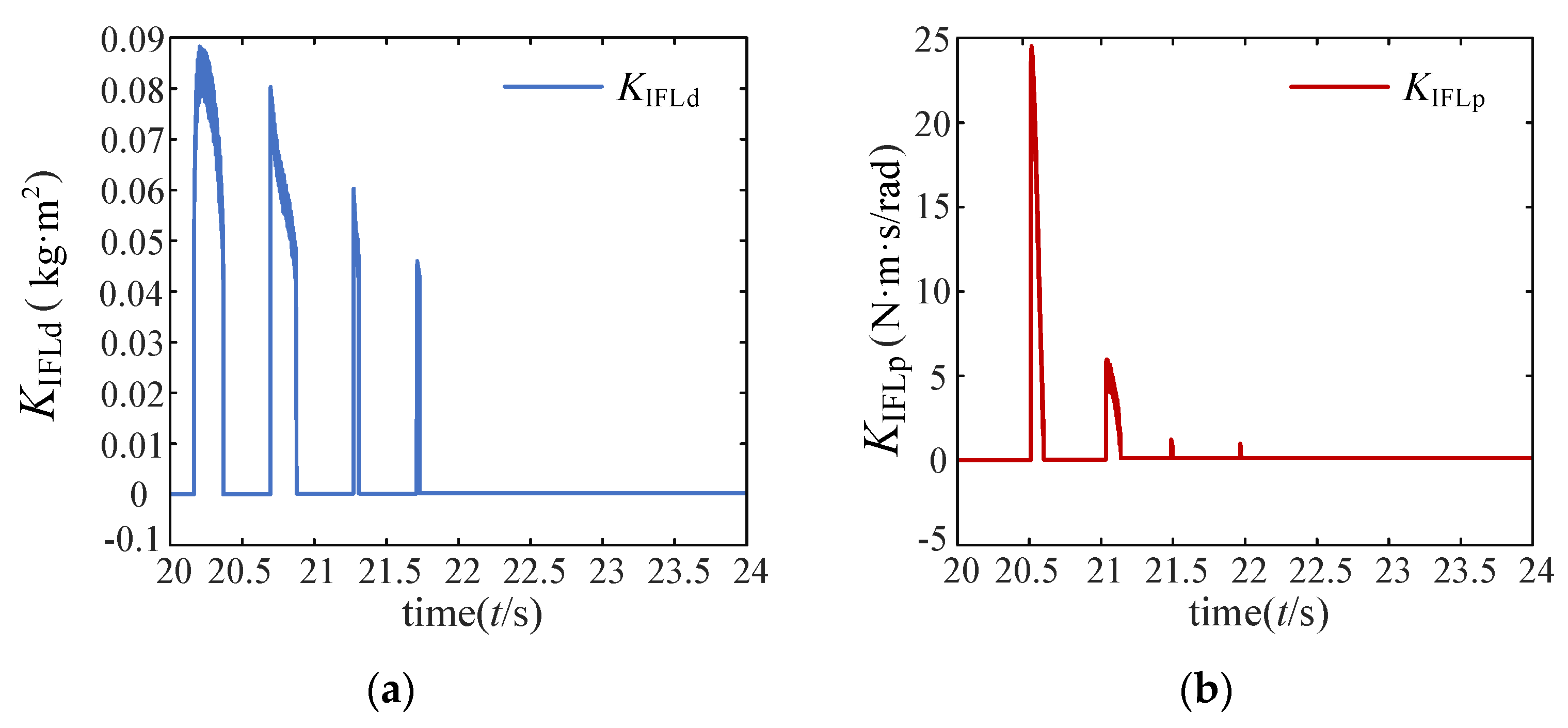
Figure 11 shows the results of $K_{\mathrm{IFLd}}$ and $K_{\mathrm{IFLp}}$. In Figure 11, $K_{\mathrm{IFLd}}$ and $K_{\mathrm{IFLp}}$ are changed according to Equations (20) and (21) and the selection rules in Table 1, and the change process is smooth and stable. According to the analysis in Section 3.2.3, $K_{\mathrm{IFLd}}$ and $K_{\mathrm{IFLp}}$ can be continuously adjusted according to the change of system frequency, so the change range of $K_{\mathrm{IFLd}}$ and $K_{\mathrm{IFLp}}$ is wide. According to the above analysis of the oscillation curve in Figure 2 and Equations (14) and (15), $K_{\mathrm{IFLd}}$ and $K_{\mathrm{IFLp}}$ are equivalent to increase $J_0$ and $D_{p0}$ within the defined interval, respectively, so as to improve the frequency stability of the system. Figure 11 verifies the correctness of the theoretical analyses.

5.2. Verification and Analysis on the Influence Laws of the Change of the Main Control Parameters on the System

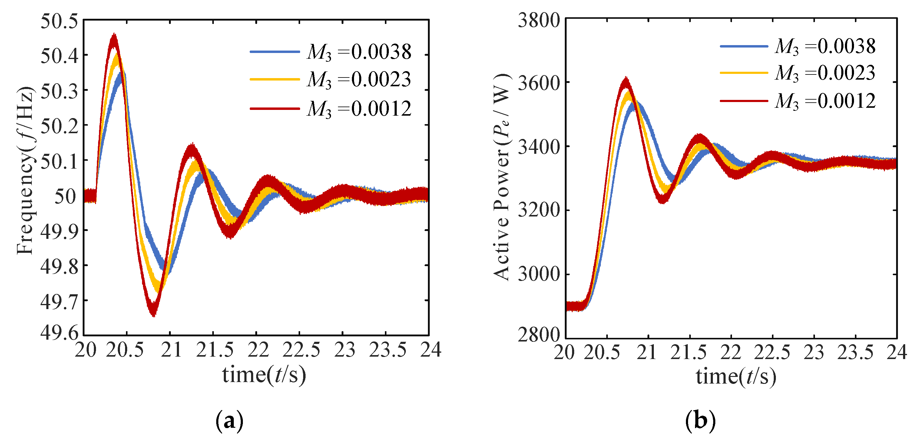
Figure 12a,b show the response plots of the DFIG-output active power and system frequency when the value of $M_3$ changes. In Figure 12, $M_3$ gradually increases, and the values are 0.0012, 0.0023, and 0.0038, respectively. As can be seen from Figure 12, with the increases of $M_3$, the overshoot σ% and the adjustment time $t_s$ of the DFIG-output active power are gradually decreased, leading to the enhancement of the stability of the wind power grid-connected system. In addition, the maximum point of frequency decreases significantly with the increase of $M_3$. When $M_3$ = 0.0012, the maximum point of frequency is close to the maximum allowable value of frequency (50.5 Hz), which poses a serious threat to the frequency stability and is not conducive to the dynamic stability of the system.

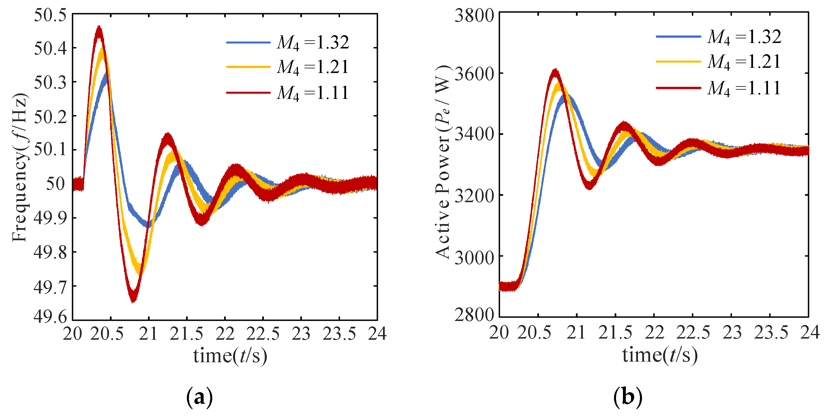
Figure 13a,b show the response plots of the DFIG-output active power and system frequency when the value of $M_4$ changes. In Figure 13, $M_4$ gradually increases, and the values are 1.11, 1.21, and 1.32, respectively. According to the analysis results in Section 4.4, with the increase of $M_4$, the system damping ratio ξ gradually increases. As can be seen from Figure 13, with the increases of M₄, both σ% and $t_s$ decrease gradually. In addition, the increase of $M_4$ suppresses the increase of $\mathrm{d}\Delta \omega /\mathrm{d}t$, thus significantly reducing the highest point of frequency. When $M_4$ = 1.11, the highest point of frequency is close to the maximum allowable value of frequency (50.5 Hz), which impairs the frequency stability and is not conducive to the dynamic stability of the system.

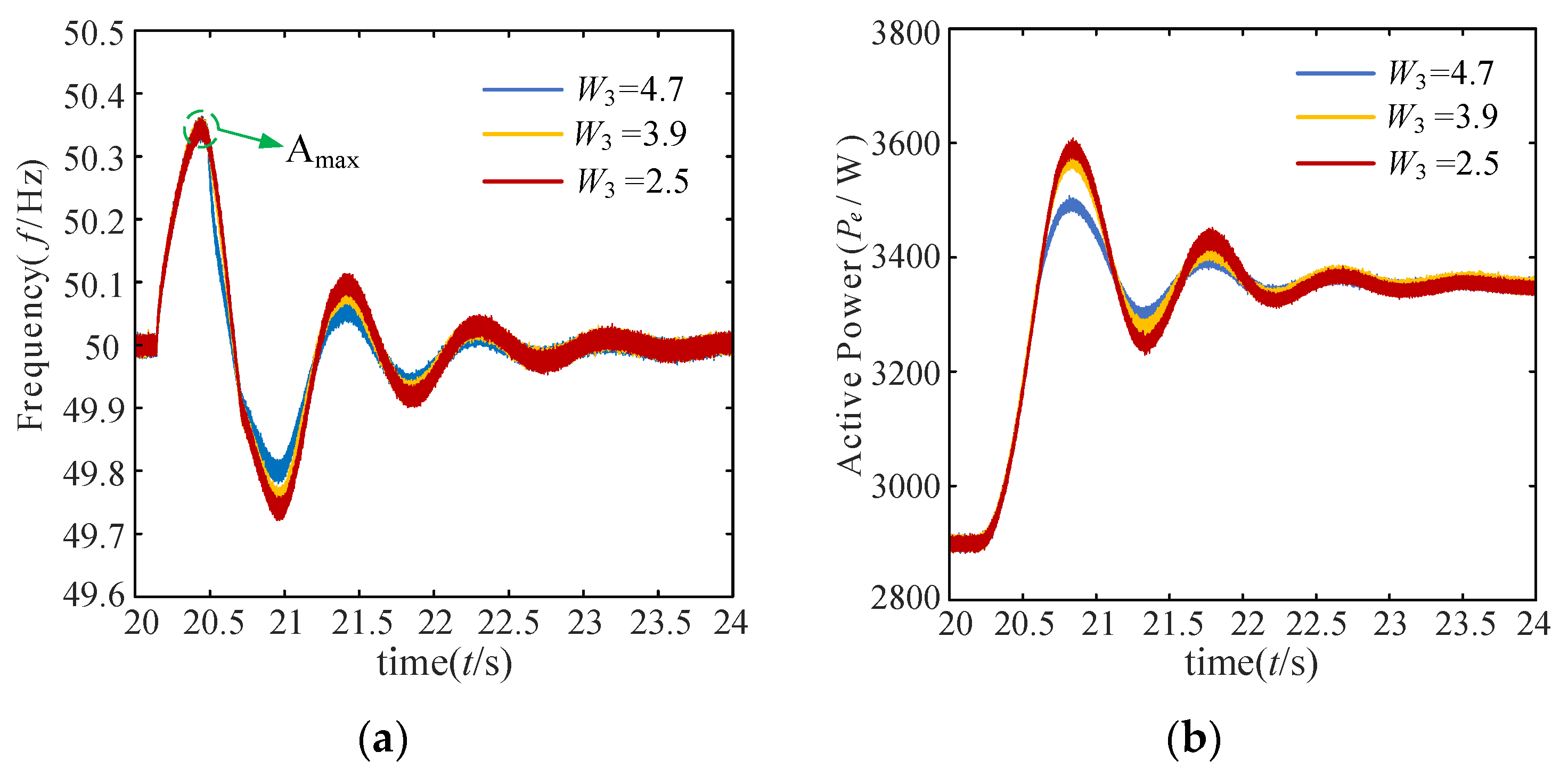
Figure 14a,b show the response plots of the DFIG-output active power and the system frequency when the value of $W_3$ changes. In Figure 14, $W_3$ gradually increases, and the values are 2.5, 3.9, and 4.7, respectively, and A_max is the maximum frequency deviation point corresponding to different $W_3$. As can be seen from Figure 14, with the increases of $W_3$, both σ% and t_s gradually decrease, and the oscillations of active power and frequency also gradually decrease. However, when P₀ is changed, according to Figure 2 and its analysis results, Δω and $\mathrm{d}\Delta \omega /\mathrm{d}t$ are in the same direction when Δω has not reached the highest point. In this case, only $K_{\mathrm{IFLd}}$ is involved in the tuning of the frequency, whereas $K_{\mathrm{IFLp}}$ is not. Therefore, despite the change in the value of $W_3$ or $W_4$, neither A_max nor B_max, the highest points of frequency in Figure 14 and Figure 15, change. According to the analysis results in Section 3.2, $K_{\mathrm{IFLp}}$ is equivalent to an equivalent increase in damping coefficient. Therefore, the changes in $W_3$ and $W_4$ have little effect on the inertia characteristics of the DFIG-IFLVSG. Therefore, change in $W_3$ has a large effect almost only on the active power output of the DFIG and the change amplitude of its frequency.

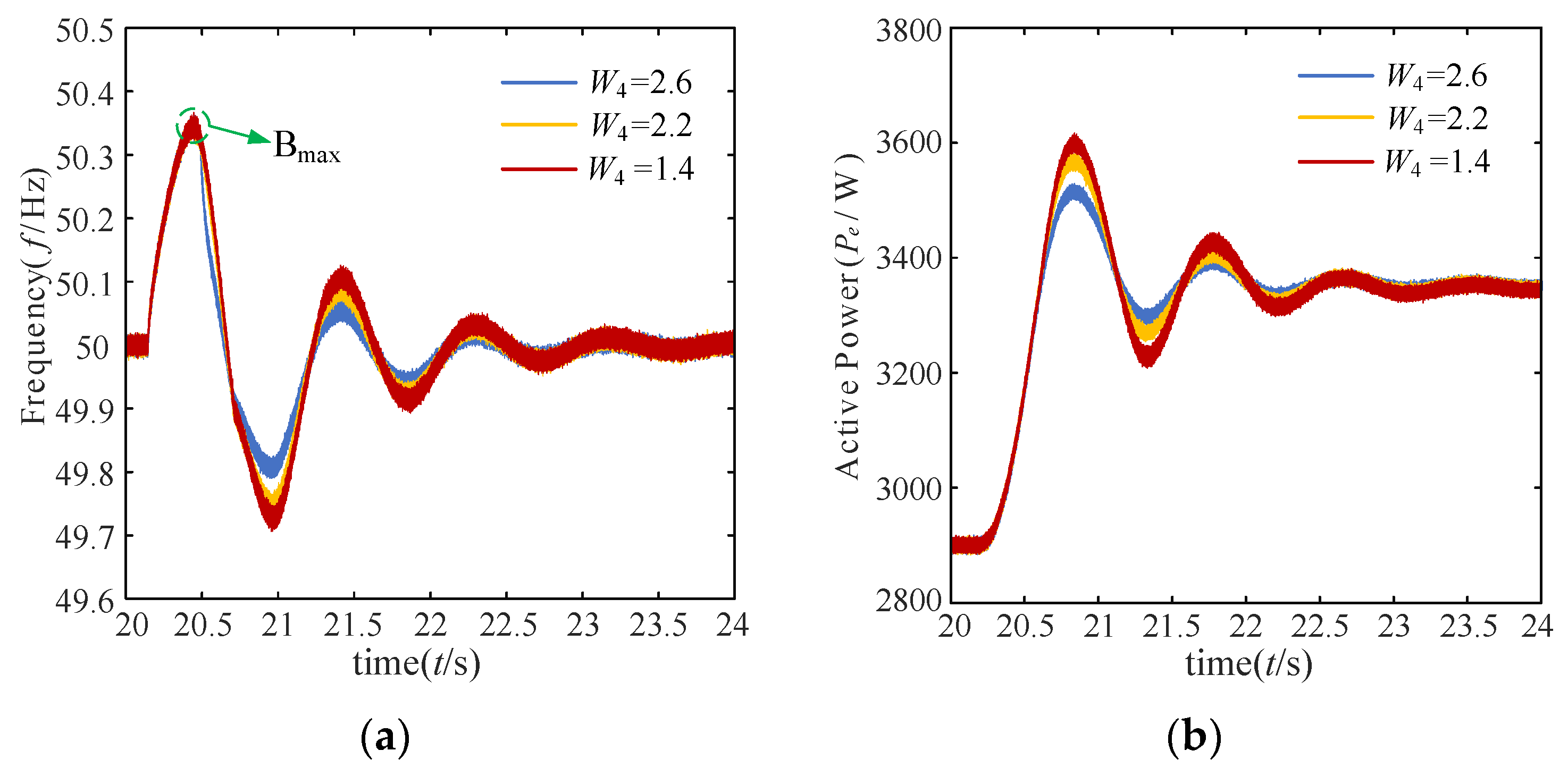
Figure 15a,b show the response plots of the DFIG-output active power and the system frequency when the value of $W_4$ changes. In Figure 15, $W_4$ gradually increases, and the values are 1.4, 2.2, and 2.6, respectively, and B_max is the maximum frequency deviation point corresponding to different $W_4$. As can be seen from Figure 15, with the increases of $W_4$, both σ% and $t_s$ gradually decrease, and the oscillations of active power and frequency also gradually decrease. According to the analysis results in Section 4.4, the gradual increase in $W_3$ and $W_4$ gradually increases the system damping ratio ξ, thus enhancing the system stability.

However, when the value of $W_3$ or $W_4$ is too large, the consequent large $K_{\mathrm{IFLp}}$ results in large damping coefficient of the DFIG-IFLVSG, which influences the active power output characteristics of the DFIG-IFLVSG.

Table 3. t_s and σ% of the different values.

Parameter	ts (s)	σ%
M3 = 0.0012	1.752 s	7.462%
M3 = 0.0023	1.333 s	6.268%
M3 = 0.0038	1.119 s	4.776%
M4 = 1.11	1.763 s	7.611%
M4 = 1.21	1.211 s	6.119%
M4 = 1.32	1.103 s	4.716%
W3 = 2.5	1.728 s	7.223%
W3 = 3.9	1.408 s	6.567%
W3 = 4.7	1.046 s	4.239%
W4 = 1.4	1.812 s	7.821%
W4 = 2.2	1.228 s	6.238%
W4 = 2.6	1.121 s	4.925%

shows the different values of $M_3$, $M_4$, $W_3$ and $W_4$, the corresponding $t_s$ and σ%.

6. Conclusions

On the basis of not changing the structure and parameters of the VSG control strategy, this paper proposed an exponential IFLVSG control strategy to improve the frequency stability of wind power grid-connected systems, and formed a complete parameter selection scheme by constructing a state space equation, performing sensitivity calculation, and conducting root locus analysis, thus providing a theoretical basis for the selection of IFL control parameters. The conclusions are as follows:

• The advantage of the exponential IFLVSG control strategy is clarified by the sensitivity calculation method. To better improve the stability of the wind power grid-connected system, three typical IFLVSG control strategies are studied. According to the variable range of $K_{\mathrm{IFLd}}$ and $K_{\mathrm{IFLp}}$, and the sensitivity of the system frequency stability to the change of control parameters in the IFL, the advantages of the exponential IFLVSG control strategy are highlighted;
• Rely on the sensitivity calculation method to improve the analysis efficiency. According to the sensitivity calculation method, all parameters in the state space equation, including the IFLVSG control strategy, are calculated. While it is concluded that the main control parameters affecting the frequency stability of the system are $M_3$, $M_4$, $W_3$, and $W_4$, it is also possible to avoid further in-depth analysis of other parameters, thus improving the analysis efficiency;
• Reveal the influence law of control parameters on the stability of the system frequency system. The root locus analysis method reveals the influence law of the main control parameters $M_3$, $M_4$, $W_3$, and $W_4$ on the stability of the system frequency, that is, with the increase of $M_3$ and $M_4$, ξ gradually increases, t_s and σ% are reduced, and can reduce the maximum deviation of the system frequency while suppressing the change rate of the system frequency. With the increase of $W_3$ and $W_4$, ξ also gradually increases, t_s and σ% decrease, and the change of $W_3$ and $W_4$ has no effect on the maximum deviation of the system frequency.

References

- Miyazaki, S.; Mizutani, Y. Method of Evaluating Probability of Pressboard Failure in Power Transformer with DiscType Winding due to Electromagnetic Force by External Short Circuit. IEEJ Trans. Electr. Electron. Eng. 2021, 16, 973–981. [Google Scholar] [CrossRef]
- Nian, H.; Jiao, Y. Improved Virtual Synchronous Generator Control of DFIG to Ride-Through Symmetrical Voltage Fault. IEEE Trans. Energy Convers. 2019, 35, 672–683. [Google Scholar] [CrossRef]
- Tian, X.; Wang, W.; Chi, Y.; Li, Y.; Liu, C. Virtual inertia optimisation control of DFIG and assessment of equivalent inertia time constant of power grid. IET Renew. Power Gener. 2018, 12, 1733–1740. [Google Scholar] [CrossRef]
- Wang, S.; Hu, J.; Yuan, X.; Sun, L. On Inertial Dynamics of Virtual-Synchronous-Controlled DFIG-Based Wind Turbines. IEEE Trans. Energy Convers. 2015, 30, 1691–1702. [Google Scholar] [CrossRef]
- Han, J.; Liu, Z.; Liang, N. Nonlinear Adaptive Robust Control Strategy of Doubly Fed Induction Generator Based on Virtual Synchronous Generator. IEEE Access 2020, 8, 159887–159896. [Google Scholar] [CrossRef]
- Fu, Y.; Wang, Y.; Zhang, X. Integrated wind turbine controller with virtual inertia and primary frequency responses for grid dynamic frequency support. IET Renew. Power Gener. 2017, 11, 1129–1137. [Google Scholar] [CrossRef]
- Ma, Y.; Cao, W.; Yang, L.; Wang, F.; Tolbert, L.M. Virtual Synchronous Generator Control of Full Converter Wind Turbines with Short Term Energy Storage. IEEE Trans. Ind. Electron. 2017, 64, 8821–8831. [Google Scholar] [CrossRef]
- Liu, J.; Miura, Y.; Ise, T. Comparison of Dynamic Characteristics between Virtual Synchronous Generator and Droop Control in Inverter-Based Distributed Generators. IEEE Trans. Power Electron. 2016, 31, 3600–3611. [Google Scholar] [CrossRef]
- Torres, L.; Miguel, A.; Lopes, L.A.; Moran, T.L.A.; Espinoza, C.J.R. Self-Tuning Virtual Synchronous Machine: A Control Strategy for Energy Storage Systems to Support Dynamic Frequency Control. IEEE Trans. Energy Convers. 2014, 29, 833–840. [Google Scholar] [CrossRef]
- Alipoor, J.; Miura, Y.; Ise, T. Power System Stabilization Using Virtual Synchronous Generator with Alternating Moment of Inertia. IEEE J. Emerg. Sel. Top. Power Electron. 2014, 3, 451–458. [Google Scholar] [CrossRef]
- Dong, J.; Wang, L. Study on an Adaptive Virtual Synchronous Generator Control Strategy for Distributed Generators. Electr. Drive 2019, 49, 78–81. [Google Scholar]
- Ren, M.; Li, T.; Shi, K.; Xu, P.; Sun, Y. Coordinated Control Strategy of Virtual Synchronous Generator Based on Adaptive Moment of Inertia and Virtual Impedance. IEEE J. Emerg. Sel. Top. Circ. Syst. 2021, 11, 99–110. [Google Scholar] [CrossRef]
- Wang, Y.; Hei, Y.; Fu, Y.; Shi, K. Adaptive Virtual Inertia Control of DC Distribution Network Based on Variable Droop Coefficient. Autom. Electr. Power Syst. 2017, 41, 116–124. [Google Scholar]
- Karimi, A.; Khayat, Y.; Naderi, M.; Dragičević, T.; Mirzaei, R.; Blaabjerg, F.; Bevrani, H. Inertia Response Improvement in AC Microgrids: A Fuzzy-Based Virtual Synchronous Generator Control. IEEE Trans. Power Electron. 2020, 35, 4321–4331. [Google Scholar] [CrossRef]
- Li, M.; Huang, W.; Tai, N.; Yang, L.; Duan, D.; Ma, Z. A Dual-Adaptivity Inertia Control Strategy for Virtual Synchronous Generator. IEEE Trans. Power Syst. 2019, 35, 594–604. [Google Scholar] [CrossRef]
- Xie, Z.; Meng, H.; Zhang, X.; Jin, X.W. Virtual Synchronous Control Strategy of DFIG-based Wind Turbines Based on Stator Virtual Impedance. Autom. Electr. Power Syst. 2018, 42, 157–163. [Google Scholar]
- Li, T.; Wen, B.; Wang, H. A Self-Adaptive Damping Control Strategy of Virtual Synchronous Generator to Improve Frequency Stability. Processes 2020, 8, 291. [Google Scholar] [CrossRef]
- Yao, F.; Zhao, J.; Li, X.; Mao, L.; Qu, K. RBF Neural Network Based Virtual Synchronous Generator Control with Improved Frequency Stability. IEEE Trans. Ind. Inform. 2020, 17, 4014–4024. [Google Scholar] [CrossRef]
- Wang, F.; Zhang, L.; Feng, X.; Guo, H. An Adaptive Control Strategy for Virtual Synchronous Generator. IEEE Trans. Ind. Appl. 2018, 54, 5124–5133. [Google Scholar] [CrossRef]
- Li, D.; Zhu, Q.; Lin, S.; Bian, X.Y. A Self-Adaptive Inertia and Damping Combination Control of VSG to Support Frequency Stability. IEEE Trans. Energy Convers. 2016, 32, 397–398. [Google Scholar] [CrossRef]
- He, Y.; Hu, J. Several Hot-spot Issues Associated with the Grid-connected Operations of Wind-turbine Driven Doubly Fed Induction Generators. Proc. Chin. Soc. Electr. Eng. 2012, 32, 1–15. [Google Scholar]
- Tan, Y.; Meegahapola, L.; Muttaqi, K.M. A Suboptimal Power-Point-Tracking-Based Primary Frequency Response Strategy for DFIGs in Hybrid Remote Area Power Supply Systems. IEEE Trans. Energy Convers. 2015, 31, 93–105. [Google Scholar] [CrossRef]
- Cheng, X.; Liu, H.; Tian, Y.; Tian, Y. Review of Transient Power Angle Stability of Doubly-fed Induction Generator with Virtual Synchronous Generator Technology Integration System. Power Syst. Technol. 2021, 45, 518–525. [Google Scholar]
- Meng, Z.; Hou, Y.; Fang, Y.; Fang, Y. Analysis on Large Disturbance Power-angle Stability of Strong-damping Voltage-source Virtual Synchronous Generators. Autom. Electr. Power Syst. 2018, 42, 44–50. [Google Scholar]
- Huang, L.; Zhang, L.; Xin, H.; Hu, J.; Gan, D. Mechanism Analysis of Virtual Power Angle Stability in Droop-Controlled Inverters. Autom. Electr. Power Syst. 2016, 40, 117–124. [Google Scholar]
- Luo, C.H.; Zhang, F.Z. Application of MATLAB Language in Teaching of Automatic Control Principles. J. Electr. Electron. Eng. Educ. 2003, 3, 53–56. [Google Scholar]
Publisher’s Note: MDPI stays neutral with regard to jurisdictional claims in published maps and institutional affiliations. |
© 2022 by the authors. Licensee MDPI, Basel, Switzerland. This article is an open access article distributed under the terms and conditions of the Creative Commons Attribution (CC BY) license (https://creativecommons.org/licenses/by/4.0/).