The Adaptive Streaming SAR Back-Projection Algorithm Based on Half-Precision in GPU

Abstract

The back-projection (BP) algorithm is completely accurate in the imaging principle, but the computational complexity is extremely high. The single-precision arithmetic used in the traditional graphics processing unit (GPU) acceleration scheme has low throughput and its usage of the video memory is large. An adaptive asynchronous streaming scheme for the BP algorithm based on half-precision is proposed in this study, and then it is extended to the fast back-projection (FBP) algorithm. In this scheme, the adaptive loss factors selection strategy ensures the dynamic range of data, the asynchronous streaming structure ensures the efficiency of large scene imaging, and the mixed-precision data processing ensures the imaging quality. The schemes proposed in this paper are compared with BP, FBP, and fast factorized back-projection (FFBP) algorithms of single-precision in GPU. The experimental results show that the two half-precision acceleration schemes in this paper reduce the video memory usage to 74% and 59% of the single-precision schemes with guaranteed image quality. The efficiency improvements of the proposed schemes are almost one and 0.5 times greater than that of the corresponding single-precision scheme, and the advantage can be more obvious when dealing with large computations.

1. Introduction

The back-projection (BP) algorithm originates from computed tomography (CT), which is a point-by-point time-domain imaging algorithm without any approximation [1]. However, due to its computational complexity of O (N^3), it is difficult to achieve the requirement of real-time imaging. Digital signal processor (DSP) and field programmable gate array (FPGA) technologies in synthetic aperture radar (SAR) real-time imaging can achieve considerable acceleration ratios, but the programming to the hardware system is complex and the equipment is expensive [2,3].

In order to reduce the computational volume, a fast back-projection (FBP) algorithm [4,5] and a fast factorized back-projection (FFBP) algorithm [6] are proposed to improve the original BP algorithm. The difference between the FBP algorithm and the original BP algorithm is that it divides the total synthetic aperture into several small sub-apertures. The imaging process for each sub-aperture polar coordinate system is the same as that of the original BP algorithm, and the images formed by all sub-apertures are fused into one full-aperture scene image. The first step of the FFBP algorithm is also the sub-aperture division of the synthetic aperture to obtain lower resolution sub-aperture images. However, for the obtained sub-aperture images, FFBP does not directly fuse them into a full-aperture scene image. A certain fusion base is selected, and then a group of sub-apertures is used to fuse the images into a higher resolution sub-aperture scene image. This process is repeated until the number of sub-apertures is less than or equal to the merge-base. Finally, several sub-images are interpolated and fused into the full-aperture image with the same operation as FBP.

In June 2007, NVIDIA introduced the compute unified device architecture (CUDA) with a C-like programming language, making high-performance parallel computing under the graphics processing unit (GPU) gradually come into the public view [7]. In current studies on GPU-accelerated SAR imaging, significant accelerating effects have been achieved with different acceleration and optimization methods [8,9,10,11,12,13,14,15,16,17,18,19,20,21]. Fasih et al. proposed a parallel acceleration scheme in the BP algorithm, which divided data into partitions according to range and aperture, and implemented interpolation based on texture memory. In this acceleration scheme, the grid, block, and thread corresponded to image, sub-image, and pixel, respectively [13]. However, the acceleration effect of this scheme was unfavorable, and the problem of large data volume in real-time imaging was not considered. Meng et al. from the Institute of Electronics, Chinese Academy of Sciences, elaborated an optimization method for GPU parallel programs to solve the problem of insufficient GPU video memory in data transfer and data processing, improving the real-time processing speed of the device under large data volume. Their study was focused on frequency domain SAR imaging, and the real-time performance of imaging can still be improved [12]. Liu used remote direct memory access (RDMA) technology to realize multi- GPU collaborative computing of the BP algorithm [20]. The FBP and FFBP algorithms are technically identical to the BP algorithm and also have a high degree of parallelism, which allows a significant increase in efficiency using GPU parallelism [18,22,23,24].

Unlike the improvements in the above GPU-based parallel scheme, the precision of the data processing can also have a significant impact on the imaging efficiency. Portillo et al. evaluated the impact of floating-point precision on radar image quality and power and energy consumption. It was found that using a mixture of the single-precision floating point (FP32) and double-precision floating point (FP64) imaging can achieve relatively higher image quality with lower power consumption [8]. M. Wielage et al. compared the acceleration effect and power consumption of the FFBP algorithm with FP32 and half precision on GPU and FPGA platforms, respectively [18]. In addition, single-precision accelerated SAR algorithms were investigated in many studies, and many good results were achieved by reducing the precision [9,10,11,18].

In version 7.5 of CUDA, the half-precision floating point (FP16) was introduced [25]. The low-precision arithmetic enables less video memory usage, greater computational throughput, and shorter access times, but its low dynamic range of data and high representation errors pose challenges for the imaging quality [26]. Currently, FP16 arithmetic has been widely used in deep learning, and considerable acceleration ratios have been obtained by loss calibration, mixed-precision arithmetic, and other methods to guarantee model accuracy [27,28]. Currently, there are three main constraints to achieve FP16 arithmetic for real-time BP imaging, which are described as follows:

• The dynamic range of the data. Compared with FP64/ FP32 arithmetic, FP16 arithmetic displays a smaller range of data, so it is challenging to cope with the inevitable order-of-magnitude fluctuations in the processing of measured data.
• The low accuracy. The FP16 arithmetic has a higher data representation error, especially in trigonometric computing with high accuracy requirements. The error can directly lead to unacceptable imaging results.
• The asymmetric relationship between the measured data volume and the memory capacity. The existing GPUs have small memory, and the SAR imaging data volume is large; the GPU memory can hardly support the reading and processing of the SAR echo data, and the transmission time of the large volume of data between the device and the host is very long.

Regarding the above problems, an adaptive asynchronous streaming acceleration scheme is proposed, which improves real-time data processing while ensuring imaging quality. In this scheme, data is reduced to FP16 for storage, transmission, and calculation, and the data processing and memory copy are parallelized.

The rest of this paper is organized as follows. The BP algorithm, FBP algorithm, FFBP algorithm, and their parallel computing models are introduced in Section 2. Section 3 presents an adaptive asynchronous streaming BP algorithm acceleration scheme based on FP16 arithmetic, and extends it to the FBP algorithm, and the optimization strategy and error analysis are described in detail in this section. Section 4 includes the experimental results and corresponding analysis, and conclusions are described in Section 5.

2. Research Method

2.1. BP Algorithm and GPU Acceleration Model

The SAR BP algorithm mainly consists of two parts: range compression and back projection. The range compression equation can be expressed as:

$$s_M\left(\tau ,\eta \right)=s_r\left(\tau ,\eta \right)\otimes h\left(\tau \right)$$

(1)

where $\tau$ represents the range time; $\eta$ represents the azimuthal time; $s_r\left(\tau ,\eta \right)$ represents the echo signal.

The range compression function $h\left(\tau \right)$ can be obtained:

$$h\left(\tau \right)=\mathrm{rect}\left(\frac{\tau }{T_r}\right)\exp (-j\pi K_r{\tau }^2)$$

(2)

where $K_r$ is the linear modulation frequency; rect() represents the rectangular window function; $T_r$ is the pulse duration.

The back projection is divided into several steps: division of the grid, calculation of the two-way delay, linear interpolation, phase compensation, and coherent addition of the signal. The back projection equation can be expressed as follows:

$$f_{BP}\left(x_m,y_n\right)=\int s_M\left[{\tau }_{mn}\left(\eta \right),\eta \right]\exp (\frac{j4\pi R_{mn}}{\lambda })d\eta$$

(3)

where $\lambda$ represents the radar emission wavelength; ${\tau }_{\mathrm{mn}}\left(\eta \right)$ indicates the delay between the point and the radar; $R_{\mathrm{mn}}$ is the distance from the point $\left(x_m,y_n\right)$ to the radar $\left(0,y\left(\eta \right)\right)$:

$$R_{\mathrm{mn}}=\sqrt{{x_m}^2+{(y\left(\eta \right)-y_n)}^2}$$

(4)

In this model, the central processing unit (CPU) holds the overall architecture of the algorithm and transfers the data to the global memory of the GPU. Then, the kernel function is started on the GPU to read the global memory and complete the parallel data processing. Finally, the processed data is sent back to the CPU. However, because the transfer speed of the input/output (I/O) between the global memory and the CPU is slow, frequent data interactions can reduce efficiency, and the delay effect is more obvious in big data imaging [9].

Currently, the parallel strategy shown in Figure 1 is usually adopted in existing BP algorithm acceleration schemes [29]. Range compression is achieved by transferring the data to the frequency domain with the help of the CUDA batch fast Fourier transform (FFT) function cufftExecC2C(). The compressed data is converted back to the time domain by the batch inverse fast Fourier transform (IFFT) function. However, the GPU computing module is idle for a long time during data transfer. CUDA provides a copy function, cudaMemcpyAsync(), which enables the early return of control between the device and host [30]. By allocating the same instructions to different streams in a batch, the original instructions are subdivided, operations within each stream are implemented sequentially, and parallel implementation can be achieved between different streams. In addition, the thread synchronization can be completed by the cudaThreadSynchronize() instruction.

As mentioned above, the use of asynchronous parallel streaming technology in batches allows the computation of one stream to be performed simultaneously with the data copy of another stream, concealing the data copy time and reducing the video memory usage. In order to meet the processing requirements of large data volume, the GPU scheme in this paper changes the range compression and back projection of Figure 1 to an asynchronous streaming structure. The volume of data processed by each stream is very small and is passed back to the CPU when the processing is complete. Therefore, the data transfer time is concealed. The internal process of the back projection kernel in the BP algorithm remains unchanged, and each thread is responsible for calculating the total contribution of that data block to a particular pixel point. The flow of the range compression in asynchronous streams is schematically shown in Figure 2.

Thus, the data copy is completed first in each stream. Number 1, 2, and 3 in Figure 2 represent the range compression, adaptive loss factors selection, and data precision conversion implementation, respectively. Since the FP32 dynamic range can meet the processing requirements, steps 2 and 3 are only used in the proposed FP16 schemes, which are detailed in Section 3.

According to the description above, the data is bifurcated according to batch and stream, and the number of azimuth pulses $Nu$ of each data block can be evenly divided by the batch and stream number.

It is assumed that i and j represent the jth stream data block of batch i. Due to the limitation of synthetic aperture length $Ls$, the number of signals corresponding to each imaging point is limited in the strip mode. In the BP algorithm, the lower bound index $lo{w}_{i,j} and$ the upper bound index $uppe{r}_{i,j}$ of imaging region in video memory of each data block can be obtained by Equations (5) and (6), respectively. In the back projection of a specific data block, only the threads with thread IDs in the region need to be implemented:

$$lo{w}_{i,j}=\left\{\begin{array}{c}0\\ \left|\frac{y_{i,j_{min}}-\frac{Ls}{2}-W{y}_{min}}{dy}\right|\end{array}\right.\begin{array}{c}{y}_{i,j_{min}}-\frac{Ls}{2}-W{y}_{min}<0\\ \\ else\end{array}$$

(5)

$$uppe{r}_{i,j}=\left\{\begin{array}{c}Ny-1\\ \left|\frac{y_{i,j_{max}}+\frac{Ls}{2}-W{y}_{min}}{dy}\right|\end{array}\right.\begin{array}{c}{y}_{i,j_{max}}+\frac{Ls}{2}-W{y}_{max}>0\\ \\ else\end{array}$$

(6)

where $y_{i,j_{min}}$, $y_{i,j_{max}}$ represents the starting and the ending point of the radar corresponding to the data block; $W{y}_{min}$, $W{y}_{max}$ corresponds to the azimuth starting point and ending point of the total imaging region; $dy$ represents the size of the grid division; Ny represents the number of azimuth grid points.

2.2. FBP Algorithm and GPU Acceleration Model

The FBP algorithm divides the full aperture into M sub-apertures, and the original back projection is performed for each sub-aperture containing $N_{Ls}/M$ pulses. $N_{Ls}$ represents a synthetic aperture pulse number. The radar position at the center pulse moment in the sub-aperture is taken as the sub-aperture center to establish the polar coordinate system. The range resolution of the sub-aperture is identical to that of the BP algorithm. The angular resolution $∆\theta$ of the sub-aperture is obtained from the azimuthal resolution, which needs to satisfy the Nyquist sampling requirement in polar coordinates, and is generally chosen to be smaller in practice considering the error [4,6].

$$∆\theta \le \frac{\lambda }{2\frac{Ls}{M}}$$

(7)

Each sub-aperture imaging is based on the same principle as the original BP imaging. As shown in Figure 3, the ith sub-aperture imaging result $f_i\left({\rho }_i,{\theta }_i\right)$ can be expressed as:

$$f_i\left({\rho }_i,{\theta }_i\right)=\int s_M\left[{\tau }_{{\rho }_i,{\theta }_i}\left(\eta \right),\eta \right]\exp [\frac{j4\pi (R_{{\rho }_i,{\theta }_i}-{\rho }_i)}{\lambda }]d\eta$$

(8)

$$R_{{\rho }_i,{\theta }_i}=\sqrt{{{\rho }_i}^2+d{x}^2-2sin{\theta }_i\times {\rho }_i\times dx}$$

(9)

where $\left({\rho }_i,{\theta }_i\right)$ represents the point in polar coordinates; $dx$ represents the distance between the radar and the center of the sub-aperture at the current pulse moment; $R_{{\rho }_i,{\theta }_i}$ represents the distance between the radar and the point $\left({\rho }_i,{\theta }_i\right)$ at the current pulse moment.

The second step of the FBP algorithm fuses the low-resolution images of M sub-apertures into a full-aperture grid image with the same grid division as the original BP algorithm. The process is expressed as follows:

$$f_{FBP}\left(x,y\right)={\displaystyle \sum }_{i=1}^M\left[f_i\left({\rho }_{x_i},{\theta }_{y_i}\right)\times exp(j\frac{4\pi }{\lambda }{\rho }_{x_i})\right]$$

(10)

where $\left({\rho }_{x_i},{\theta }_{y_i}\right)$ represents the polar coordinate of the grid point $\left(x,y\right)$ in the ith sub-aperture. This process requires two-dimensional interpolation, and the two-dimensional interpolation used in this paper is achieved by nearest-neighbor interpolation in the range direction and 8-point sinc interpolation in the angle domain.

By assuming that the ground grid is divided into $Nx\times Ny$, and the number of angle points of sub-aperture is $N_{\theta }$, the first step requires the interpolation of $Nx\times N_{\theta }\times N_{Ls}/M$ times for M sub-apertures, and the second step requires the two-dimensional interpolation for each ground grid point. The computational volume can be expressed as $Nx\times Ny\times M$, then the FBP computational complexity is $O_{FBP}=Nx\times \left(N_{\theta }\times N_{Ls}+Ny\times M\right)$.

Figure 4 shows the parallel scheme of the FBP algorithm after range compression, where Nr_up represents the number of range sampling points for range compressed data after interpolation in the frequency domain of Figure 1. From the principle, it is easy to see that the sub-aperture division of the FBP algorithm fits well with the asynchronous streaming structure. Each sub-aperture data is a data block. The number of streams in Figure 4 is selected as 4, and the sub-aperture data enters the stream structure at the GPU side in a batch of 4. The number of pulses $Nu$ per sub-aperture is equal to $N_{Ls}/M$ for full-aperture imaging.

As in Section 2.1, the range-compressed data block is first loaded using asynchronous stream instructions, and $Nu$ pulses are traversed in each sub-aperture back projection kernel. The Equation (8) in the polar coordinate system is executed, ultimately obtaining M low-resolution sub-aperture images. Then, polar sub-image fusion kernel is entered to achieve the sub-image fusion of Equation (10) to get the final image and transfer it back to the host. The specific computational tasks of a thread in different kernel functions are given on the right side of Figure 4. In the above two kernel functions, a thread corresponds to a sub-image polar coordinate point and a ground grid point, respectively, and parallelism is achieved between different threads.

2.3. FFBP Algorithm and GPU Acceleration Model

The first step of the FFBP algorithm is the same as the FBP algorithm, which can divide the polar coordinates according to the resolution Equation (7) derived from FBP. As strip-mode imaging is explored in this paper, FFBP is more suitable for spotlight and circle trace imaging than FBP and BP algorithms [6,23,24]. Due to the constant movement of the radar, the image merging between different synthetic apertures to avoid angular domain upsampling in the strip mode can be done using the overlapping image method [31], but this is not the focus of this paper. In addition, FFBP involves more interpolation operations in principle compared to FBP, leading to an increase in error, and the selection of angular resolution requires consideration of error control [6]. Within a synthetic aperture, the imaging results for each of the initial sub-apertures of the FFBP are given in the following equation:

$$f_{i_0}^{\left(0\right)}\left({\rho }_{i_0},{\theta }_{i_0}\right)=\int s_M\left[{\tau }_{{\rho }_{i_0},{\theta }_{i_0}}\left(\eta \right),\eta \right]\exp [\frac{j4\pi \left(R_{{\rho }_{i_0},{\theta }_{i_0}}-{\rho }_{i_0}\right)}{\lambda }]d\eta$$

(11)

where $\left({\rho }_{i_0},{\theta }_{i_0}\right)$ represents the polar coordinates in the $i_0$ sub-aperture; $R_{{\rho }_{i_0},{\theta }_{i_0}}$ represents the distance between the radar and the $\left({\rho }_{i_0},{\theta }_{i_0}\right)$ point at the current pulse moment.

In the second step, the selected base number $base$ is used for group merging. When each group is merged, the radar position at the center of the group is chosen as the large aperture center, and a polar coordinate system is established with the large aperture center as the origin. The aperture merging is done by two-dimensional interpolation, and the process is repeated until the number of sub-apertures is less than or equal to the merging base. For the scene exposed in large aperture time, the angular division interval should be reduced to $base$ times the original, but always bigger than the angular resolution corresponding to the full aperture. The merging process is explained in Figure 5 using $base=2$ as an example, and A, B are the center of initial aperture and new sub aperture, respectively. The equation for the kth round of merging is as follows:

$$f_{i_k}^{\left(k\right)}\left({\rho }_{i_k},{\theta }_{i_k}\right)=\sum \left[f_{i_{k-1}}^{\left(k-1\right)}\left({\rho }_{i_{k-1}},{\theta }_{i_{k-1}}\right)\times exp\left(j\frac{4\pi }{\lambda }\left({\rho }_{i_{k-1}}-{\rho }_{i_k}\right)\right)\right]$$

(12)

where $\left({\rho }_{i_{k-1}},{\theta }_{i_{k-1}}\right)$ represents the polar coordinates of the point $\left({\rho }_{i_k},{\theta }_{i_k}\right)$ of the $i_k$ large aperture corresponding to the $i_{k-1}$ original aperture, which can be easily obtained with the help of cosine theorem. $i_{k-1}$ traverses all original apertures corresponding to the $i_k$ large aperture.

The third step is the same as the FBP algorithm. The grid is divided for the full aperture exposure scene. For each grid point in the scene, the corresponding positions are found in the sub-aperture images at the stop of the second iteration step, and the accurate pixel value of this grid in each sub-aperture image is obtained by two-dimensional interpolation. The third step’s equation is as follows:

$$f_{FFBP}\left(x,y\right)={{\displaystyle \sum }}_{i_k=1}^{base}\left[f_{i_k}^{\left(k\right)}\left({\rho }_{i_k},{\theta }_{i_k}\right)\times exp(j\frac{4\pi }{\lambda }{\rho }_{i_k})\right]$$

(13)

It is assumed that the initial division $M=bas{e}^{k+1}$; $i_k$ traverses the merged $base$ large aperture images; $\left({\rho }_{i_k},{\theta }_{i_k}\right)$ represents the polar coordinates of $\left(x,y\right)$ corresponding to the $i_k$ large aperture.

The computational volume of the FFBP algorithm is analyzed below. The calculation of the first step is the same as the FBP algorithm. The large aperture in the second step has $Nx\times N_{\theta }\times base$ points, each point needs $base$ two-dimensional interpolation, with a total of $M/base$ large apertures. The first merging calculation is equal to $Nx\times N_{\theta }\times base\times M$. Similarly, the second merging calculation is also equal to $Nx\times N_{\theta }\times base\times M$. The third step of FFBP is calculated in the same way as FBP, which can be expressed as $Nx\times Ny\times base$. The computational volume of the FFBP algorithm can be expressed as $O_{FFBP}=Nx\times Ny\times base+Nx\times N_{\theta }\times M\times \left(N_{Ls}/M+base\times \left(lo{g}_{base}^M-1\right)\right)$. When the sub-aperture division is increased, the computational volume of FFBP can be significantly reduced compared to FBP. The computation ignores the small amount of angular domain expansion caused by the merging of strip mode sub-apertures, and thus the actual computational volume is larger.

Figure 6 shows a parallel scheme of the FFBP algorithm with a full aperture. The number 2 is chosen as the merge base and $M_i$ represents the number of sub-apertures at the beginning of the ith round of merging. The FFBP parallel scheme differs from the FBP parallel scheme mainly in the sub-aperture fusion kernel. The FFBP parallel algorithm requires passing the new sub-aperture grids used to merge different levels of sub-apertures into the GPU and releasing the video memory of original sub-aperture grids after fusion. In the sub-aperture fusion kernel, each thread achieves the interpolation and pixel superposition of the same certain coordinate point in all new large apertures in its corresponding original apertures, as expressed in Equation (12). The sub-aperture fusion kernel is called several times until less than $base$ large sub-aperture images are obtained. The final grid imaging is done by accessing the polar sub-image fusion kernel, and the result is transmitted back to the host.

3. BP and FBP Algorithm with FP16

The impact of numerical precision on the running efficiency of programs on the GPU is mainly reflected in two aspects: memory bandwidth and arithmetic bandwidth. In terms of memory bandwidth, the combination of CPU and GPU causes many data copies. Lower data precision can reduce the usage of video memory, shorten copy time, and fully utilize the advantages of GPU in computational power. For arithmetic bandwidth, CUDA provides optimized FP16 high-throughput instructions with significant arithmetic acceleration.

As FP16 arithmetic of CUDA becomes more sophisticated, the shortcomings of previous parallel schemes have become increasingly apparent. The accessing and processing of the data are slow, and the data requires large storage space and a long transmission time [9,12,32]. In addition, the improvement in image quality obtained by high-precision operations may significantly exceed the associated increase in energy consumption [8].

In the FP16 BP scheme proposed in this paper, the range compression for the original echo data is completed according to Figure 2, and the specific implementation flow chart after range compression is given in Figure 7.

• The echo data is read in from the page-locked memory, and the number of batches and streams in each batch can be set according to the data volume. Copy of data blocks and range compression are achieved in asynchronous parallel by different streams.
• The adaptive loss factors are selected, and the conversion of FP16 is completed with them in each stream. The FP16 data block is asynchronously transferred back to the page-locked memory, and the next batch of range compression for that stream is turned on.
• Before starting the back projection, the specification factor is determined based on the loss factors of all data blocks. At the same time, the imaging region index $lo{w}_{i,j}$ and $uppe{r}_{i,j}$ corresponding to each data block is determined according to the Equations (5) and (6).
• The copy of data and the calculation of the back projection are executed asynchronously, and the mixed-precision calculation is executed in the back projection kernel. After performing the back projection of the region under the index of step 3 by different streams, the threads obtain the total contribution of this data block to the pixel points and multiplied with the respective loss factors and specification factor. Afterward, they are superimposed into the uniform video memory using FP16 instructions.

3.1. Back Projection with FP16

Data represented by FP16 has large errors and is unsuitable in operations requiring high precision, especially in the phase calculation. In contrast, since operations such as summation and interpolation have lower requirements in data precision, they can be achieved at FP16. Thus, a back projection strategy with mixed-precision is designed, as shown in Figure 8:

• The calculation of the slope distance in a thread is implemented at FP32, and the distance difference with the reference point is also calculated at FP32. Then, the distance difference is converted to FP16, and the FP16 echo value is obtained by linear interpolation at FP16.
• Based on the FP32 slope distance of the current azimuth, the phase value and signal compensation value are calculated at FP32 and converted to FP16 to complete the phase compensation and superimpose with the previous azimuth result at FP16.
• All pulses of the data block are traversed and steps 1–2 are repeated to obtain the FP16 pixel contribution of this data block to this grid point. Finally, the thread performs the same operation of step 4 in Section 3, then the thread is exited.

3.2. Strategy for Adaptive Factors Selection

To make imaging implement adaptively at FP16, an adaptive loss factors selection strategy is proposed in this study to convert the data after the range compression into FP16 data for storage, transmission, and calculation.

In the kernel function for determining the loss factors in Figure 2, thread 0 traverses some points of each pulse. The number of points which are traversed by thread 0 is related to the size of the shared memory used by the kernel function. All threads are combined to complete access to all pulse points of this data block, and the results of their respective absolute maximum echo values are stored in the shared memory unit corresponding to the thread ID. In order to avoid bank conflict, the comparison of different units is completed with the help of shared memory reduction operation. Finally, the maximum value is determined in thread 0, which is used to find the lower limit of the value of the loss factor Equation (14), preventing the overflow of the back projection kernel function in pulse superposition. In addition, thread 0 is used to determine the maximum value of the data block while sampling the absolute value of the data to calculate an average $S_0$, which represents the average magnitude of the data block. The combination of the above two values leads to a statistically significant better loss factor ${\alpha }_{i,j}$, which balances the dynamic range and data computation accuracy. It also prevents the disappearance of data with low magnitude. The loss factor for the jth stream data block of batch i is set according to $Nu$:

$${\alpha }_{i,j}=\max \left(S_0,\frac{Nu\times s_{M_{i,j_{max}}}}{32500}\right)$$

(14)

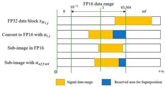
where $s_{M_{i,j_{max}}}$ represents the maximum absolute value in the data block, which can be quickly determined with the shared memory. In actual practice, this value usually can be freely selected within 65,504, which is the maximum of FP16.

In addition, to ensure that the superposition of the sub-images does not exceed the dynamic range of FP16, and to avoid the uneven grayscale in the final image, a specification factor ${\alpha }_{offset}$ is designed in this study, which is defined as:

$${\alpha }_{offset}=\frac{Nu}{{\alpha }_{max}}\times \frac{V}{Ls\times PRF}$$

(15)

where PRF represents the pulse repeat frequency; V represents the radar velocity; ${\alpha }_{max}$ represents the maximum value of the adaptive loss factors in total data blocks.

Based on Equations (3) and (14), the back projection equation performed for each data block in this scheme is Equation (16), and the adaptive data range control in back projection is shown in Figure 9.

$$g_{i,j}\left(x_m,y_n\right)=\int \frac{s_{M_{i,j}}\left[{\tau }_{mn}\left(\eta \right),\eta \right]}{{\alpha }_{i,j}}\exp (\frac{j4\pi R_{mn}}{\lambda })d\eta$$

(16)

where $g_{i,j}\left(x_m,y_n\right)$ represents the FP16 sub-image. The specific imaging region for each data block is presented in Equations (5) and (6).

Based on Equations (15) and (16), the final imaging result $f_{BP}\left(x_m,y_n\right)$ can be expressed as:

$$f_{BP}\left(x_m,y_n\right)={\displaystyle \sum }_i{\displaystyle \sum }_j{g}_{i,j}\left(x_m,y_n\right)\times {\alpha }_{i,j}\times {\alpha }_{offset}$$

(17)

In addition, for meeting the dynamic range of FP16 and FP32, the interpolation in back projection is changed from interpolation by time-delay to interpolation by distance in this study, and the preprocessing for __cosf() by $4\pi \left[\frac{R_{mn}}{\lambda }-int\left(\frac{R_{mn}}{\lambda }\right)\right]$ is adopted.

3.3. FBP Algorithm with FP16

The FP16 acceleration scheme of the BP algorithm has been described above. The FBP algorithm simply replaces the direct back projection of the BP algorithm with a polar coordinate projection of the sub-aperture and two-dimensional interpolation to obtain the final image. The principle of FP16 FBP scheme is basically the same as the FP16 scheme of BP. The FP16 sub-images in Figure 7 are replaced by the FP16 polar sub-images obtained from the sub-apertures, and the FP16 two-dimensional interpolation is added to the sub-image fusion for the FP16 overall acceleration process of FBP. The selection of loss factors is based on order-of-magnitude statistics and the data range of pulse superposition. Since the FBP algorithm does not change the principle that each grid point coherently superimposes the contribution of the pulse in a synthetic aperture time, the loss and specification factors are still chosen based on Equations (14) and (15).

According to the correspondence between streaming structure and sub-aperture mentioned in Section 2.2, Equations (8) and (10) in the FP16 scheme of FBP can be expressed as:

$$f_i\left({\rho }_i,{\theta }_i\right)=\int \frac{s_{M_i}\left[{\tau }_{{\rho }_i,{\theta }_i}\left(\eta \right),\eta \right]}{{\alpha }_i}\exp [\frac{j4\pi (R_{{\rho }_i,{\theta }_i}-{\rho }_i)}{\lambda }]d\eta$$

(18)

$$f_{FBP}\left(x,y\right)={\displaystyle \sum }_{i=1}^M\left[f_i\left({\rho }_{x_i},{\theta }_{y_i}\right)\times exp\left(j\frac{4\pi }{\lambda }{\rho }_{x_i}\right)\times {\alpha }_i\times {\alpha }_{offset}\right]$$

(19)

where ${\alpha }_i$ and $s_{M_i}$ represent the loss factor and the range compressed data of the ith sub-aperture, respectively.

The FP16 implementation of the sub-aperture back projection kernel in the FBP algorithm is the same as Figure 8, except that the range calculation is performed in the polar coordinate system and the final image of the sub-aperture is obtained without multiplying any factors and superposition with the previous data block. The polar sub-image fusion kernel of FBP is performed by replacing the FP32 two-dimensional interpolation in Figure 4 with FP16 interpolation. However, FP32 instruction __sinf() is still used in the interpolation because there is too much loss of precision with FP16 instruction. The interpolated data of each sub-aperture achieves phase compensation in FP16 and then multiplies the specification and loss factor to complete the FP16 superposition of different apertures. In this paper, in order to ensure the accuracy of angle calculation, the inverse trigonometric instructions involved in FBP and FFBP algorithms adopt FP64. Except the inverse trigonometric instruction, the GPU schemes are all carried out according to the instructions of FP32 or FP16 described in this paper.

3.4. Error Analysis and Applicable Conditions

This paper only analyzes the additional errors caused by the FP16 calculation and does not include the errors of the algorithm itself. Since the errors of the whole image and individual pixel point depend on the number of operations, the errors caused by the data precision of the FBP algorithm could be smaller than those of the BP algorithm. In this paper, the error results are given as an example of the FP16 scheme of BP.

The binary representation of floating-point numbers is divided into sign (s), exponent (i), and mantissa (m), and the precision of the data representation is determined by the mantissa of the data. FP32 contains 1 sign, 8 exponents, and 23 mantissas, while FP16 has only 5 exponents and 10 mantissas. The calculation of a floating-point number F can be expressed as:

$$F={\left(-1\right)}^s\times 2^{\mathrm{i}}\times \left(1+0.\mathrm{m}\right)$$

(20)

The high data representation error of FP16 makes it a necessary consideration in imaging. Taking 1024 as an example ($2^{10}$), its representation error is $2^{-13}$ in FP32, but $2^0$ in FP16. The back projection requires $N_{Ls}\times Nx\times Ny$ additions and multiplications. By assuming $N_{Ls}=Nx=Ny=N$, the absolute and relative error equations for the data calculation are as follows:

$$\epsilon \left({\sum }_{i=1}^n{x}_i\right)={\sum }_{i=1}^n\epsilon \left(x_i\right)$$

(21)

$$\epsilon \left({\prod }_{i=1}^n{x}_i\right)={\sum }_{i=1}^n\left[\left({\prod }_{\begin{array}{c}j=1\\ j\ne i\end{array}}^n{x}_j^{*}\right)\epsilon \left(x_i\right)\right]$$

(22)

$${\epsilon }_r\left({\sum }_{i=1}^n{x}_i\right)=\max \left[{\epsilon }_r\left(x_1\right),{\epsilon }_r\left(x_2\right),\dots \dots \right]$$

(23)

$${\epsilon }_r\left({\prod }_{i=1}^n{x}_i\right)\approx \sum _{i=1}^n{\epsilon }_r\left(x_i\right)$$

(24)

where $\epsilon \left(x_i\right)$ indicates the absolute error of data representation; $x_i$ indicates the true value of data; $x_j^{*}$ indicates the value after data representation; ${\epsilon }_r\left(x_{\mathrm{i}}\right)$ indicates the relative error of data.

According to Equations (21) and (22), it can be concluded that the absolute error of FP16 addition for the whole image in the above case reaches $N^3$, while the absolute error of FP32 is only $2^{-13}\times N^3$, and the error of multiplication can be even larger. Low precision data representation errors are unavoidable. The schemes in this paper consider the adaptive adjustment of the order of magnitude of the data, leading to most of the operations around $2^0$. As a result, the corresponding FP16 addition absolute error is reduced to $2^{-10}\times N^3$, and the multiplication error can be also effectively reduced. Moreover, from Equations (23) and (24), it can be seen that the relative error of addition and subtraction is determined by the relative error of the data representation. The FP16 also has a high relative error, while the relative error of multiplication is constantly superimposed. Compared to the absolute error, it is more difficult to reduce the relative error of FP16.

The loss analysis is provided below for each pixel point. In the BP algorithm, N additions and multiplications are required for each point. When the order of magnitude of the data reaches $2^0$, the absolute error of addition can also be reduced to $2^{-10}\times N$, exactly consistent with the above analysis. For the error due to the reduced interpolation precision, the reduced data precision gives more losses to sinc interpolation compared to linear interpolation as the former performs more low-precision operations.

Based on the above discussion, some illustrations of the FP16 schemes application in this paper are provided. Considering the dynamic range of the data, this scheme can achieve excellent results for airborne and onboard imaging. Due to the time consumption introduced by the loss factor determination mechanism, greater speedups can be achieved for data with many pulses and few pulse sampling points. The FP16 scheme is more suitable for processing more concentrated data. When the amount of data to be processed is the same, the reduction of $Nu$ results in fewer advantages for FP16 data copies and video memory. The pre-processing is required for the operations of extreme magnitudes, such as speed of light and pulse sampling interval.

4. Experiment

To explore the effectiveness achieved by FP16 schemes, the following eight schemes are realized: BP-CPU-FP64, FBP-CPU-FP64, FFBP-CPU-FP64, BP-GPU-FP32, FBP-GPU-FP32, FFBP-GPU-FP32, BP-GPU-FP16, and FBP-GPU-FP16. The parameters of the environment, simulation, and the experimental scene are listed in

Table 1. Environment specifications.

Parameters	Value
System	Windows 10 (×64)
CPU	AMD Ryzen 7 5800H
GPU	NVIDIA GeForce RTX 3060
Environment	MATLAB 2021, VS 2019, CUDA 11.3

and

Table 2. Simulation and experimental parameters.

Parameters	Value
Wavelength	0.03125 m
PRF	533.330793 Hz
V	154.195864 m/s
Band width	480 MHz
Pulse width	2.4 us
Sampling rate	548571428.571429 Hz
Nearest distance	23305.0 m

. The simulation uses a 3072×1024 echo volume with an upsampling factor of 2 to image a scene with an azimuth of 750 m and a distance of 250 m. The radar azimuth center is the origin. The motion direction is y-axis positive, the coordinate of the simulation point is (23,500 m, 4 m), the grid is divided as $7501\times 2501$ according to 0.1 m, the number of sub-aperture is 64, and each sub-aperture contains 48 pulses. For comparison, $Nu$ of BP schemes is also taken as 48. In this paper, the merge base of FFBP is chosen as 2, and the number of streams is set as 4. Each thread block in the kernel function contains 256 threads, and the number of thread blocks depends on the number of grid points required for the different kernel functions.

4.1. Simulation Results and Analysis

The normalized amplitude diagrams in range and azimuth direction of the three CPU schemes for a point target are shown in Figure 10, and the comparison of the peak sidelobe ratio (PSLR) and the integral sidelobe ratio (ISLR) for the point target is shown in

Table 3. Imaging indicators of the CPU schemes.

Direction	Parameters	BP-CPU-FP64	FBP-CPU-FP64	FFBP-CPU-FP64
Range	PSLR (dB)	−13.3085	−13.3535	−13.2633
	ISLR (dB)	−10.1937	−10.3197	−10.2047
Azimuth	PSLR (dB)	−13.1957	−12.7574	−13.4845
	ISLR (dB)	−10.2021	−9.8649	−9.7976

. By comparison, it can be found that the energy aggregation effects are basically the same. The time consumption of BP, FBP, and FFBP schemes in Figure 10 are 30,357,648 ms, 570,969 ms, and 2,140,093 ms, respectively, and the fast time-domain algorithms achieve a good speedup. When there are few aperture divisions, the FFBP computation is larger than that of FBP according to the computational volume derivation in Section 2, resulting in a faster speed of the FBP algorithm.

According to the GPU acceleration schemes of BP, FBP, and FFBP algorithms proposed in Section 2 and Section 3, the simulation results of each algorithm under FP32 and FP16 are given in Figure 11. It can be seen that the BP-GPU-FP32, BP-GPU-FP16, and FBP-GPU-FP32 schemes maintain suitable sinc function waveforms with low sidelobes, and the FBP-GPU-FP16 scheme has high azimuthal sidelobes, but the energy aggregation effect is still acceptable. The experimental conditions and the FP32 instructions used in the FFBP-GPU-FP32 and FBP-GPU-FP32 schemes are the same, but the FFBP-GPU-FP32 scheme has too much interpolation, and the point target simulation error is large. The experiments in this paper can reduce the error by increasing the division density and changing to high-precision instructions to make the imaging quality of FFBP-GPU-FP32 close to that of FFBP-CPU-FP64. However, it can lead to a decrease in acceleration efficiency and an increase in video memory usage, making it unnecessary to be further discussed. To illustrate the feasibility of the FFBP-GPU acceleration scheme proposed in Section 2.3, the FFBP-GPU-FP32+ scheme after changing to many high-precision instructions on top of FFBP-GPU-FP32 is supplemented in this section. The corresponding results are given in Figure 11.

This experiment satisfies the density dividing condition proposed in Section 2. In Figure 11, the time consumptions of FBP-GPU-FP32 and FFBP-GPU-FP32 are 602 ms and 1184 ms, respectively, which is shorter than the 1653 ms of BP-GPU-FP32. BP-GPU-FP16 takes only 918 ms, and FBP-GPU-FP16 takes even less time with 440 ms. These results indicate that the BP-GPU-FP16 and FBP-GPU-FP16 achieve considerable imaging performance in a much shorter period of time, and the latter is more efficient.

Table 4. Imaging indicators of the four GPU schemes.

Direction	Parameters	BP-GPU-FP32	FBP-GPU-FP32	BP-GPU-FP16	FBP-GPU-FP16
Range	PSLR (dB)	−13.3722	−13.3028	−13.5414	−13.2985
	ISLR (dB)	−10.2416	−10.2350	−10.0277	−10.2866
Azimuth	PSLR (dB)	−12.9271	−12.0809	−11.5352	−7.9673
	ISLR (dB)	−7.9891	−6.1871	−5.6912	−1.2428

shows the imaging indicators of the different schemes. It can be seen that BP-GPU-FP16 has better simulation quality, compared with the FBP-GPU-FP16 scheme.

In terms of real-time imaging, the total time and back projection time of the BP-GPU-FP32, BP-GPU-FP16, FBP-GPU-FP32, and FBP-GPU-FP16 schemes for different grid divisions with 3072×1024 data volume are shown in

Table 5. Speedup with GPU-FP16 schemes of different grid divisions.

Grid Division	BP-GPU- FP32 (ms)	BP-GPU- FP16 (ms)	Speedup	FBP-GPU-FP32 (ms)	FBP-GPU-FP16 (ms)	Speedup
$3001\times 1001$	289	164	$1.76\times$	122	113	$1.07\times$
$4501\times 1501$	617	348	$1.77\times$	180	151	$1.19\times$
$6001\times 2001$	1070	601	$1.78\times$	315	246	$1.28\times$
$7501\times 2501$	1653	918	$1.80\times$	602	440	$1.37\times$
$9001\times 3001$	2379	1318	$1.80\times$	1046	750	$1.39\times$

and Figure 12, respectively. The back projection of FBP and FFBP algorithms are divided into 2 and 3 kernel functions in Section 2.2 and Section 2.3, respectively. It can be seen that:

• The computational volume of the algorithm is mainly concentrated in the back projection part, and the efficiency improvement achieved by using lower precision in the back projection part directly improves the overall efficiency of the algorithm.
• As the grid division becomes denser, the acceleration ratio of the BP-GPU-FP16 scheme compared to the BP-GPU-FP32 scheme increases and reaches about 1.8 times. The reasons for this result are that the copy speed of FP16 data is faster; the more pixels reduce the time-consuming proportion of adaptive loss factors determination, but make the proportion of FP16 calculations increase.
• Under the same division, the acceleration ratio of FBP-GPU-FP16 is lower than that of the BP-GPU-FP16 scheme, because the FP16 interpolation of aperture fusion in back projection uses the __sinf() instruction of FP32 to guarantee the interpolation accuracy, and its FP32 distance calculation is also more complicated. As shown in Figure 12, the acceleration ratio becomes larger as the grid division becomes denser, indicating that this FP16 scheme is also more advantageous for large computational volumes.

4.2. Experiment Results

Figure 13 shows the results of the eight schemes for the region of 750 × 750 m² selected by 0.15 m interval for the experimental data with 3072×4096 data volume, and the local area of the pictures is intercepted and enlarged. The other conditions of the experiment are the same as the above simulation. In Figure 13 the transverse direction is azimuth. It should be noted that whether motion compensation is performed has almost no effect on the image quality of the BP algorithm. In this paper, linear trajectories are used for the imaging processing, and the results in Figure 13 are adjusted for overall contrast for presentation purposes, but the image quality analysis in Section 4.3 is still performed on the original images. It can be seen that the imaging results of FFBP-GPU-FP32 and FBP-GPU-FP16 are relatively worse, which are related to more interpolation operations and low data precision, and the focusing results of other images are not significantly different.

4.3. Analysis of Image Quality

To quantitatively analyze the imaging quality of different schemes, Equation (25) is applied to calculate the image entropy H of complex images for $Ny\times Nx$ pixel points:

$$H=-{\sum }_{m=1}^{Ny}{\sum }_{n=1}^{Nx}\rho \left(m,n\right)log\rho \left(m,n\right)$$

(25)

$$\rho \left(m,n\right)=\frac{{\left|x\left(m,n\right)\right|}^2}{Pow}$$

(26)

where $x\left(m,n\right)$ represents the pixel value; $Pow$ represents the total pixel power; $\rho \left(m,n\right)$ represents the proportion of power.

Generally, the lower image entropy means a better focusing effect of SAR images. In addition, the mean structural similarity index measure (MSSIM) and peak signal-to-noise ratio (PSNR) are selected as the evaluation criteria of grayscale image quality, with larger values representing less difference between the image and the real scene. The BP-CPU-FP64 imaging result is selected for reference, and the evaluation results of other schemes are given in

Table 6. Image quality.

	Entropy	MSSIM	PSNR
FBP-CPU-FP64	22.9657	0.9985	48.5118
FFBP-CPU-FP64	22.9997	0.9953	42.3074
BP-GPU-FP32	23.0708	0.9986	49.9150
FBP-GPU-FP32	23.1461	0.9952	46.1326
FFBP-GPU-FP32	23.2721	0.9885	43.2326
BP-GPU-FP16	23.1695	0.9940	44.8880
FBP-GPU-FP16	23.2964	0.9808	41.5353

. It can be seen that the overall imaging quality of the CPU-FP64 schemes is better because it uses FP64 to process the data. With the same processing precision, BP achieves better focusing results compared to FBP and FFBP. The latter two both use different degrees of approximation to improve the imaging efficiency based on the original BP. Notably, the BP-GPU-FP16 scheme achieves similar imaging quality as the FBP-GPU-FP32 scheme, but the imaging quality of FBP-GPU-FP16 is reduced. In Table 6, it can be seen that the image quality of FBP-GPU-FP16 is similar to that of the FFBP-GPU-FP32, but Figure 13h shows an acceptable visual quality because PSLR in Section 4.1 is not the only factor affecting image quality. Due to the imaging quality and time of FFBP-GPU-FP32, the FFBP-GPU-FP16 scheme is not explored in this paper.

4.4. Analysis of the Real-Time Performance

The imaging time comparison in Section 4.2 is given in

Table 7. Running time of the eight schemes.

Time (ms)	BP -CPU -FP64	FBP-CPU -FP64	FFBP-CPU -FP64	BP-GPU -FP32	FBP-GPU -FP32	FFBP-GPU -FP32	BP-GPU -FP16	FBP-GPU -FP16
Total	155,563,001	526,937	1,108,282	2295	548	807	1274	415
Back projection	155,561,267	522,515	1,100,532	2250	466	663	1218	360

. The time for reading data from the file, writing back to the file, and initializing some parameters is not included in this study. Similar to the simulation results, the fast time-domain algorithms achieve higher efficiency at various data processing precisions, and their CPU schemes achieve hundreds of times acceleration compared to the BP-CPU-FP64 scheme. The GPU-FP16 schemes realize considerable accelerations relative to GPU-FP32 schemes and thousands of times acceleration relative to the CPU-FP64 schemes. The FBP-GPU-FP16 scheme achieves the highest efficiency. Furthermore, the fast time-domain algorithms can continue to use other optimizations on GPU-FP32 schemes to increase its acceleration ratio relative to the BP-GPU-FP32 scheme.

The FP16 performance in RTX 3060 is the same as that of FP32, which can halve the imaging time in Table 7. In contrast, the FP16 performance in A100 can reach 77.97 TFLOPS, which is four times the FP32 performance. With the development of FP16 performance in GPU, the FP16 scheme in this study can achieve a higher acceleration.

4.5. Analysis of Video Memory Usage

The back projection is the main time-consuming part of the BP algorithm and utilizes the most video memory. In

Table 8. Occupancy analysis of video memory.

Parameters	BP-GPU-FP32-Non-Streaming	BP-GPU -FP32	FBP-GPU -FP32	FFBP-GPU -FP32	BP-GPU -FP16	FBP-GPU -FP16
Video memory	573.65 MB	393.65 MB	1125.49 MB	1013.43 MB	292.24 MB	663.87 MB

, compared to the GPU non-streaming FP32 scheme and BP-GPU-FP32 scheme in Section 4.2, the BP-GPU-FP16 scheme uses 50.9% and 74.2% of the first two, respectively, greatly relieving the pressure on the video memory under the experimental data. The FBP and FFBP algorithms are characterized by large video memory consumption due to the sub-aperture imaging method, which poses a challenge to the limited video memory of the GPU. It can be seen that the FBP-GPU-FP16 scheme proposed in this paper utilizes only 59.0% of the video memory of the FBP-GPU-FP32 scheme, but it is still larger than the BP-GPU-FP32 scheme, which is the price for the fast time-domain algorithm to achieve high efficiency.

In the future, strategies such as multi-GPU collaboration can be used to assign different GPUs to perform the range compression and back projection of FP16. By this method, the time and memory usage of the range compression and back projection are balanced to achieve better results.

5. Conclusions

In this study, an adaptive asynchronous streaming scheme for the BP algorithm and FBP algorithm based on FP16 is proposed. The experimental results show that these schemes can improve the imaging efficiency of the GPU FP32 schemes in RTX 3060 by 1× and 0.5×, respectively, with similar imaging quality. The usage of video memory is also significantly decreased. Moreover, the advantage of these schemes is more obvious when the calculation increases.

The development trend of GPU indicates that the performance of low-precision arithmetic will be continuously optimized, while the improvement of image quality obtained through high-precision arithmetic will be unnecessary due to its high resource consumption. Based on imaging quality, video memory usage, imaging speed, and the prospect of FP16 operation of GPU, the BP-GPU-FP16 and FBP-GPU-FP16 schemes proposed in this paper have advantages over the FP32 schemes.