Time Series Forecasting of Software Vulnerabilities Using Statistical and Deep Learning Models

Abstract

Software security is a critical aspect of modern software products. The vulnerabilities that reside in their source code could become a major weakness for enterprises that build or utilize these products, as their exploitation could lead to devastating financial consequences. Therefore, the development of mechanisms capable of identifying and discovering software vulnerabilities has recently attracted the interest of the research community. Besides the studies that examine software attributes in order to predict the existence of vulnerabilities in software components, there are also studies that attempt to predict the future number of vulnerabilities based on the already reported vulnerabilities of a project. In this paper, the evolution of vulnerabilities in a horizon of up to 24 months ahead is predicted using a univariate time series forecasting approach. Both statistical and deep learning models are developed and compared based on security data coming from five popular software projects. In contrast to related literature, the results indicate that the capacity of Deep Learning and statistical models in forecasting the evolution of software vulnerabilities, as well as the selection of the best-performing model, depends on the respective software project. In some cases, statistical models provided better accuracy, whereas in other cases, Deep Learning models demonstrated better predictive power. However, the difference in their performance was not found to be statistically significant. In general, the two model categories produced similar forecasts for the number of vulnerabilities expected in the future, without significant diversities.

1. Introduction

The size and complexity of modern software systems are constantly increasing. Additionally, the number of software vulnerabilities has significantly grown, leading to an increase in the security concerns expressed both by the end users and the software enterprises. The exploitation of software vulnerabilities can lead to important financial damages, which renders the need of decision makers to assess the security level of software products absolutely necessary. They need to determine (i) whether software systems along with their respective software components (e.g., packages, classes, methods) are vulnerable or not, (ii) the impact of potential vulnerability exploits, and (iii) the likelihood that a specific number of vulnerabilities will be reported in a certain period of time.

To deal with this, many researchers have proposed models capable of discovering vulnerabilities. A lot of effort has been placed on the prediction of vulnerable software components using software attributes extracted by the source code. In these studies, researchers commonly train machine learning models based on either software metrics (e.g., cohesion, coupling, and complexity metrics) [1,2,3] or text features [4,5,6,7]. They aim to identify patterns in the source code that indicate that a file or a function is vulnerable or not. However, these approaches do not predict the number of vulnerabilities in future versions. Although they assess whether a component contains vulnerabilities or not, they do not provide any indication of the evolution of the number of their vulnerabilities in time.

An indication of the expected number of vulnerabilities and the trends of their occurrences can be a very useful tool for decision makers, enabling them to prioritize their valuable time and limited resources for testing an existing software project and patching its reported vulnerabilities. For this purpose, there is a need for forecasting models that can predict the trend and the number of vulnerabilities that are expected to be discovered in a specific time horizon for a given software project. Studies that propose mechanisms to model the evolution of the number of vulnerabilities in time [8,9] aim not to detect vulnerabilities, but to forecast the number of vulnerabilities that are likely to be identified in the future. These studies utilize either statistical or machine learning algorithms in order to estimate the expected number of vulnerabilities based on the vulnerabilities that have been already reported (e.g., in the National Vulnerability Database [10]). The majority of these algorithms are time series models that keep track of all the vulnerabilities in terms of calendar time and interpret that time as an independent variable [11]. Statistical models such as Autoregressive Integrated Moving Average (ARIMA), Croston’s method, logistic regression, and exponential smoothing models have attracted the interest of the researchers in the field [12,13]. Machine Learning (ML) models have been considered as well. Jabeen et al. conducted a comparative analysis evaluating different statistical models with various ML models such as Support Vector Machines and Bagging [14].

Deep learning (DL) has emerged as a promising solution for time series forecasting, as well. Karasu et al. utilized the long short-term memory network in order to predict the crude oil price [15]. Altan et al. used DL and, more specifically, a hybrid model including the LSTM network for time series forecasting as well [16]. In their study, they focused on the prediction of the digital currency price through time. Recent studies have introduced DL models as predictors capable of modelling the evolution of the vulnerabilities number in time [12,17]. Despite the existing attempts, a lack in the literature of a thorough DL analysis for vulnerability forecasting was noticed. In fact, although the existing studies [12,14,18] use neural networks to forecast the vulnerabilities number, their predictive capacity has not been thoroughly studied. Gencer et al. [17] recently conducted a more in-depth analysis, by considering several DL algorithms; however, they focused only on Android systems. In addition to that, the authors did not follow a project-specific approach, i.e., they did not build models to predict the future number of vulnerabilities for each Android application, but they aggregated all the vulnerabilities relative to Android applications and attempted to provide forecast for their aggregated value. This way, their results cannot be generalised for the task of predicting the number of vulnerabilities of a software project in a future version.

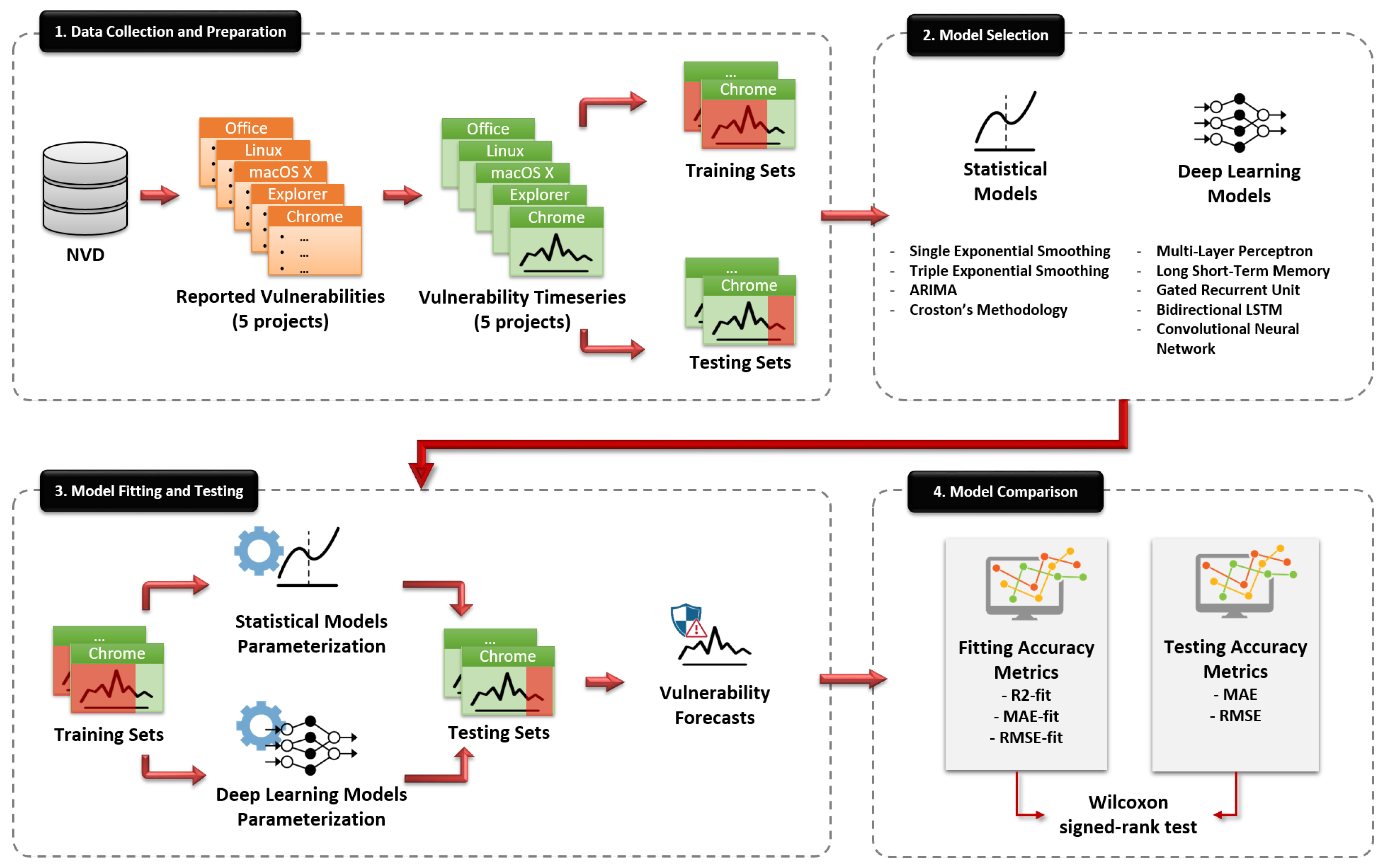
To this end, in the present paper we empirically examine the capacity of statistical and DL models in forecasting the number of vulnerabilities that a software product may exhibit in the future and we compare their predictive performance. For this purpose, we utilize data provided by the National Vulnerability Database (NVD) that provides files with the reported vulnerabilities of several software products. We gathered data about the reported vulnerabilities of five popular software applications, which have been reported in the last two decades (i.e., from 2002 to 2022), and, based on these data, we build several statistical and DL models for each one of the five projects, for providing vulnerability forecasts in a horizon of 24 months ahead. The produced models are evaluated and compared based on their goodness-of-fit, as well as on their predictive performance on unseen data. To the best of our knowledge, this is the first study that thoroughly evaluates the capacity of DL models in vulnerability forecasting and compares their predictive performance with traditional statistical models, in an attempt to emerge the DL models as adequate predictors of the future number of software vulnerabilities’ occurrences.

The contribution of our work is summarized in the followings:

• An in-depth examination of DL models as a method for forecasting the number of vulnerabilities that a software project will contain in the future.
• A comprehensive comparison between DL and statistical models in vulnerability forecasting.
• A methodology for forecasting the number of vulnerabilities related to an individual future timestep, instead of predicting the cumulative number of vulnerabilities until that timestep.

To sum up, in comparison with the state-of-the-art approaches, our contribution is primarily that we proceeded to the first thorough investigation of the capacity of DL in forecasting the number of vulnerabilities for a specific project in a future timestep, and subsequently that we performed an in-depth comparison between statistical and DL methods for the task of vulnerability forecasting. Most studies in the field examine traditional statistical time-series models [8,9,11,13] while few of them also examine ML models [12,14] or they just include in their analysis a kind of neural network, without proceeding with an in-depth analysis of DL models [12]. The only known work being closely related to ours that attempts to address the aforementioned issues is the work conducted by Gencer et al. [17]. However, contrary to Gencer et al. [17] who focused on the vulnerabilities of Android applications and built DL models that forecast the future evolution of the number of vulnerabilities in Android applications in general (by accumulating the vulnerability reports of all the studied Android applications), we provide a project-specific approach in which we build a different forecasting model for each one of the studied software projects. In addition to this, as opposed to Gencer et al. [17], we do not focus on a specific programming language. Finally, contrary to the approaches of [11,14], we do not predict the accumulative number of vulnerabilities until a timestep, but instead we try to predict the exact number of vulnerabilities that will occur in that specific future timestep.

The rest of the paper is structured as follows. In Section 2, the related work in the field of Vulnerability Forecasting in software systems is presented. Section 3 provides information about the proposed models, the overall methodology and the experimental setup. Finally, Section 4 thoroughly discusses the obtained results of our analysis, while Section 5 sums up the paper, provides the overall conclusion and also discusses potential future research directions.

2. Related Work

Examination of previous studies in the literature regarding vulnerability prediction shows that approaches based on statistics, mathematical modeling, and ML have been used. Code attribute-based models and time series-based models are the two primary categories of these approaches. The models based on code attributes concentrate on identifying the relationship between code attributes and the existence of vulnerabilities. On the other hand, time series-based models focus on predicting the number of vulnerabilities in a future time step based on historical data.

Regarding the code-based models, Automated Static Analysis (ASA) is often used for the early identification of security issues in the source code of software projects [19,20]. ASA manages to identify potential security threats that reside in the source code, by applying some pre-defined rules and identifying the violations of these rules. Based on ASA, more advanced models have been also proposed [21]. Siavvas et al. proposed a model that combines low-level indicators (i.e., security-relevant static analysis alerts and software metrics) in order to generate a high-level security score that reflects the internal security level of the examined software [21].

Apart from ASA, for the prediction of vulnerabilities in the source code the research community has widely employed ML and DL algorithms that try to identify code patterns or code attributes relative to the existence of vulnerabilities. Shin and Williams [1,2] examined how well software metrics, in particular complexity metrics, can predict software vulnerabilities. Several regression models were developed to differentiate between vulnerable and non-vulnerable functions. The effectiveness of feeding artificial neural networks with software measures to anticipate cross-project vulnerabilities was examined by the authors in [22]. Several ML models were developed, evaluated, and compared using a dataset of popular PHP products.

Neuhaus et al. proposed Vulture [6], a vulnerability prediction model that identified vulnerabilities based on import statements and function calls that are more frequent in vulnerable components. In VulDeePecker [5], Li et al. proposed a DL model for vulnerability identification. They separated the original code into several lines of code that were semantically connected, and then they used word2vec embeddings [23,24] to turn those lines of code into vectors. Subsequently, a neural network was trained to identify library/API function calls associated with known defects. In [25], the authors compared text mining and software metrics approaches using several machine and DL models for vulnerability prediction and then they attempted to combine these two approaches, as well. The aforementioned code-based models are categorized in

Table 1. Code-based models’ discrete characteristics.

Code-Based Model	Characteristics	Referenced Papers
Static analysis-based	Pattern-matching method. It checks violations of pre-defined rules.	[19,20,21]
Software metrics-based	ML algorithms that utilize software attributes as input.	[1,2,22,25]
Text mining-based	ML algorithms that process textual tokens that reside in the source code instead of numerical metrics.	[5,6,24,25]

.

Regarding the time series-based models, Alhazmi et al. proposed a time-based model [11]. Their approach is based on the fact that interest in newly released software rises in the beginning, peaks after a while, and then drops as new competitive versions are introduced. Yasasin et al. examined the issue of estimating the quantity of software security flaws in operating systems, browsers, and office applications [18]. They retrieved their data from NVD and they used mainly statistical models such as ARIMA and exponential smoothing. They also investigated the suitability of the Mean Absolute Error (MAE) and the Root Mean Square Error (RMSE) in the measurement of vulnerability forecasting. Furthermore, Jabeen et al., conducted an empirical analysis, where they compared different statistical algorithms with ML techniques showing that many of the ML models provide better results [14]. Shukla et al. in their study [26] attempted to include in their model the so called change point in order to assimilate the information about the time point when changes in the code size, popularity or known vulnerabilities can cause changes in the time series distribution. Wang et al. attempted to include the effort factor (i.e., any factor that can depict environmental changes of the software) in their cumulative vulnerabilities discovery model in order to predict trends in the vulnerability time series data [27]. In

Table 2. Time series-based models’ discrete characteristics.

Time Series-Based Model	Characteristics	Referenced Papers
Statistical models	Statistical models such as ARIMA and exponential smoothing, which predict the future number of vulnerabilities over a time period.	[8,9,12,13,14,17,18]
ML models	ML models that attempt to learn the number of vulnerabilities evolution through time, based on previous knowledge.	[12,14]
DL models	DL models (i.e., deep neural networks, recurrent neural networks, etc.) that attempt to learn the number of vulnerabilities evolution through time, based on previous knowledge.	[12,17]
Alhazmi–Malaiya model	A time-series model that attempts to predict the cumulative number of vulnerabilities until a specific time step.	[11]

, there is a list of the categories of the time series-based models.

In this study, we propose an approach to predict the evolution of vulnerabilities in an horizon of two years (i.e., 24 steps) ahead using both statistical and DL models. Actually, we compare these two kinds of time series models. We follow a univariate approach, considering only the number of the already reported vulnerabilities in the NVD regarding two operating systems, two browsers and one Office product (see Section 3.1). To the best of our knowledge, it is the first study that thoroughly examines the capacity of DL in forecasting the evolution of software vulnerabilities. While Gencer et al. [17] also compared the ARIMA with several DL models, their work focused solely on Android vulnerabilities by considering Android as a whole. In contrast, we follow a project-specific approach (i.e., specific browsers, operating systems) in order to be in line with a real-world scenario where a decision maker would desire to know the expected number of vulnerabilities for his/her product. We are also differentiated from the [11,14] approaches, as we attempt to predict the exact number of vulnerabilities until a specific month instead of the cumulative number of vulnerabilities until that month.

3. Methodology and Experimental Setup

In this section, a detailed description of the overall methodology of this study is presented. We analyze the data collection process, the parameters selection for our models, the training of the models and also the metrics that constitute the base of our evaluation process. In Figure 1, a chart that includes all the aforementioned steps is presented. All these steps are described in detail in the following sections.

3.1. Data Collection

The data used in the present study are collected from the publicly available American National Vulnerability Database (NVD). The NVD is a vulnerability database formed and maintained by the National Institute of Standard and Technology (NIST) of the US, which provides a comprehensive list of unique vulnerability and exposure data. The widespread contribution, public availability, and completeness of its security vulnerability information make it the most preferred vulnerability database in the related literature.

For the purposes of this work, we selected five popular software projects, namely Google Chrome, Microsoft Internet Explorer, Apple macOS X, Ubuntu Linux, and Microsoft Office. As regards our selection criteria, we based our decision on the fact that these projects represent popular categories of software systems, namely web browsers, operating systems, and office tools. Furthermore, we tried to maintain a balance between open- and closed- source software. Finally, these projects have been extensively used in the related literature for vulnerability analysis, prediction, and forecasting tasks [12,13,14,18]. After selecting the software projects covered in our analysis, we proceeded with collecting their corresponding vulnerability datasets from the NVD repository, starting from the first day of their release up until the latest available record by the end of 2021. Since the objective of our work is to forecast future security vulnerabilities, similarly to previous related studies, we grouped the available data (i.e., number of reported vulnerabilities) for each project in monthly intervals.

Table 3. Selected software systems and their descriptive statistics.

Software Project	Domain	Release Date	Open Source	Data Collection Period	Total Vulnerabilities
Google Chrome	Browser	2008	Partially	2008–2021	2136
Internet Explorer	Browser	1995	No	1997–2018	1039
Apple macOS X	OS	2001	No	2001–2021	2175
Ubuntu Linux	OS	2004	Yes	2005–2021	361
Microsoft Office	Office	1990	No	1999–2021	347

lists the selected software projects, accompanied with additional information, such as the total number of vulnerabilities and data collection period.

Figure 2 presents the number of monthly vulnerabilities for the five selected vulnerability datasets along with the software projects’ evolution.

3.2. Time Series Modelling

In line with previous related work on vulnerability forecasting [12,17,18], we follow a multiple forecasting approach, in which we compare several forecasting methodologies and evaluate their performance in terms of forecasting accuracy. More specifically, we fit various forecasting models on the five obtained time series datasets of monthly security vulnerabilities and subsequently, we evaluate the results against a test set of held out security vulnerability data. To do so, we employ and examine two main types of forecasting methodologies, ranging from simple statistical methods to more sophisticated DL approaches. Statistical forecasting methods comprise single and triple exponential smoothing (SES, TES) models, Autoregressive Integrated Moving Average (ARIMA) models, and Croston’s methodology. On the other hand, DL, i.e., Neural Network-based approaches, comprise models such as the Multi-Layer Perceptron (MLP), the Recurrent Neural Network (RNN) and its several variants, as well as the Convolutional Neural Network (CNN). Similar statistical and DL approaches have been widely used in both practice and academia for software quality evolution modelling and forecasting tasks [28,29,30,31,32,33], and more recently for predicting the future evolution of software vulnerabilities [12,13,14,17,18].

Since the objective of this study is to investigate various forecasting methodologies for their ability to predict the future evolution of software security vulnerabilities, we define our dependent variable as the number of vulnerability occurrences at each time interval. As mentioned previously, the number of vulnerabilities is aggregated by month, and time is measured in terms of month and year. Our focus lies on univariate time series modelling, meaning that the models will try to predict the number of vulnerabilities that will be reported for a given project in a future point in time, based exclusively on past observations of the number of reported vulnerabilities, without utilizing any additional feature.

In what follows, we provide a brief description of the forecasting methods that will be used in the context of this work for vulnerability forecasting. More specifically, in Section 3.2.1 we give an overview of the statistical models that we built as part of the present study, whereas in Section 3.2.2 we present the DL models examined in this study.

3.2.1. Statistical Models

While there are several forecasting methods that could be used for vulnerability forecasting, such as Artificial Neural Networks (ANNs), Support Vector Regression (SVR), or Regression Trees (RT), the application of these methods usually requires extensive parameter tuning and computational power. Therefore, as an initial approach towards vulnerabilities forecasting we decided to investigate statistical models that are generally more straightforward, less computationally expensive, and less data demanding. More specifically, our statistical models’ set comprises four widely used models, namely single exponential smoothing (SES), triple exponential smoothing (TES)—also known as Holt–Winters model, Autoregressive Integrated Moving Average (ARIMA), and finally, Croston’s methodology.

Starting with the single exponential smoothing (SES), this simple model produces forecasts by essentially using weighted averages, where the weights decrease exponentially as observations lie further in the past. In other words, the more recent the observation the higher the associated weight. To adjust the magnitude of the weights, a smoothing parameter alpha ($\alpha$) can be used, with smaller values of a giving more weight to the observations from the more distant past. Since SES only depends on the linear parameter $l_t$, i.e., the level of the series at the last observation at time t, it has a “flat” forecast function, meaning that every step into the future is predicted with the same value ${\widehat{y}}_{t+h|t}$. Due to this limitation, this model is suitable only for univariate data without a clear trend or seasonality patterns. The output of the SES is described in the following equation:

$$\begin{array}{c}\hfill {\widehat{y}}_{t+h|t}={\widehat{y}}_{t+1|t}=l_t\\ \hfill l_t=\alpha y_t+(1-\alpha )l_{t-1}\end{array}$$

(1)

Triple exponential smoothing (TES), also known as Holt–Winters exponential smoothing, is an extension of exponential smoothing that explicitly adds support for trend and seasonality to the univariate time series. In addition to the alpha ($\alpha$) smoothing factor, two new parameters called beta ($\beta$) and gamma ($\gamma$) are added to the equation. Parameter $\beta$ can be used in order to add the trend component $b_t$ to the outcome variable, denoting the slope of the time series at time t. In a similar way, a parameter ($\gamma$) acts as a weight that controls the influence on the seasonal component $s_t$ over the m most recent time periods. The output of the TES is described in the following equation:

$$\begin{array}{c}\hfill {\widehat{y}}_{t+h|t}=l_t+h{b}_t+s_{t+h_m-m}\\ \hfill l_t=\alpha (y_t-s_{t-m})+(1-\alpha )(l_{t-1}+b_{t-1})\\ \hfill b_t=\beta (l_t-l_{t-1})+(1-\beta )b_{t-1}\\ \hfill s_t=\gamma (y_t-l_{t-1}-b_{t-1})+(1-\gamma )s_{t-m}\end{array}$$

(2)

where $h_m=\left[(h-1)modm\right]+1$, to ensure that the estimates of the seasonal parameters are correct. There are two variations to this method with respect to the seasonal component, namely the additive and multiplicative method. The former is used when the seasonal variations are constant over time, while the latter is preferred when the seasonal variations are changing proportional to the level of the series.

A different, yet widely-used approach to time series forecasting are the Autoregressive Integrated Moving Average (ARIMA) models, introduced by Box and Jenkins to deal with the modeling of non-stationary time series [34]. While exponential smoothing models try to model the trend and seasonality patterns in the data, ARIMA models focus on describing the autocorrelations in the data. The ARIMA models are parameterized by adjusting three distinct integers: p, d and q. Parameter p represents the autoregressive (AR) part of the model, i.e., regression of the time series onto itself. Parameter d stands for the integrated (I) part of the model and incorporates the amount of differencing (i.e., the number of past time points to subtract from the current value) to apply to the time series for becoming stationary. Parameter q is the moving average (MA) part of the model. To estimate the three ARIMA parameters, the Box and Jenkins ARIMA modelling strategy involves four steps: Identification, Estimation, Diagnostic testing, and Application. When seasonality is present in the data, a Seasonal ARIMA, i.e., an extension of ARIMA that explicitly supports seasonal component can be formed by including three additional parameters, namely P, D and Q. These parameters are similar to the non-seasonal ARIMA components, but focus on the seasonal component. The general ARIMA(p,d,q) model is described in the following equation:

$$\begin{array}{c}\hfill {\widehat{y^{\prime }}}_{t+h|t}=c+{\Phi }_1{y}_t^{\prime }+{\Phi }_2{y}_{t-1}^{\prime }+...+{\Phi }_p{y}_{t-p}^{\prime }+{\theta }_1{e}_{t-1}+{\theta }_2{e}_{t-2}+...+{\theta }_q{e}_{t-q}+e_t\end{array}$$

(3)

where c is a constant, ${\Phi }_p$ are the coefficients of the autoregressive model, $e_t$ is a zero mean white noise error factor, and ${\theta }_q$ forms the moving average terms.

An inherent characteristic of vulnerability evolution datasets is that they are mostly zero-inflated and intermittent, meaning that they contain a lot of zero values and show a high volatility when a value occurs. To tackle the challenge of forecasting such time series, Croston proposed a solution, also known as Croston’s method [35]. Croston’s method involves the decomposition of the original time series into two new time series, one without zero values (${\widehat{z}}_{t+h|t}$) and a second one that captures duration of zero valued intervals (${\widehat{v}}_{t+h|t}$). Subsequently, to produce forecasts, separate simple exponential smoothing models are used to model the two new series, using again the alpha (a) smoothing parameter (identical to both series) to adjust the weights. Therefore, Croston’s methodology is also covered within the context of this study to investigate whether it can address the specific nature of security vulnerability time series data. It is described in the following equation:

$$\begin{array}{c}\hfill {\widehat{y}}_{t+h|t}=\frac{{\widehat{z}}_{t+h|t}}{{\widehat{v}}_{t+h|t}}\\ \hfill {\widehat{z}}_{t+h|t}=\left\{\begin{array}{cc}{z}_t\hfill & \mathrm{if}{y}_t=0\hfill \\ \alpha y_t+(1-\alpha )z_t\hfill & \mathrm{if}{y}_t\ne 0\hfill \end{array}\right.\\ \hfill {\widehat{v}}_{t+h|t}=\left\{\begin{array}{cc}{v}_t\hfill & \mathrm{if}{y}_t=0\hfill \\ \alpha y_t+(1-\alpha ){\widehat{y}}_t\hfill & \mathrm{if}{y}_t\ne 0\hfill \end{array}\right.\end{array}$$

(4)

3.2.2. Deep Learning Models

In this section, a brief description of the DL models that are utilized in this work is following. DL models are commonly based on artificial neural networks that are computational models with numerous processing components that take inputs and produce outputs in accordance with their predetermined activation functions. In this study, we investigate the time series forecasting capacity of the Multi-Layer Perceptron (MLP), the Recurrent Neural Network (RNN) and its several variants as well as the Convolutional Neural Network (CNN). As an instance, the following equation presents the formula describing a neural network’s output:

$${\widehat{y}}_{t+h|t}=b_o+\sum _{i=1}^I{b}_{i}g(k_{0j}+\sum _{j=1}^J{k}_{ij}{p}_j)$$

(5)

where $b_i$ are the weights of the network for the output and $k_{ij}$ are the neural networks weights for the hidden layers. J stands for the number of observation used as input $p_j$. The $b_0$ and $k_{0j}$ are the biases of each neuron. I is the number of hidden nodes in the network and g is a non-linear activation function.

Starting with the MLP, it is a feed-forward artificial neural network (ANN) that is made up of many perceptron layers. In particular, the MLP is frequently used in deep learning to build Deep Neural Networks (DNNs), which are ANNs with a lot of hidden layers between the input and output layer. The values of some particular variables known as hyperparameters determine the overall training process of an ANN and, in turn, of an MLP.

The most disseminated category of DNNs for data in the form of sequences (as happens with time series data) are the RNNs. Unlike the feed-forward neural networks, the RNNs are capable of processing entire sequences of data such as text features or time series data. Their speciality lies in the fact that the output is not only affected by the weights applied to the inputs, as in the case of traditional ANNs, but is also affected by a hidden state vector which contains information about the previous inputs. Thus the same input can give a completely different result depending on the previous inputs that are part of the sequence. In feed-forward ANNs, information flows from the input layer to the output layer through the hidden layers. It does not pass through a node twice. That is why they have no memory. However, in RNNs, the information forms a cycle. When the RNN makes a decision, it takes into account the current input and what it has learned from the inputs that it has previously received.

However, long data sequence learning is difficult for RNNs due to the issue of vanishing gradients [36]. When the gradient decreases further, the updates of the parameters become insignificant and no actual learning is performed. The so-called Long-Short Term Memory (LSTM) neural networks [37] give a solution to the problem of vanishing gradients. LSTMs networks are an extension of the simple RNNs and have the ability to learn from sequences with a very large number of time instants. This is because LSTM modules contain their information in a memory like the computer memory. Actually LSTMs can read, write and erase information from their memory. The LSTM learns over time which information is important and which is not. From an architectural view, the LSTM includes three gates, the input gate, the output gate and the forget gate. The input gate decides what new information will be stored in the LSTM’s memory, the output gate decides what information will affect the output at the current time, while the forget gate erases information that it considers unimportant.

Later, the Gated Recurrent Unit (GRU) model was devised. Like the LSTM, it can overcome the vanishing gradient obstacle [38]. It is actually a variant of the LSTM that contains two gates, the update gate and the reset gate. The difference with LSTM is that the processes of the input and forget gates are handled by one gate, the update gate. Another RNN variant, the bidirectional LSTM, known as biLSTM [39], is a sequence processing model that consists of two LSTMs, one of which receives input forward and the other of which receives input backward. With the help of BiLSTMs, the network has access to more information, which benefits the algorithm’s context (e.g., knowing what values immediately follow and precede a value in a sentence).

Convolutional Neural Networks (CNNs) [40] are often reliable when dealing with sequential and time series data, as well. One-dimensional CNNs can be used for univariate time series forecasting even though CNNs were originally designed for two-dimensional image data. An one-dimensional CNN model is a neural network with one convolutional hidden layer that operates over an one-dimensional sequence and can be followed by (at least) a second convolutional layer, when there are very long input sequences. After the hidden layers, there is a pooling layer tasked with reducing the output of the convolutional layers to its most important components. Subsequently, the feature maps that are extracted by the convolutional part of the network are flattened in order to reduce their dimension to a single one-dimensional vector. This one-dimensional network is given to a dense layer that is fully connected and produces the forecasted value based on the selected loss function.

3.2.3. Accuracy Metrics

In the literature, two of the most common categories of accuracy metrics when dealing with forecasting tasks are the absolute metrics, such as the mean absolute error (MAE) or root mean square error (RMSE), and the percentage-error metrics, such as the mean absolute percentage error (MAPE) [41]. However, as this study deals with zero-inflated time series, percentage-error metrics (such as the MAPE) are not appropriate, since their formula has the disadvantage of producing infinite or undefined values for zero or close-to-zero actual values, resulting to division by zero problems [42].

Therefore, in line with other related studies on vulnerability forecasting [12,14,17,18], we evaluated and compared the predictive performance of the investigated models using absolute metrics, and more specifically the Mean Absolute Error (MAE) as well as the Root Mean Square Error (RMSE). Both of these error metrics are widely used in forecasting tasks and can accurately reflect the performance of models fitted on zero-inflated time series. MAE measures the average magnitude of the errors in a set of predictions, without considering their direction. RMSE is a quadratic scoring rule that also measures the average magnitude of the error. Both MAE and RMSE express average model prediction error in units of the variable of interest and therefore can be easily interpreted. The equations of MAE and RMSE are given below:

$$MAE=\frac{{\sum }_{i=1}^n|y_i-\widehat{y_i}|}{n}$$

(6)

$$RMSE=\sqrt{\frac{1}{n}\sum _{i=1}^n{(y_i-\widehat{y_i})}^2}$$

(7)

where n is the number of observations, $y_i$ is the actual value and $\widehat{y_i}$ is the forecast value.

In addition to the selected predictive-power metrics introduced above, we also employ the $R^2$ coefficient of determination in order to measure the goodness-of-fit of the investigated models, i.e., how well the models fit on the data that were used during training. The $R^2$, which represents the square of correlation between the dependent and independent variables, is a statistical measure that shows how close the data fit to the regression line. Its formula is calculated as follows:

$$R^2=1-\frac{{\sum }_{i=1}^n{(y_i-\widehat{y_i})}^2}{{\sum }_{i=1}^n(y_i-\widehat{y_i})}$$

(8)

where $y_i$ is the actual value and $\widehat{y_i}$ is the forecast value. $R^2$ values close to 1 indicate an extremely good fit, whereas smaller values show a poor or no fit.

3.3. Fitting Time Series Models

This section describes the methodology followed in order to build the various statistical and DL models that were introduced in Section 3.2, with the purpose to fit and model the vulnerability evolution of the five vulnerability datasets (i.e., software projects). As a first step, we defined monthly periodicity for all datasets and subsequently we proceeded with model parameterization. As mentioned in Section 3.2, in this work we followed a train-test split approach. More specifically, each of the five vulnerability datasets was split into two parts, where the first n-24 observations were used for model fitting, and the last 24 observations (i.e., 24 months) were used as held-out vulnerability data for testing and evaluating the model performance on unseen data. The model parameterization and fitting processes described in the rest of this section were performed solely on the training parts of the datasets. Goodness-of-fit (i.e., training) results that were obtained through fitting the models on the five selected software projects, as well as results on the held-out (i.e., testing) data are presented and discussed later, in Section 4.

3.3.1. Statistical Models

In this subsection, we focus on describing the fitting and parameterization process concerning the four selected statistical models covered in our study, i.e., SES, TES, ARIMA and Croston methodology. Starting with the simplest model, namely SES, there is not much tuning to be done, since the only parameter is the smoothing factor alpha (a). We employed the StatsModels [43] library, a Python module that provides functionality for the estimation of many different statistical models, in order to automatically estimate model parameters for each dataset by maximizing the log-likelihood. Column “a (level)” in

Table 4. Optimal parameters for exponential smoothing models.

Software Project	a (Level)	$\mathit{\beta }$ (Trend)	$\mathit{\gamma }$ (Seasonal)
Google Chrome	0.129	0.000	0.000
Internet Explorer	0.179	0.000	0.256
Apple macOS X	1.922 × 10${}^{-8}$	6.891 × 10${}^{-13}$	4.383 × 10${}^{-9}$
Ubuntu Linux	0.247	0.000	0.000
Microsoft Office	0.052	7.362 × 10${}^{-15}$	2.256 × 10${}^{-12}$

lists the optimal SES (a) parameter value for each vulnerability dataset. Similarly to SES, we employed the StatsModels library in order to also estimate the optimal beta ($\beta$) and gamma ($\gamma$) parameters of the TES models for each time series dataset. As explained earlier, parameter $\beta$ can be used in order to add the trend component to the outcome variable, while parameter $\gamma$ controls the influence on the seasonal component. Since our time series are zero-inflated, we chose the additive method. Columns “$\beta$ (trend)” and “$\gamma$ (seasonal)” of Table 4 list the optimal TES ($\beta$ and $\gamma$) parameter values for each vulnerability dataset.

After fitting the optimal SES an TES models, we proceeded with the more sophisticated ARIMA methodology. A fundamental assumption in ARIMA analysis is stationarity, i.e., the statistical properties (such as mean and variance) of a time series need to be constant over time. Therefore, the first step towards our analysis included stationarity checks. We used time series decomposition to deconstruct each time series dataset into several components, representing one of the underlying categories of patterns, i.e., trend, seasonality, and residual components of the data. By inspecting the decomposition plots, we observed that in all covered cases, the seasonal component and the decreasing trend of the data were nicely separated, leading to the conclusion that the series are not stationary in nature and need to be adjusted in order to satisfy the necessary assumptions. The most common practice for making a series stationary is to transform it through differencing. To verify that a first-order difference would make the series stationary, we proceeded with all the required steps, such as Auto-Correlation Function (ACF) correlograms analysis, as well as Dickey–Fuller tests [44], which tests the null hypothesis that a unit root is present in an autoregressive model. Detailed results of the Dickey–Fuller tests on the data after applying a first-order difference are presented in

Table 5. Dickey–Fuller test on first-order differenced data.

Software Project	Test Statistic	p-Value	Critical Value (1%)
Google Chrome	−6.267	4.087 × 10${}^{-8}$	−3.475
Internet Explorer	−4.762	0.0098	−3.460
Apple macOS X	−7.021	6.550 × 10${}^{-10}$	−3.459
Ubuntu Linux	−6.897	1.310 × 10${}^{-9}$	−3.468
Microsoft Office	−7.529	3.604 × 10${}^{-11}$	−3.457

.

For a time series to pass the Dickey–Fuller stationarity test, the “Test Statistic” value should be lower than the “Critical Value”. Table 4 indicates that after applying a first-order difference, the five examined time series become stationary, as the Test Statistic values are lower that the Critical Values in all cases. This is also confirmed by inspecting the significance of p–values (p < 0.05). Since the number of required transformations to make a time series stationary corresponds to the d parameter of the ARIMA(p,d,q) model [34], setting the value of $d=1$ for each model corresponding to the investigated datasets can be safely supported by the above analysis.

As a next step, we aimed to identify the p (AR), q (MA), P (seasonal AR), and Q (seasonal MA) parameters of the ARIMA models for each dataset, following the practical recommendations through visual inspection of the AutoCorrelation Function (ACF) and Partial AutoCorrelation Function (PACF) correlograms [34] of the first-order differenced time series. Based on practical recommendations, if the ACF of the series disappears gradually, and the PACF of the series disappears abruptly, it indicates an AR component. An opposite behavior, i.e., the ACF disappears abruptly and the PACF disappear gradually, indicates an MA component. In addition, if the ACF of the differenced series is positive at lag s, where s is the number of periods in a season, it indicates a seasonal AR term, while a negative ACF at lag s indicates a seasonal MA term.

When no clear conclusion can be reached by inspecting the ACF and PACF correlograms, we turn towards the Akaike Information Criterion (AIC) minimization. For this purpose, we employed the AutoArima library [45], a Python module that provides functionality for identifying the optimal parameters for an ARIMA model based on a given information criterion (e.g., AIC). Experiments were conducted by assigning various combinations of values (between 0 and 5) to the pq, P, and Q parameters, while keeping the d parameter equal to 1.

Table 6. Optimal parameters for ARIMA models.

Software Project	Order (AR, I, MA)	Seasonal Order S (AR, I, MA, m)
Google Chrome	(5, 1, 3)	(1, 0, 0, 12)
Internet Explorer	(2, 1, 4)	(1, 0, 1, 12)
Apple macOS X	(2, 1, 5)	(1, 0, 1, 12)
Ubuntu Linux	(1, 1, 2)	(1, 0, 0, 12)
Microsoft Office	(2, 1, 2)	-

provides details on the optimal parameters for ARIMA models for each time series dataset, as identified using the above recommendations through manual inspection and automated processes.

In time series analysis, it is a common practice to include a random walk model for the purpose of comparing it with the selected models. The random walk model excludes the auto-regressive (AR) and moving average (MA) parameters. Therefore, in the experiments presented in the Section 4 we have also included ARIMA (0, 1, 0) as our baseline random walk model.

Finally, regarding Croston’s methodology, we used Mohammadi’s python implementation [46] which also automatically optimises parameters on the training set. However, this implementation does not provide APIs for returning the optimal parameters of the fitted model, so we were not able to retrieve and list them within the context of this work.

3.3.2. Deep Learning Models

Data Transformation

In this section, we examine the capacity of the DL models to fit and model the evolution of the number of reported vulnerabilities through time. In a similar way with the statistical models, we consider as time intervals the monthly observations of the reported vulnerabilities. For the purposes of training and evaluating our models we utilized the five software products that we selected (see Section 3.1). We followed the train-test split approach, where we used the first n-24 months to train our models and the rest (unseen during the training phase) 24 months as a test-bed to compute the accuracy metrics.

As we perform a multi-step forecasting for a period of 24 time steps (i.e., months), we take full advantage of the ability of neural networks to produce many outputs at once. In other words, the models that we developed perform multi-output regression and predict the entire forecast sequence in a single instance. The following equation describes this process for an example of a three-step forecast, where a model predicts the dependent variable for three steps ahead based on the knowledge of the last n observations.

$$\mathrm{prediction}\left(\mathrm{t}\right),\mathrm{prediction}(\mathrm{t}+1),\mathrm{prediction}(\mathrm{t}+2)=\mathrm{model}\left(\mathrm{obs}\right(\mathrm{t}-1),\mathrm{obs}(\mathrm{t}-2),\dots ,\mathrm{obs}(\mathrm{t}-\mathrm{n}\left)\right)$$

(9)

As already stated, the goal of multi-output regression is to predict two or more numerical values. In contrast to normal regression where a single value is predicted for each sample, multi-output regression requires specialized algorithms that enable outputting several values for each prediction, such as the neural networks that naturally can handle multi-output regression problems. The neural networks can be easily configured for multi-output forecasting by providing the number of the steps ahead as the number of nodes in the output layer.

At this point, a description of the data transformation and preprocessing phases is provided. In order to transform the data in sequences suitable for multi-output regression, we employed the sliding window method. In the sliding window, multiple recent time steps can be used to make the prediction for the next time steps. Our dataset consists of the number of vulnerabilities per month. Hence, it is actually a sequence of numeric values (i.e., number of vulnerabilities). The sliding window method splits that sequence to smaller sequences of length equal to the look_back parameter that we define in a manner that every generated sequence starts one step ahead of its previous one. The look_back parameter determines the number of the recent observations (i.e., number of vulnerabilities of previous months) that are used by a model as a basis for the predictions. Hence, the dataset from one large sequence is transformed to a list of sequences of length look_back. For each one of these sequences the models learn to produce predictions for a number of months ahead equal to the value of the steps_ahead parameter that, in our case, is pre-defined equal to 24, as already explained (i.e., 24 months ahead).

Table 7. The sliding window data for multi-output prediction (X stands for inputs, Y for outputs and m for the monthly observations.)

X1	X2	X3	Y1	Y2
m1	m2	m3	m4	m5
m2	m3	m4	m5	m6
m3	m4	m5	m6	m7

sums up the format of the input data along with their labels for an example of two steps ahead (i.e., steps_ahead = 2) prediction based on sequences of the last 3 steps (i.e., look_back = 3).

In addition, data normalization was carried out since DL approaches (e.g., neural networks) perform better when data are normalized. For this purpose, we utilized the Min-Max-Scaler [47] provided by scikit-learn [48], which converts features by scaling each sample to a predetermined range between zero and one.

Models Training

For the construction of the DL models we utilized the popular framework named Tensorflow [49] and the DL library called Keras [50] for the Python programming language. We started the experiments with the most common neural network structures utilizing commonly-used hyperparameters values. Subsequently, we tuned our models by applying different hyperparameters investigating whether the tuning benefits the model each time or not. The hyperparameters that we had to specify and that are essential for the definition of our models are the following:

• optimizer: The algorithm that is responsible to adjust model weights in order to maximize the loss function.
• batch size: The size of batches, (i.e., mini-batches) given in parallel to the network.
• number of hidden layers: The number of hidden layers that make up the network.
• number of neurons: The number of nodes that make up each hidden layer.
• activation function: The function that converts the input signal of an ANN node into an output signal that will be used as an input signal at the next layer.
• number of training epochs: The number of times when the whole training set “goes through” the training process.
• convolutional filter: The number and the size of the convolutional filters in the network (only for CNN).

We tried several values for the above hyperparameters in our attempt to find the optimal architecture of our models. We considered the Adam, Nadam and Adagrad optimizers [51] and regarding the activation functions, we considered the Rectified Linear Units (ReLU) and the Hyperbolic Tangent (tanh) [52]. We also started with just one hidden recurrent, convolutional or feed-forward layer and we increased the number of layers incrementally, until reaching the three hidden layers. We also experimented with the number of neurons per layer applying several values. Regarding the batch size, we first defined a batch size equal to 16 that is the default value and then we attempted to apply both bigger and smaller values and monitor the performance. For the selection of the number of epochs, we adopted the Early Stopping [53] approach that allows for an arbitrary large number of training epochs to be provided and stops training when the model’s performance on a held out validation dataset stops increasing, preventing this way the overfitting of the model. As regards the convolutional filters of the CNN, we did not notice any improvement by fluctuating the kernel size or the number of filters. Finally, the look_back parameter (i.e., timesteps) was selected as 24.

In general, we observed that tuning does not affect the predictive efficiency of the developed models significantly. This can be explained by the limited amount of data and especially by the small number of the dataset’s samples that are defined by the number of months containing reported vulnerabilities. Therefore, for each one of our models, we chose the lightest architectures that provided sufficient results.

Table 8. The selected hyperparameters of the deep learning models.

Hyperparameter	MLP	RNNs	CNN
Number of Layers	2	3	3
Number of Hidden Layers	1	2	2
Number of Nodes	500	500 - 50	-
Number of Filters	-	-	256
Kernel Size	-	-	3
Weight Initialization Technique	Glorot Uniform (Xavier)	Glorot Uniform (Xavier)	Glorot Uniform (Xavier)
Learning Rate	0.01	0.01	0.01
Gradient Descent Optimizer	Adam	Adam	Adam
Batch Size	16	16	16
Activation Function	ReLU	tanh	tanh
Loss Function	mean squared error	mean squared error	mean squared error
Timesteps	24	24	24

presents the final selection of hyperparameters.

3.3.3. Complexity Analysis

At this point, we present the computational complexity analysis that has been conducted for the proposed models. Prior of presenting the analytical results about the goodness-of-fit and the predictive power of these models, it is important to have a view of their time complexity. The Big O notation $\left(O\right(n\left)\right)$ [54] is commonly used in computer science to categorize algorithms based on how their run time or space requirements increase as the input size grows.

The time complexity of ARIMA is $O\left(k^{2}n\right)$, where $k=p+q+P+Q$ and n is the length of the time series (i.e., the input size). The exponential smoothing models generally have a lower complexity than ARIMA [55,56]. As for the neural networks, the time complexity is $O\left(W\right)$, where W is different for each variation. Let n be the number of inputs, K be the number of outputs and H be the number of cells in the hidden layer. For instance:

• For MLP: W = nH + HK
• For RNN: $W=nH+H^2+HK$
• For LSTM: $W=4nH+4H^2+3H+HK$
• For BiLSTM: $W=2(4nH+4H^2+3H+HK)$

As can be seen by these equations, the time complexity of all the utilized models is at the same class (i.e., $O\left(n\right)$ class), since all the other parameters apart from n, in terms of time complexity, are considered just as multiplier factors or constants. An $O\left(n\right)$ complexity is a linear time complexity, which means that when the input size n increases, the algorithms take proportionately longer to complete. That observation applies both for training and execution phases. It should be noted that in our case, the H and K values are relatively small and independent of n, and therefore the multiplication factor does not affect the complexity of the algorithms, which is determined by the input size n. Hence, we conclude that the complexities of the utilized models are similar as all of them belong to the $O\left(n\right)$ class.

4. Results and Discussion

In this section, the evaluation results that were obtained through fitting the models (i.e., goodness-of-fit level) on the five selected software projects (see Section 3.3), as well as results on the held-out (i.e., testing) data are presented and discussed. For the conduction of all the experiments with deep neural networks the CUDA [57] platform running on an NVIDIA GeForce GTX 1660 GPU was utilized. For the statistical models, we used an i5-9600K CPU at 3.70 GHz with 16 GB RAM.

Table 9. Comparison of statistical and deep learning models’ descriptive and predictive power.

Software Project	Model	R${}^2$-Fit	MAE-Fit	RMSE-Fit	MAE-Test	RMSE-Test
Google Chrome	Random Walk	−0.578	11.949	18.634	19.083	24.244
	SES	0.062	9.423	14.368	14.873	17.455
	TES	0.136	9.680	13.791	14.248	17.697
	ARIMA	0.291	8.938	12.490	14.027	17.191
	Croston	0.201	9.016	12.876	15.926	21.166
	MLP	−0.124	10.007	13.280	13.955	15.888
	LSTM	−0.037	9.308	12.782	15.440	16.675
	GRU	−0.011	9.243	12.642	15.285	16.474
	BiLSTM	−0.227	8.981	13.887	16.890	20.388
	CNN	−0.066	9.604	12.936	14.634	16.291
Internet Explorer	Random Walk	−0.009	3.745	7.352	15.792	16.226
	SES	0.443	2.959	5.458	10.562	11.181
	TES	0.513	2.936	5.106	12.510	13.928
	ARIMA	0.546	3.018	4.928	7.051	7.679
	Croston	0.637	2.535	4.951	14.635	15.103
	MLP	−0.159	3.838	7.801	5.680	7.233
	LSTM	−0.062	3.880	7.468	3.487	4.054
	GRU	−0.071	3.872	7.493	3.636	4.417
	BiLSTM	−0.099	3.732	7.602	3.265	3.859
	CNN	−0.054	3.795	7.451	5.340	5.999
Apple macOS X	Random Walk	−0.930	11.823	18.804	77.375	82.276
	SES	0.030	8.769	13.330	21.383	32.705
	TES	0.090	8.932	12.915	21.345	32.042
	ARIMA	0.124	8.548	12.670	20.555	33.767
	Croston	0.233	7.940	11.853	21.783	32.481
	MLP	0.007	9.677	12.575	21.617	31.689
	LSTM	0.016	9.650	12.514	20.753	32.687
	GRU	0.009	9.507	12.555	20.630	33.168
	BiLSTM	−0.254	8.328	14.121	19.810	36.230
	CNN	−0.045	10.125	12.900	20.907	32.015
Ubuntu Linux	Random Walk	0.064	1.862	3.917	1.375	2.031
	SES	0.278	1.760	3.440	1.513	2.014
	TES	0.349	1.945	3.266	1.293	1.965
	ARIMA	0.339	1.791	3.292	1.537	2.006
	Croston	0.290	1.867	3.509	1.334	2.156
	MLP	−0.095	2.933	5.045	1.333	2.086
	LSTM	−0.178	2.920	5.233	1.272	1.964
	GRU	−0.222	2.924	5.328	1.305	1.996
	BiLSTM	−0.165	2.835	5.201	1.331	2.085
	CNN	−0.144	2.863	5.155	1.383	1.965
Microsoft Office	Random Walk	−0.554	1.369	2.305	1.208	1.671
	SES	0.089	1.097	1.765	1.254	1.617
	TES	0.152	1.102	1.702	1.323	1.682
	ARIMA	0.122	1.134	1.732	1.270	1.717
	Croston	0.137	1.106	1.713	1.223	1.648
	MLP	−0.051	1.383	1.992	1.065	1.529
	LSTM	.010	1.368	1.932	1.263	1.695
	GRU	−0.018	1.426	1.959	1.283	1.672
	BiLSTM	−0.042	1.238	1.983	1.403	1.875
	CNN	−0.034	1.393	1.976	1.289	1.645

provides the performance metrics that were obtained while examining the goodness-of-fit (i.e., descriptive power) of the investigated models described above, as well as their predictive power on unknown data, for each vulnerability dataset covered in our study. As a reminder, the first three metrics (i.e., fit metrics) reflect the fitting performance of the models on the first n-24 observations used for model training, whereas the remaining two metrics (i.e., test metrics) reflect the model’s performance on the last 24 observations (i.e., 24 months). In Table 9, the best values of each metric for each software are demonstrated in bold.

By inspecting Table 9, the following observations can be deduced. First of all, none of the models acts as a “silver bullet”, meaning that there is a different optimal model for each particular dataset (i.e., software project). As a matter of fact, the optimal models vary even when compared per category, since there is no statistical or DL approach that performs better than its competitors within the same class. On the other hand, we can clearly observe that the statistical models present a better goodness-of-fit level, whereas the DL models provide lowest errors on the test data of each project.

Regarding the goodness-of-fit level, we notice that in each covered dataset (i.e., software project) there is always a statistical model providing higher R${}^2$ and lower MAE and RMSE scores than the DL approaches. While in most of the cases the R${}^2$ cannot be considered high, possibly creating doubts about how well the models fit the data, both MAE and RMSE are low enough (at least for the cases of Internet Explorer, Ubuntu Linux and Microsoft Office) showing that the models’ predictions are really close to the real values. To provide a visual inspection of the models’ fit capabilities, Figure 3 shows the ARIMA model (in red colour) fitted to the Google Chrome vulnerability dataset (in blue colour). Based on Table 9, ARIMA demonstrated the best fitting performance as regards this particular dataset. As can be seen by inspecting the plot, the ARIMA model has managed to learn the peculiarities (e.g., level, trend) of Google Chrome’s vulnerability evolution patterns to a quite satisfactory extent, with the only exception being a couple of random spikes, where the number of reported vulnerabilities was unusually high. However, it should be noted that, although the model cannot accurately estimate the exact value of the spikes, the predicted values are higher than the mean value of the predictions, meaning that it can indeed capture this trend, i.e., an expected sudden rise in the number of vulnerabilities. This is important as the purpose of vulnerability forecasting models is to facilitate decision making during the development of software products, by detecting potential future trends in the number of reported vulnerabilities.

While we do not provide respective plots for the rest of the vulnerability datasets due to reasons of brevity, we inform the reader that fitting lines very close to the ground truth (i.e., showing similar promising performance) were also observed in the rest of the examined cases (i.e., software projects).

As regards the most important part of model evaluation, i.e., their predictive power on unseen data, by inspecting the results presented on Table 9, we can argue that as far as the cases of Internet Explorer, Ubuntu Linux and Microsoft Office are concerned, MAE and RMSE values indicate that both the statistical and DL models are quite efficient in producing 24 steps ahead forecasts. On the other hand, in the cases of Google Chrome and Apple MacOS the models provide forecasts that are quite far from the “ground truth” (i.e., the real values). To provide a visual inspection of the models’ predictive capabilities, Figure 4, Figure 5, Figure 6, Figure 7 and Figure 8 show the forecasted values (in red colour) of the last 24 months for each of the five examined software projects (ground truth in blue colour), generated by the best-performing model in each particular case. As can be seen by inspecting these plots, in most cases the models have managed to learn the peculiarities (e.g., levels, trends) of the projects’ vulnerability evolution patterns to a quite satisfactory extent, with an exception in the Apple macOS case where they are struggling to follow the random spikes that reflect unusual high numbers of reported vulnerabilities.

Furthermore, from Table 9, one can observe that for each covered project both the lowest MAE and RMSE values are obtained by employing DL models. However, it can be noticed that the DL superiority is very slight, since the differences with the statistical models, regarding MAE and RMSE, are very small. The only exception is the case of Internet Explorer, where there is a clear advantage of DL. To complement our analysis, the bar charts illustrated in Figure 9 and Figure 10 depict the slight lead of the DL models in a clear manner. We plotted the lowest MAE and RMSE values per project in Figure 9 and Figure 10 respectively.

By inspecting Figure 9 and Figure 10, it can be argued that although deep learning seems to be a promising option for vulnerability forecasting and, as regards the five demonstrated projects, a slightly more accurate option than the statistical models, the two types of modelling approaches are very similar in terms of predictive performance, since their MAE and RMSE deviate slightly. In order to verify this observation (i.e., investigate whether there is an important difference in models’ predictive power) we conducted the Wilcoxon signed rank test [58], which can define if there is an important statistical difference between two paired samples (i.e., errors produced by statistical models and errors produced by DL models). For the needs of the Wilcoxon test, we computed the raw errors between the actual and the predicted values for each one of the 24 timestamps of the testing period.

Table 10. Wilcoxon signed-rank test results of the best pairs of statistical and deep learning models.

Software Project	p-Value
Google Chrome	0.6634
Internet Explorer	0.0001
Apple macOS X	0.8115
Ubuntu Linux	0.8995
Microsoft Office	0.0950

presents the results (i.e., p-values) of the Wilcoxon analysis. By inspecting the results, it is clear that important statistical difference between the two samples (i.e., errors) can be observed only in the case of the Internet Explorer, since a statistical difference is considered important only if the p-value is lower than the 0.05 threshold. Hence, we cannot safely conclude that the DL models are better than the statistical models in vulnerability forecasting, since, despite the fact that the former demonstrated lower errors compared to the latter, this difference was not observed to be statistically significant.

To sum up, our experimental analysis has shown that the produced forecasting models, either statistical or DL, can be deemed efficient for predicting the evolution of vulnerabilities up to a period of 24 months ahead for three of our examined datasets. More specifically, the models provide satisfactorily accurate forecasts for the cases of Internet Explorer, Ubuntu Linux, and Microsoft Office, whereas they have difficulties in following the unusual spikes and the outliers of Google Chrome and Apple MacOS. In these two cases the forecasts are not so close to the actual values due to the unusual behavior of their data with respect to the reported vulnerabilities. Contrary to the Internet Explorer, Ubuntu Linux, and Microsoft Office where both the statistical and the DL models generate sufficiently accurate forecasts, we can observe that in Google Chrome and Apple MacOS both of the models types do not seem sufficient enough. This observation led us to the conclusion that the vulnerability forecasting task as regards the Google Chrome and Apple MacOS cases is challenging, not because of the models incapacity per se, but because of the inherently noisy nature of their data.

At this point, a crucial comment about the obtained RMSE and MAE values has to be discussed. The RMSE estimation is more sensitive to extreme cases and outliers, whereas the estimation of MAE is more robust to outliers. In some cases where vulnerability evolution is characterized by many unusual spikes, RMSE can be low, but the model can capture the trend of the vulnerabilities evolution. In Figure 7, we can see that the LSTM manages to predict the trend of the vulnerabilities in Ubuntu Linux, even if it cannot predict their exact value in the spikes. It also manages to predict the ordinary values, which leads to a low MAE. In vulnerability forecasting, we believe that MAE is more critical for the evaluation of a model, as it depicts the model’s ability to predict the number of vulnerabilities in the majority of timesteps, whereas the exact values of the outliers and the spikes are not so important, since the models capture the trend. In other words, the models can identify the spikes and any sharp increase/decrease, which is more important from the actual values in the spikes, for decision making support.

Regarding the comparison of these two model types, which is the main subject of the present study, we found out that although the statistical models achieved a better goodness-of-fit level with higher R${}^2$ in the training dataset, the DL models predicted more accurately the held-out test data providing lower MAE and RMSE scores. Despite their marginal superiority, DL models’ results indicate that they can be considered a promising technique on the field of software vulnerabilities forecasting, especially in the near future when more data about reported vulnerabilities are expected to become available.

However, based on the specific models that we applied and the specific datasets that we utilized, none of the examined models managed to demonstrate good results consistently in all the studied projects. Different models demonstrated better results in different software projects. An interesting observation though was that the model type did not seem to affect the predictive capability of the final forecasting models, since in the case of the Internet Explorer, Ubuntu Linux, and Microsoft Office, both statistical and DL models were able to provide sufficient predictions with highly similar predictive performance, whereas in the other two studied software products both of them failed to provide good forecasts, again with highly similar performance. This leads to the conclusion that the choice among statistical and DL models is still project-specific and associated to the project’s particular vulnerability characteristics (e.g., unusual spikes, outliers, and zero-inflated time series).

Hence, the main results of the current work can be summarized as following:

• The statistical and the DL models had a similar performance regarding the forecasting of the number of vulnerabilities in software systems.
• The statistical models achieved a better goodness-of-fit level (i.e., on the training dataset), whereas the DL models had a slight (but not statistically significant) superiority in terms of predictive power on unseen data.
• The model selection process depends on the specific project under examination.
• The vulnerability forecasting task is significantly affected by the nature of the data. When there were unusual spikes and many zero values in data, all the examined models had difficulty in predicting the number of vulnerabilities.

5. Conclusions and Future Work

In this paper, we compared the capacity of statistical and Deep Learning (DL) models in forecasting the future number (i.e., 24 months ahead) of vulnerabilities in software projects. For this purpose, we exploited the NVD database and we gathered data about the number of reported vulnerabilities for five popular software projects. We proceeded with the development of several models and their evaluation both in terms of goodness-of-fit and predictive power. We showed that DL-based models are competent enough to forecast vulnerabilities and their performance is comparable to the traditional statistical models that are commonly used in vulnerabilities forecasting. Actually, DL models were found to have slightly better predictive power than the statistical models, but the observed difference in their predictive performance was not found to be statistically significant.

Furthermore, we noticed that the selection of the optimal forecasting model is a project-specific task, as it depends on the special characteristics of each dataset. There were software projects where a DL model had a clear advantage (e.g., Internet Explorer), whereas in other projects the best statistical and DL predictors were really close to each other (e.g., Ubuntu Linux). There were also some projects (e.g., AppleMacOS) where the 2 years ahead forecast appeared to be a really challenging task for either statistical or DL models.

There are several potential directions for future work. First of all, an interesting direction would be to explore whether there are patterns inside the source code that can be related to the evolution of the number of vulnerabilities and whether these patterns can be identified by natural language processing techniques or by software metrics- based models. In other words, we are planning to examine whether multi-variate forecasting models could lead to better results in vulnerability forecasting, by incorporating features retrieved from the source code of the software products. We also aim to utilize more information that exists in NVD about the reported vulnerabilities, such as the severity and the impact score of the vulnerabilities, in order to build multi-variate forecasting models.

References

1. Shin, Y.; Williams, L. Is complexity really the enemy of software security? In Proceedings of the 4th ACM Workshop on Quality of Protection, Alexandria, VA, USA, 27–31 October 2008; pp. 47–50. [Google Scholar]
2. Shin, Y.; Williams, L. An empirical model to predict security vulnerabilities using code complexity metrics. In Proceedings of the Second ACM-IEEE International Symposium on Empirical Software Engineering and Measurement, Kaiserslautern, Germany, 9–10 October 2008; pp. 315–317. [Google Scholar]
3. Chowdhury, I.; Zulkernine, M. Using complexity, coupling, and cohesion metrics as early indicators of vulnerabilities. J. Syst. Archit. 2011, 57, 294–313. [Google Scholar] [CrossRef]
4. Pang, Y.; Xue, X.; Wang, H. Predicting vulnerable software components through deep neural network. In Proceedings of the 2017 International Conference on Deep Learning Technologies, Chengdu, China, 2–4 June 2017; pp. 6–10. [Google Scholar]
5. Li, Z.; Zou, D.; Xu, S.; Ou, X.; Jin, H.; Wang, S.; Deng, Z.; Zhong, Y. Vuldeepecker: A deep learning-based system for vulnerability detection. arXiv 2018, arXiv:1801.01681. [Google Scholar]
6. Neuhaus, S.; Zimmermann, T.; Holler, C.; Zeller, A. Predicting vulnerable software components. In Proceedings of the 14th ACM Conference on Computer and Communications Security, Alexandria, VA, USA, 2 November–31 October 2007; pp. 529–540. [Google Scholar]
7. Hovsepyan, A.; Scandariato, R.; Joosen, W.; Walden, J. Software vulnerability prediction using text analysis techniques. In Proceedings of the 4th International Workshop on Security Measurements and Metrics, Lund, Sweden, 21 September 2012; pp. 7–10. [Google Scholar]
8. Iqbal, J.; Firdous, T.; Shrivastava, A.K.; Saraf, I. Modelling and predicting software vulnerabilities using a sigmoid function. Int. J. Inf. Technol. 2022, 14, 649–655. [Google Scholar] [CrossRef]
9. Shrivastava, A.; Sharma, R.; Kapur, P. Vulnerability discovery model for a software system using stochastic differential equation. In Proceedings of the 2015 International Conference on Futuristic Trends on Computational Analysis and Knowledge Management (ABLAZE), Greater Noida, India, 25–27 February 2015; pp. 199–205. [Google Scholar]
10. National Vulnerability Database. Available online: https://nvd.nist.gov (accessed on 30 July 2022).
11. Alhazmi, O.H.; Malaiya, Y.K. Quantitative vulnerability assessment of systems software. In Proceedings of the Annual Reliability and Maintainability Symposium, Alexandria, VA, USA, 24–27 January 2005; pp. 615–620. [Google Scholar]
12. Leverett, É.; Rhode, M.; Wedgbury, A. Vulnerability Forecasting: Theory and practice. Digit. Threat. Res. Pract. 2022. [Google Scholar] [CrossRef]
13. Roumani, Y.; Nwankpa, J.K.; Roumani, Y.F. Time series modeling of vulnerabilities. Comput. Secur. 2015, 51, 32–40. [Google Scholar] [CrossRef]
14. Jabeen, G.; Rahim, S.; Afzal, W.; Khan, D.; Khan, A.A.; Hussain, Z.; Bibi, T. Machine learning techniques for software vulnerability prediction: A comparative study. Appl. Intell. 2022, 1–22. [Google Scholar]
15. Karasu, S.; Altan, A. Crude oil time series prediction model based on LSTM network with chaotic Henry gas solubility optimization. Energy 2022, 242, 122964. [Google Scholar] [CrossRef]
16. Altan, A.; Karasu, S.; Bekiros, S. Digital currency forecasting with chaotic meta-heuristic bio-inspired signal processing techniques. Chaos Solitons Fractals 2019, 126, 325–336. [Google Scholar] [CrossRef]
17. Gencer, K.; Başçiftçi, F. Time series forecast modeling of vulnerabilities in the android operating system using ARIMA and deep learning methods. Sustain. Comput. Inform. Syst. 2021, 30, 100515. [Google Scholar] [CrossRef]
18. Yasasin, E.; Prester, J.; Wagner, G.; Schryen, G. Forecasting IT security vulnerabilities—An empirical analysis. Comput. Secur. 2020, 88, 101610. [Google Scholar] [CrossRef]
19. Zheng, J.; Williams, L.; Nagappan, N.; Snipes, W.; Hudepohl, J.P.; Vouk, M.A. On the value of static analysis for fault detection in software. IEEE Trans. Softw. Eng. 2006, 32, 240–253. [Google Scholar] [CrossRef]
20. Gegick, M.; Williams, L. Toward the use of automated static analysis alerts for early identification of vulnerability-and attack-prone components. In Proceedings of the Second International Conference on Internet Monitoring and Protection (ICIMP 2007), San Jose, CA, USA, 1–5 July 2007; p. 18. [Google Scholar]
21. Siavvas, M.; Kehagias, D.; Tzovaras, D.; Gelenbe, E. A hierarchical model for quantifying software security based on static analysis alerts and software metrics. Softw. Qual. J. 2021, 29, 431–507. [Google Scholar] [CrossRef]
22. Kalouptsoglou, I.; Siavvas, M.; Tsoukalas, D.; Kehagias, D. Cross-project vulnerability prediction based on software metrics and deep learning. In Proceedings of the International Conference on Computational Science and Its Applications, Cagliari, Italy, 1–4 July 2020; Springer: Berlin/Heidelberg, Germany, 2020; pp. 877–893. [Google Scholar]
23. Mikolov, T.; Chen, K.; Corrado, G.; Dean, J. Efficient estimation of word representations in vector space. arXiv 2013, arXiv:1301.3781. [Google Scholar]
24. Kalouptsoglou, I.; Siavvas, M.; Kehagias, D.; Chatzigeorgiou, A.; Ampatzoglou, A. An empirical evaluation of the usefulness of word embedding techniques in deep learning-based vulnerability prediction. In Proceedings of the Security in Computer and Information Sciences: Second International Symposium, EuroCybersec 2021, Nice, France, 25–26 October 2021; Revised Selected Papers. Springer Nature: Berlin/Heidelberg, Germany, 2022; p. 23. [Google Scholar]
25. Kalouptsoglou, I.; Siavvas, M.; Kehagias, D.; Chatzigeorgiou, A.; Ampatzoglou, A. Examining the Capacity of Text Mining and Software Metrics in Vulnerability Prediction. Entropy 2022, 24, 651. [Google Scholar] [CrossRef] [PubMed]
26. Shukla, A.; Katt, B. Change Point Problem in Security Vulnerability Discovery Model. In Proceedings of the 2019 International Conference on Software Security and Assurance (ICSSA), St. Pölten, Austria, 25–26 July 2019; pp. 21–26. [Google Scholar]
27. Wang, X.; Ma, R.; Li, B.; Tian, D.; Wang, X. E-WBM: An effort-based vulnerability discovery model. IEEE Access 2019, 7, 44276–44292. [Google Scholar] [CrossRef]
28. Yazdi, H.S.; Mirbolouki, M.; Pietsch, P.; Kehrer, T.; Kelter, U. Analysis and prediction of design model evolution using time series. In Proceedings of the International Conference on Advanced Information Systems Engineering, Thessaloniki, Greece, 16–20 June 2014; Springer: Berlin/Heidelberg, Germany, 2014; pp. 1–15. [Google Scholar]
29. Goulão, M.; Fonte, N.; Wermelinger, M.; e Abreu, F.B. Software evolution prediction using seasonal time analysis: A comparative study. In Proceedings of the 2012 16th European Conference on Software Maintenance and Reengineering, Szeged, Hungary, 27–30 March 2012; pp. 213–222. [Google Scholar]
30. Raja, U.; Hale, D.P.; Hale, J.E. Modeling software evolution defects: A time series approach. J. Softw. Maint. Evol. Res. Pract. 2009, 21, 49–71. [Google Scholar] [CrossRef]
31. Tsoukalas, D.; Jankovic, M.; Siavvas, M.; Kehagias, D.; Chatzigeorgiou, A.; Tzovaras, D. On the Applicability of Time Series Models for Technical Debt Forecasting. In Proceedings of the 15th China-Europe International Symposium on Software Engineering Education (CEISEE 2019), Lisbon-Caparica, Portugal, 30–31 May 2019. in press. [Google Scholar] [CrossRef]
32. Tsoukalas, D.; Kehagias, D.; Siavvas, M.; Chatzigeorgiou, A. Technical Debt Forecasting: An empirical study on open-source repositories. J. Syst. Softw. 2020, 170, 110777. [Google Scholar] [CrossRef]
33. Mathioudaki, M.; Tsoukalas, D.; Siavvas, M.; Kehagias, D. Technical Debt Forecasting Based on Deep Learning Techniques. In Proceedings of the International Conference on Computational Science and Its Applications, Cagliari, Italy, 13–16 September 2021; Springer: Berlin/Heidelberg, Germany, 2021; pp. 306–322. [Google Scholar]
34. Box, G.E.; Jenkins, G.M.; Reinsel, G.C.; Ljung, G.M. Time Series Analysis: Forecasting and Control; John Wiley & Sons: Hoboken, NJ, USA, 2015. [Google Scholar]
35. Croston, J.D. Forecasting and stock control for intermittent demands. J. Oper. Res. Soc. 1972, 23, 289–303. [Google Scholar] [CrossRef]
36. Hochreiter, S. The vanishing gradient problem during learning recurrent neural nets and problem solutions. Int. J. Uncertain. Fuzziness Knowl.-Based Syst. 1998, 6, 107–116. [Google Scholar] [CrossRef]
37. Hochreiter, S.; Schmidhuber, J. Long short-term memory. Neural Comput. 1997, 9, 1735–1780. [Google Scholar] [CrossRef]
38. Chung, J.; Gulcehre, C.; Cho, K.; Bengio, Y. Empirical evaluation of gated recurrent neural networks on sequence modeling. arXiv 2014, arXiv:1412.3555. [Google Scholar]
39. Schuster, M.; Paliwal, K.K. Bidirectional recurrent neural networks. IEEE Trans. Signal Process. 1997, 45, 2673–2681. [Google Scholar] [CrossRef]
40. LeCun, Y.; Haffner, P.; Bottou, L.; Bengio, Y. Object recognition with gradient-based learning. In Shape, Contour and Grouping in Computer Vision; Springer: Berlin/Heidelberg, Germany, 1999; pp. 319–345. [Google Scholar]
41. Hyndman, R.J.; Koehler, A.B. Another look at measures of forecast accuracy. Int. J. Forecast. 2006, 22, 679–688. [Google Scholar] [CrossRef] [Green Version]
42. Kim, S.; Kim, H. A new metric of absolute percentage error for intermittent demand forecasts. Int. J. Forecast. 2016, 32, 669–679. [Google Scholar] [CrossRef]
43. Seabold, S.; Perktold, J. Statsmodels: Econometric and statistical modeling with python. In Proceedings of the 9th Python in Science Conference, Austin, TX, USA, 28 June–3 July 2010. [Google Scholar]
44. Dickey, D.A.; Fuller, W.A. Distribution of the estimators for autoregressive time series with a unit root. J. Am. Stat. Assoc. 1979, 74, 427–431. [Google Scholar]
45. Pmdarima: ARIMA Estimators for Python. Available online: https://alkaline-ml.com/pmdarima/index.html (accessed on 30 July 2022).
46. A Python Package to Forecast Intermittent Time Series Using Croston’s Method. Available online: htts://pypi.org/project/croston/ (accessed on 30 July 2022).
47. A Python Package that Transforms Features by Scaling Each Feature to a Given Range. Available online: https://scikit-learn.org/stable/modules/generated/sklearn.preprocessing.MinMaxScaler.html (accessed on 30 July 2022).
48. Scikit-learn: Machine Learning in Python. Available online: htts://scikit-learn.org/stable/ (accessed on 30 July 2022).
49. An End-to-End Open Source Machine Learning Platform. Available online: htts://www.tensorflow.org/ (accessed on 30 July 2022).
50. Keras API Models. Available online: htts://keras.io/api/models/ (accessed on 30 July 2022).
51. Ruder, S. An overview of gradient descent optimization algorithms. arXiv 2016, arXiv:1609.04747. [Google Scholar]
52. Ding, B.; Qian, H.; Zhou, J. Activation functions and their characteristics in deep neural networks. In Proceedings of the 2018 Chinese Control and Decision Conference (CCDC), Shenyang, China, 9–11 June 2018; pp. 1836–1841. [Google Scholar]
53. Early Stopping Technique Provided by Keras. Available online: htts://keras.io/api/callbacks/early_stopping/ (accessed on 30 July 2022).
54. Big O Notation. Available online: htts://en.wikipedia.org/wiki/Big_O_notation (accessed on 30 July 2022).
55. Tran, Q.T.; Hao, L.; Trinh, Q.K. A comprehensive research on exponential smoothing methods in modeling and forecasting cellular traffic. Concurr. Comput. Pract. Exp. 2020, 32, e5602. [Google Scholar] [CrossRef]
56. Teunter, R.; Sani, B. On the bias of Croston’s forecasting method. Eur. J. Oper. Res. 2009, 194, 177–183. [Google Scholar] [CrossRef]
57. Cuda ToolKit. Available online: htts://developer.nvidia.com/cuda-toolkit (accessed on 30 July 2022).
58. Wilcoxon, F. Individual comparisons by ranking methods. Biom. Bull. 1945, 1, 80–83. [Google Scholar] [CrossRef]
Figure 1. The high-level overview of the overall methodology.
Electronics 11 02820 g001
Figure 2. Vulnerability evolution of the five selected projects. (a) Google Chrome; (b) Internet Explorer; (c) Apple macOS X; (d) Ubuntu Linux; (e) Microsoft Office.
Electronics 11 02820 g002aElectronics 11 02820 g002b
Figure 3. Google Chrome vulnerability fit using ARIMA.
Electronics 11 02820 g003
Figure 4. Google Chrome vulnerability forecasting for 24 steps ahead using MLP.
Electronics 11 02820 g004
Figure 5. Internet Explorer vulnerability forecasting for 24 steps ahead using BiLSTM.
Electronics 11 02820 g005
Figure 6. Apple macOS X vulnerability forecasting for 24 steps ahead using BiLSTM.
Electronics 11 02820 g006
Figure 7. Ubuntu Linux vulnerability forecasting for 24 steps ahead using LSTM.
Electronics 11 02820 g007
Figure 8. Microsoft Office vulnerability forecasting for 24 steps ahead using MLP.
Electronics 11 02820 g008
Figure 9. Comparison of the best statistical and deep learning models per project in terms of Mean Absolute Error.
Electronics 11 02820 g009
Figure 10. Comparison of the best statistical and deep learning models per project in terms of Root Mean Square Error.
Electronics 11 02820 g010