1. Introduction
Classical PID (Proportional-Integral-Derivative) control schemes are widely used in practice and have several applications due to their ease of design and tunable properties. PID controllers create a control input based on a tracking error, which is the difference between the actual output and a desired (reference) output. The control input has three terms: one proportional to the error, one proportional to the time integral of the error, and another term proportional to the time derivative of the error. Using PID feedback has the advantage of eliminating steady-state errors by using an integral term [
1]. In addition, when the mathematical model of a plant is not known and hence analytical design methods cannot be used, PID controllers prove to be very useful [
2]. The popularity of PID controllers can be attributed partly to their good performance in a wide range of operating conditions and partly to their functional simplicity [
3]. PID control schemes have been proposed for rigid body attitude tracking by utilizing local coordinates or quaternions, such as the ones in [
4,
5,
6,
7]. However, local coordinate descriptions suffer from singularities while attitude control based on continuous feedback of quaternions suffers from unwinding if antipodal quaternion pairs are not identified [
8]. Unwinding occurs when in response to certain initial conditions, a closed-loop trajectory undergoes a homoclinic-like orbit that initiates near the desired attitude equilibrium. For more details on unwinding and its adverse effects on attitude control, see [
8,
9,
10].
Geometric mechanics is the study of mechanical systems evolving on (non-Euclidean) configuration manifolds. This approach results in preserving the geometry of the configuration space without requiring local coordinates or parameters. It is worth noting that the dynamics of mechanical systems are defined on the tangent space of the configuration manifold. An early work extending classical PD (Proportional-Derivative) control to mechanical systems evolving on configuration manifolds is [
11], where PD-type control was used to stabilize a desired configuration. In subsequent years, others have proposed various geometric PD-type controllers, such as in [
12,
13,
14,
15,
16]. In [
17], a geometric adaptive PD-type controller utilizing neural networks is shown to compensate for unknown dynamics resulting from wind disturbance. The authors used a neural network to alleviate the impact of wind disturbances by adjusting the weights of the neural network according to an adaptive control law. Another adaptive controller for vertical take-off and landing (VTOL) unmanned aerial vehicles (UAVs) is proposed in [
18], in which authors address gyro-bias, unknown inertia, and actuator loss if effectiveness. Another approach to tackle the attitude control problem is utilizing sliding mode control, however, that can result in chattering [
19] and structural vibrations [
20].
For bounded parameter errors or disturbances, a geometric PD controller can guarantee global boundedness of tracking errors, although they might not converge to zero. By choosing sufficiently large PD gains, the errors can be made arbitrarily small. However, this can result in amplifying undesirable noise, saturating actuators, and requiring large control effort. Overcoming these drawbacks, along with adding robustness, motivates adding a geometric integral term to a PD-type controller.
Research on integral geometric control includes [
21], in which the authors consider control of a mechanical system on a Lie group. They propose an integral action, evolving on the Lie group, to compensate for the drift resulting from a constant bias in velocity and torque inputs. However, they assume a constant time-invariant bias and only discuss feedback stabilization and not the feedback tracking problem. The work in [
22] defines an integral term by putting the derivative of integral error equal to the intrinsic gradient of the error function
plus a velocity error term. However, as the derivative of the integral term is not on the tangent space, the integrator is not intrinsic. Therefore, the integrator depends on the coordinates chosen for the Lie algebra of the Lie group, unlike the intrinsic PID controller proposed in [
23]. A more recent work [
24] considers the tracking problem and proposes a geometric PID controller for a rigid body with internal rotors. This builds on the previous PID controller designed in [
23], where it is shown that an intrinsic (geometric) integral action ensures that tracking errors converge to zero, in response to constant velocity commands. Following up on this work, Ref. [
24] develops an intrinsic PID controller on SO(3) for attitude tracking applications, where SO(3) is the Lie group of rigid body orientations (attitudes) in three-dimensional Euclidean space [
25]. Note that [
23,
24] have used a Morse–Bott function in the geometric PID tracking controller designs that give a connected set of equilibria for the tracking error dynamics, whereas we use a Morse function that leads to a set of four disjoint equilibria in the state space for the attitude and angular velocity tracking errors. This means that the proposed controller in this work has a larger domain of attraction for the desired equilibrium than that of [
23,
24].
Another application utilizing an integral controller is given in [
26], where a quadrotor UAV carrying a cable-suspended rigid body is controlled. This work shows how, without an integral term, uncertainties can result in significant deviations for the suspended rigid body in tracking its desired path. Another application of integral control is presented in [
27], where multivariable infinite-dimensional systems are dealt with. However, that work only considers linear systems.
The integral geometric control and tracking algorithm proposed here can work in conjunction with attitude estimators such as the one presented in [
25], in which nonlinear stochastic estimators on SO(3) with systematic convergence are discussed. Our proposed algorithm can also work in conjunction with trajectory generation algorithms as in [
28,
29,
30,
31,
32,
33,
34,
35], and UAV safety frameworks as in [
36,
37,
38]. A trajectory generated by any of these methods can be considered as the desired trajectory to be tracked by the algorithm presented in this paper. The two main contributions of this work are: (1) proposing a new nonlinear integral geometric attitude controller that includes a geometric integral term and proving it to be asymptotically stable with an almost global domain of convergence; and (2) providing an analytical proof of robustness to disturbance torques that is confirmed through supporting numerical simulation results. The results of this paper can be generalized to other Lie groups, however, that is currently out of the scope of this project.
This paper is organized as follows.
Section 2 formulates the problem by introducing coordinate frames used, reference attitude trajectory, and attitude dynamics.
Section 3 discusses tracking error kinematics and dynamics.
Section 4 proposes the integral geometric controller, along with its stability proof. It also shows the robustness of the controller to persistent but norm-bounded disturbance torques.
Section 5 provides two simulations to show the validity of the purposed control scheme. For the first one, a Lie Group Variational Integrator (LGVI) for discretization and numerical simulation of this integral geometric controller, comparison with a geometric PD type controller, and discussion of the disturbance-free case are shown. The second simulation is the SITL simulation, with a more detailed model and carried out in a more realistic simulation environment. Finally,
Section 7 provides concluding remarks and lists some directions for future work.
4. Main Result
In this section, the proposed control law and its stability analysis are presented, followed by an analysis of its robustness to a bounded but persistent disturbance torque.
4.1. Torque Control Law and Stability Analysis
First, we present a lemma that will be used in the proof of the main result.
Lemma 1. Let denote and , , be the unit vectors denoting the standard basis vector in , respectively. Let I denote the identity matrix and K be:and define and as: Then and is a Morse function on SO(3).
Lemma 2. The critical points of , as defined in Lemma 1, are given by . These critical points are non-degenerate, and given by the set: Furthermore, has a global minimum at .
The proofs of Lemmas 1 and 2 are given in [
40] and are omitted here for brevity. Note that the only assumption for designing the attitude controller is constant inertia parameters of the UAV.
Theorem 1. Let denote proportional, derivative, and integral feedback gains, respectively, with , and let be defined as in Lemma 1. Let be an integral error term given by: Considering the attitude kinematics and dynamics of a rigid body as given by Equations (1) and (2), the control law:leads to almost global asymptotically stable (AGAS) tracking of , where are tracking errors given by (3) and (4). Note that AGAS is defined in the following proof.
Proof. By replacing
expression from Equation (
2) into Equation (
5) we get:
The closed-loop feedback dynamics is obtained from substituting the proposed controller
given by (
9) into (
10), to get:
Note that the control torque
in Equation (
9) is carefully designed such that when we replace it in Equation (
10), we get Equation (
11). As a result of Equation (
11), we get:
Now let
be a Lyapunov candidate given by:
where
Note that by Lemmas 1 and 2,
is a Morse function on SO(3), and therefore
V is a candidate Morse–Lyapunov function on
. Taking the time derivative of
V in Equation (
13) and applying Lemma 1, we get:
The time derivative of
in Equation (
14) is obtained as:
where
is as expressed in Equation (
11), and
as in Equation (
8). Note that
in Equation (
8) is thoughtfully proposed such that when we replace
in Equation (
16),
becomes as shown in Equation (
17). Using Equation (
12) and substituting Equation (
16) in (
15), after some simplifications we get:
By setting
where
, we get:
which is negative semi-definite. Considering Equation (
18), the set where
is:
Using the invariance-like theorem 8.4 in [
41], we can conclude that as
,
converges to the set:
From Lemma 2, this is equivalent to:
This means that the closed-loop system given by Equations (
4), (
8), and (
11) has
as its set of equilibria to which all initial tracking error states ultimately converge. The only stable equilibrium in
is
while the other three are unstable hyperbolic equilibria, which differ from the stable attitude by
of rotation about each of the three body-fixed axes. As shown in [
8,
39,
42], these unstable equilibria have stable manifolds that are embedded subsets of
. Therefore, the union of these stable manifolds has measure zero and is nowhere dense in
. This implies that all solutions that converge to the three unstable equilibria lie in a nowhere dense set, whereas almost all closed-loop solutions converge to the desired equilibrium
. Therefore, the tracking errors
converge to
in an asymptotically stable manner from almost all initial conditions. As convergence to this desired tracking error state of the feedback attitude dynamics occurs from almost all initial states except those in a set of zero measure in the state space of rigid-body attitude motion, its stability is
almost global with this continuous integral, geometric type state feedback control law. This means that the proposed control law in Equations (
8) and (
9) leads to almost global asymptotically stable tracking of the desired attitude trajectory
. □
Note that global attitude stabilization with continuous feedback is not possible due to the non-contractible nature of the compact manifold SO(3) [
8,
9]. The almost global domain of convergence of the tracking errors
to
given by the above result is the largest that can be achieved with continuous state feedback. Further, note that the use of the Morse function leads to a set of four disjoint equilibria in the state space for the attitude and angular velocity tracking errors,
, according to Lemma 2 and Theorem 1. This in turn leads to a larger domain of attraction for the desired equilibrium than that obtained by using a Morse–Bott function in the geometric PID tracking controller designs in [
23,
24], which give a connected set of equilibria for the tracking error dynamics.
4.2. Robustness to Disturbance Torque
The stability result of Theorem 1 guarantees almost global asymptotic convergence of the tracking errors to when there is no disturbance. In the presence of a bounded disturbance torque D, tracking errors can be shown to converge to a bounded neighborhood of . Theorem 2 gives a specific relation between the size of the neighborhood of (0, 0) to which the tracking errors are guaranteed to converge and the bound on the magnitude of the disturbance torque D. Then Corollary 1 shows that, under an additional assumption on the time derivative of D, the attitude tracking error converges to a neighborhood of the identity.
Theorem 2. Consider the neighborhood of defined bywhere is the upper bound on and is the upper bound on . Let D be a disturbance torque that is bounded in norm byperturbing the attitude dynamics given by Equation (2) as follows: Then, with the control law given by Equation (9), the tracking error signals converge to the neighborhood defined by (22) in an asymptotically stable manner. Proof. Considering the perturbed dynamics (
24) and following similar steps as in the proof of Theorem 1, it can be verified that for this perturbed system:
The
term is upper bounded by
and hence,
is upper bounded by
Consequently,
is guaranteed to be negative semi-definite along the boundary of
if
which gives the sufficient condition in Equation (
23) for asymptotic convergence of
to the neighborhood
. Note that this neighborhood is continuous, compact, and connected, and outside this neighborhood
is negative. The size of this neighborhood is given by (
22). □
While the above result shows asymptotic stability of only the error states , it does not show that the attitude error Q in SO(3) converges to a neighborhood of the identity matrix. To show the convergence of the attitude error, we state and prove the corollary below.
Corollary 1. Let be a twice continuously differentiable trajectory on SO(3) that has bounded first and second derivatives. Consider the control law given by Equations (8) and (9) applied to the system given by Equations (1) and (24), where D is bounded as in Equation (23). This leads to the attitude tracking error converging asymptotically to a neighborhood of the identity . Proof. We know from Theorem 1 that the trajectory tracking errors
converge asymptotically to
from almost all initial values in
, with the control law (
8) and (
9) applied to the system (2) without any disturbance torque (i.e.,
). Further, from Theorem 2 we know that the tracking errors
converge to the bounded neighborhood
defined by (
22) when the disturbance torque
D is bounded as in (
23). The dynamics of the tracking error
in the presence of the disturbance torque
D is given by:
All the quantities on the right-hand side of Equation (
28) are bounded if
is as defined in the statement above, because
is bounded in that case. Therefore
is bounded, which means that the first two time derivatives of
Q are bounded. From the proof of Theorem 2, we know that the Lyapunov function
decreases in value until the tracking errors
converge asymptotically to the neighborhood
. Let
be the maximum value of
V at the boundary of this neighborhood. If
is the minimum eigenvalue of the inertia matrix
J, then we know that
Therefore an upper bound on
can be obtained as follows:
From Lemma 2, we also know that
has a global minimum at
; the minimum value is
. Therefore, the value of
remains bounded between 0 and the (conservative) upper bound given by the right side of the inequality (
29). This implies that the attitude tracking error
Q converges to a bounded neighborhood of the identity (
) and a conservative bound on the size of this neighborhood is given by (
29). □
From Theorem 2 and Corollary 1, we conclude that the tracking errors for the feedback tracking error system given by Equations (
4), (
8), and (
28), converges to a bounded neighborhood of
.
It is worth noting that the proposed algorithm is computationally lightweight, especially much less demanding when compared to algorithms that utilize neural networks to control quadcopter UAVs. For numerical simulations in the next section, we introduce a time-varying bounded disturbance torque and show how the proposed controller effectively compensates for disturbance, compared to a geometric nonlinear PD-type controller. In addition, we compare the performance of our integral geometric controller with that of a classic non-geometric PID controller.
5. Numerical Simulation
The results of two numerical simulations on the proposed control schemes are presented here. For these two simulations, a quadrotor UAV is simulated during the flight to test the validity of the attitude control scheme. The first simulation uses MATLAB to simulate a quadrotor with a simplified model but maintaining the properties of rigid body dynamics. The second simulation is an SITL simulation for the flight of a commercial quadrotor UAV. The simulation is carried out in the simulation tool Gazebo. The purposed geometric controller is implemented into the open-source autopilot software PX4 to replace its original attitude/attitude-rate controller, which is described with details in [
43]. The performances of the proposed geometric controller and original PX4 controller are compared with each other under the same flight task during the same simulation setup.
For the simulation carried out in MATLAB, the complete control of a quadrotor UAV has two loops: the outer loop position control (for translational motion) and the inner loop attitude control (for rotational motion). The attitude should change such that the desired thrust direction required to follow the position trajectory is achieved. In this work, we are looking at the inner loop of attitude control and numerically simulate our integral geometric controller. For the outer loop, we utilize a position controller that enables us to generate the desired attitude trajectory for our proposed attitude tracking controller.
Figure 2 shows the block diagram of the control system proposed here for controlling a quadrotor UAV to follow a time-varying desired position and attitude.
For this purpose, we use the following position controller in Equation (
18) of [
44] for the outer loop:
Here
are positive definite matrices,
is the UAV’s inertial position vector,
, and
are the desired inertial position and velocity vectors, respectively. To make meaningful comparisons, we use this outer loop position controller in all the following simulations to generate the desired attitude trajectory, while varying the inner loop attitude controller for comparison purposes. The feedback position controller (
30) tracks a desired position trajectory in the form of a vertical helix going up in the
z direction, as shown with a black line in
Figure 3.
In
Section 5.1, the numerical integration method for numerical simulations is given. In
Section 5.2, numerical simulation of the proposed integral geometric attitude controller under the influence of a disturbance torque is presented. To show the effectiveness of the geometric integral term, we compare the performance of a geometric PD-type attitude controller with our integral geometric controller under the influence of a disturbance torque in
Section 5.3.
Section 5.4 compares the performance of the integral geometric controller between the cases when disturbance torque acts, and when it does not.
Section 6.1 uses an SITL simulation tool to show the performance of the proposed controller in a simulated environment. In addition, its performance is compared with the performance of a benchmark classical (non-geometric) PID attitude controller that is based on Euler angles, under the influence of disturbance torque.
5.1. Discretization as a Lie Group Variational Integrator
In order to numerically simulate the proposed integral geometric attitude control scheme, we discretize the equations of motion in the form of a Lie Group Variational Integrator (LGVI). In contrast to general-purpose numerical integrators, an LGVI preserves the structure of the configuration space without parameterization or re-projection. The LGVI scheme used in this work was first proposed in [
45]. The time step for discretization is a constant
. Here
denotes a parameter of the system at time step
k. The discrete equations of motions are:
where
is evaluated using Rodrigues’ formula:
where
This guarantees that
evolves on SO(3). Further details on discretization using LGVI schemes, including the derivation of Equation (
31), are given in [
45].
5.2. Simulation Results
The quadrotor model considered in the simulations here has the following mass and inertia properties [
46]:
The time step size used in these simulations is
s. The control gains are selected as
,
and
. To demonstrate the performance of the proposed controller, and show effectiveness of the novel geometric integral term, we introduce a time-varying disturbance torque to the system. The time-varying disturbance torque consists of the sum of a constant term and sinusoidal terms, as follows:
where
,
, and
are time-varying components of the disturbance torque. The magnitude of this disturbance is similar to the torque exerted to the drone by wind gusts. The simulations were done using MATLAB to encode the LGVI algorithm and the control laws.
Figure 3 shows how the position and attitude converge to a neighborhood of the desired trajectory using the proposed attitude tracking control in conjunction with the position tracking control in Equation (
30) under the influence of the disturbance torque.
Figure 4 shows the magnitude of the position tracking error over time in the presence of the disturbance torque. It shows this tracking error reaches very low levels within 3 s.
Figure 5 shows the associated velocity tracking error magnitude varying with time under the influence of disturbance torque.
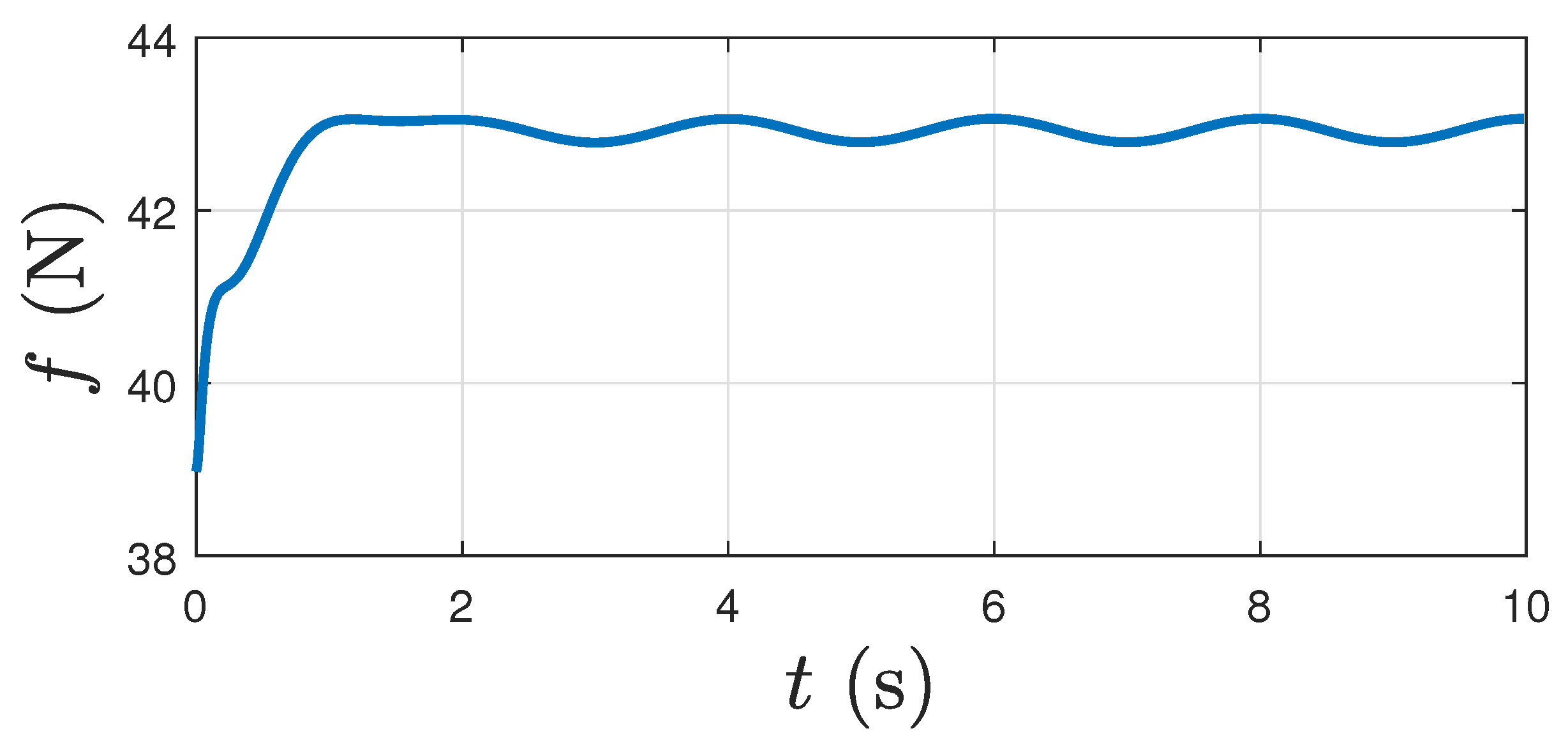
Figure 6 shows the thrust magnitude required to track the desired trajectory, under the influence of disturbance torque. Note that the thrust here is the sum of the four forces generated by rotors of the quadcopter. Each of these forces vary with time and affect the dynamics of the vehicle according to the Equation (44) in [
44], which is omitted here for brevity.
Figure 7 shows components of the angular velocity tracking error,
, and how within 3 seconds they converge to a small neighborhood of the zero vector such that
rad/s, under the influence of disturbance torque. The magnitude of the attitude tracking error is given by the principal angle
of the attitude tracking error
Q.
is obtained from the following expression:
Figure 8 shows the time profile of
under the influence of the disturbance torque.
Figure 9 shows the magnitude of the proposed control torque over time under the influence of the disturbance torque.
5.3. Effectiveness of the Geometric Integral Term
The effectiveness of the geometric integral term in the proposed integral geometric attitude control is shown by the following comparison. Under the existence of disturbance torque, we first use the geometric PD-type attitude controller of [
44] followed by our proposed attitude controller to track the same trajectory, and compare the results.
Figure 10 shows that for the PD-type controller, components of
do not converge to zero but oscillate with noticeable amplitudes about it. On comparing this figure with
Figure 7, we see that the proposed controller shows significantly better performance.
Figure 11 shows rapid oscillations in control that will likely not be realizable by, and therefore should not be implemented on, a quadrotor UAV. Comparing
Figure 9 with
Figure 11, the proposed controller shows remarkably better performance with negligible oscillations. In addition,
Figure 11 shows the large magnitude of the required control torque given by the geometric PD-type controller. Note that much less control effort is needed by the proposed controller (
Figure 9), compared to the geometric PD-type controller (
Figure 11), to track the same trajectory.
Figure 12 shows the norm of the attitude tracking error (given by the principal angle of the rotation matrix
Q) for both PD and the proposed controllers. The proposed controller shows this error to decrease more smoothly and with less oscillations than the PD-type controller.
Overall, the comparison in this subsection shows that the proposed controller has significant advantages over a PD-type controller in steady-state performance as well as disturbance attenuation. It tracks the same maneuvering attitude trajectory better while requiring significantly less overall control effort under the influence of a time-varying disturbance torque.
5.4. Comparisons in the Zero Disturbance Case
Here, we make observations based on numerical simulations comparing the performance of the proposed controller under influence of disturbance that was presented in
Section 5.2, with its performance when there is no disturbance (
) while tracking the same desired trajectory. If the disturbance is zero, then the proposed controller gives the following results in numerical simulation.
Figure 13 shows components of the angular velocity tracking errors over time, which converge asymptotically to zero. This case (
) can be thought of as an ideal case, and by comparing
Figure 7 with the above figure, we see there is little change in the performance of the proposed controller under the influence of a disturbance. The time plots in
Figure 7 show a similar tracking profile to the ideal case of zero disturbance (
Figure 13).
Figure 14 shows the control torque magnitude, as given by the proposed controller when there is no disturbance, i.e.,
. Again, considering this case as an ideal case, we see that the proposed controller performs robustly in the presence of disturbance. The profile in
Figure 9 is similar (with minor oscillations) to that of
Figure 14. The following zoomed-in
Figure 15 shows that when the disturbance torque acts, components of
converge to, and remain in, a small neighborhood of the zero vector, which is the expected result from Theorem 2. In addition, note that when there is no disturbance, components of
converge to zero, as shown in
Figure 16.
To summarize, in this section we compared the performance of the proposed integral geometric attitude tracking controller for two situations, one when there is no disturbance torque (ideal case) and the other when a disturbance torque acts. We observed that under the influence of a disturbance torque the proposed controller performs well, and results in similar but slightly degraded performance, compared to the ideal case of zero disturbance.


