Article

Bi-Level Fuzzy Expectation-Based Dynamic Anti-Missile Weapon Target Allocation in Rolling Horizons

Air Defense and Anti-Missile College, Air Force Engineering University, Xi’an 710051, China
*
Author to whom correspondence should be addressed.
Electronics 2022, 11(19), 3035; https://doi.org/10.3390/electronics11193035
Submission received: 1 August 2022 / Revised: 19 September 2022 / Accepted: 20 September 2022 / Published: 23 September 2022
(This article belongs to the Section Systems & Control Engineering)

Abstract

:
The weapon target allocation (WTA) problem is a crucial issue in anti-missile command decisions. However, the current anti-missile weapon target allocation models ignore the dynamic complexity, cooperation, and uncertainty in the actual combat process, which results in the misclassification and omission of targets. Therefore, we propose a bi-level dynamic anti-missile weapon target allocation model based on rolling horizon optimization and marginal benefit reprogramming to achieve rapid impact on static and dynamic uncertainties in the battlefield environment. Further, we also propose an improved bi-level recursive BBO algorithm based on hybrid migration and variation to perform fast and efficient optimization of the model objective function. A simulation analysis demonstrate that the model is suitable for larger-scale, complex, dynamic anti-missile operations in uncertain environments, while the algorithm achieves better solution efficiency and solution time compared with the same type of heuristic algorithm, which meet the requirements of solution accuracy and timeliness. In addition, we obtain better rolling horizon parameters to further optimize its performance.

1. Introduction

With the advent of the information warfare era, battlefield information is transferred and exchanged among multiple weapon platforms. As a result, anti-missile allocation is subjected to disruption by various factors, such as enemy electronic interference and cyber attacks, as well as environmental noise and the limitations of combat platforms. Ultimately, the acquisition of battlefield information is constrained. In these circumstances, it is impossible to achieve an operational objective all at once, which requires full consideration of target allocation, scheduling, and synergy effectiveness. Therefore, a dynamic anti-missile weapon target allocation problem is modeled in this paper considering the above operational characteristics.
There are two key components in carrying out dynamic weapon target allocation: the weapon target allocation (WTA) problem and the firepower-scheduling problem (FSP). In addition, it is necessary to carefully consider the cooperative effects of different weapon platforms, which is significant to achieving a synergistic effect among multiple combat units and maximizing the overall effectiveness. In this paper, a weapon is taken as a weapon platform for anti-missile warfare, a firepower is considered as an interceptor, and a target is treated as an incoming enemy missile target.
In the following section, a brief review is conducted on relevant studies to modeling construction and algorithm solving in the context of WTA and FSP.
First introduced into the combat field by Manne [1], weapon target allocation (WTA) is purposed to maximize combat utility by effectively allocating weapons to targets with the probability of killing considered. With the diversification of combat forms and the expansion of combat scale, the WTA problem has been further studied to solve the original problem from more different perspectives, mainly including static weapon target allocation (SWTA) and dynamic weapon target allocation (DWTA). Classical SWTA models include (1) asset-based SWTA [2]; (2) sensor-based SWTA [3]; (3) effects-based SWTA [4]; (4) constraint-based SWTA [5]; (5) multitarget SWTA [6]; and (6) constrained multitarget SWTA [7]. Since SWTA performs poorly in adapting to the needs of an ever-changing battlefield, DWTA was subsequently proposed. With time as a dimension, DWTA takes into account the state of a weapon target at different times and then performs multiple dynamic and continuous optimization analyses based on SWTA. Classical DWTA models include a DWTA with “time window” optimization, as proposed by Khosla [8]; a Markov decision process model WTA established by Davis et al. [9], who proposed an approximate dynamic-planning method to solve the problem; and a DWTA constructed by Fan [10] for fuzzy chance-constrained two-level planning. The above analysis shows that DWTA has been developed mainly based on two-phase models and “shoot-observe-shoot” models. However, all of these depend on static data of the current phase and the prediction of future phase for offline distribution, which is not as significant to the dynamic analysis of the battlefield.
Currently, there are still few studies on FSP. Ojeong Kwon [11] analyzed the problem of how to adjust a firing sequence for a minimum time span in the field artillery domain, i.e., the fire-scheduling problem (FSP). Young-Ho Cha [12] paid attention to firepower scheduling that minimized the total threat to the target or an adversary that survived the firing attack for single-weapon targets, as well as for multiweapon targets. However, it was easy to find out that the above scheduling minimized the time taken to complete the shot and the threat to the incoming target but ignored resource consumption. Therefore, the high cost of interceptor resources must be carefully considered in the target allocation and scheduling process.
In addition, it is necessary to consider the uncertainties of a battlefield and the impact of synergistic effectiveness between different weapons in anti-missile fire synergy. The commonly used approaches for the quantitative analysis of uncertainties in the anti-missile weapon target problem include the interval gray number [13], fuzzy multi-objective-planning model [14], variable fuzzy clustering preference theory system [15], game model [16], robust model [17], and CvaR conditional value-at-risk model [18]. In addition, fuzzy systems are an effective way to deal with uncertainties [19]. However, most of the above-mentioned models can only deal with one or two static uncertainties in the battlefield, which requires more consideration given to the effects of multiple uncertainties. In addition, the common weapon target allocation models pay less attention to the impact from the synergistic effectiveness of weapon platforms.
In terms of model solving, since the dynamic weapon target allocation in the anti-missile field is NP-complete, heuristic algorithms are highly adaptive and more capable of obtaining near-optimal solutions. Currently, the commonly used heuristic algorithms include genetic algorithms (GAs) [20], bee colony algorithms (ABCs) [21], particle swarm algorithms (PSOs) [22], and more. In addition, some hybrid algorithms based on combinations of exact and heuristic algorithms have also been proposed to address the anti-missile problem. Feng [23] proposed an improved quantum-immune cloning multi-objective optimization algorithm. Chu [24] put forward an LAMGC algorithm characterized by forward-looking marginal greedy construction. Wu [25] adopted a stochastic neighborhood variation strategy to optimize the difference variation algorithm. Xin [26] combined Monte Carlo simulations and proposed a constructive heuristic algorithm based on the concept of marginal back-off to solve the target-sensor-weapon allocation problem based on marginal gains. This method facilitated quick adjustments to the solution. Our paper further presents the concept of marginal benefit, which effectively measures the benefit ratio from marginal firepower and, thus, allows for rapid adjustment to dynamic uncertainty factors. Moreover, there is still much space to improve the efficiency and accuracy of solutions for heuristic algorithms.
First proposed by Simon in 2008, the biogeography-based optimization (BBO) algorithm [27] is a heuristic algorithm that has been demonstrated as superior to most heuristics because of its capability to enhance the exchange and sharing of information through migration rate and the efficiency and accuracy of solution. Proposed by Rifai AP [28] on the basis of the BBO algorithm combined with non-dominated ranking, the NSBBO algorithm is significantly advantageous in scheduling multi-objective problems. However, the model is also disadvantaged by such issues as the single form of migration and variation, as well as a long solution time, which requires further improvement.
Based on the above literature review, this study is aimed to effectively solve the anti-missile weapon target problem, as well as its dynamic complexity, cooperativity, and uncertainty from the following perspectives.
  • An analysis of uncertainty factors is performed. The disruptions caused by multiple uncertainties, such as combat environment, interference from enemy targets, and limited detection equipment, affect the final results of weapon target allocation to varying extents. In this paper, the following uncertainties are mainly considered: the uncertainty of target-type identification results and the destruction probabilities of our weapons are taken as fuzzy variables. Then, the fuzzy expectation model is adopted to construct an uncertainty model, and the reprogramming strategy of marginal benefits is used to solve dynamic uncertainties, such as the emergence of new targets and the disappearance of old targets.
  • A bi-level dynamic weapon target allocation model is proposed. We propose a bi-level dynamic weapon target allocation model in this paper under a rolling horizon framework. For the upper-level objectives, the weapon target allocation problem (WTA) is considered on the basis of synergistic effectiveness, while for the lower-level objectives, the firepower-scheduling problem (FSP) is considered. This reflects the coupling and constraint relationships between multiple combat targets, which makes the model more closely related to combat needs.
  • An improved bi-level recursive BBO algorithm is proposed on the basis of hybrid migration and variation for solving the model. Given a certain degree of complexity of the bi-level model, it is necessary to develop new intelligent algorithms for the corresponding solution. In this paper, the BBO algorithm is adapted for the multi-objective bi-level programming model. In addition, an improved BBO algorithm is proposed separately to solve the multi-objective bi-level programming model in an efficient way.

2. Problem and Model

In this section, we firstly analyze the uncertainty factors for anti-missile operations; secondly, we introduce the optimization strategy of rolling horizon; and finally, we propose a bi-level dynamic weapon target allocation model.

2.1. Uncertainty Factor Analysis

Anti-missile warfare is an information game process under uncertain conditions, and most of the existing anti-missile weapon target allocation model are deterministic models, which seldom consider the influence of uncertainties in warfare. Due to the complexity of the actual battlefield environment and the existence of uncertainties, such as sensor errors and interference effects on tracking and detection equipment, the models and parameters constructed in decision making often have uncertainty characteristics. For the characteristics of static and dynamic uncertainties, we performed the analysis shown in Figure 1, categorized as follows:
  • Static uncertainty: This type of uncertainty does not vary with time, which can be caused by the limitations of the sensor detection capability and the penetration characteristics of incoming targets so that the measured data and the acquired battlefield information are uncertain, and the degree of uncertainty is difficult to measure.
  • Since this uncertainty is characterized by ambiguity and mainly affects the relevant parameters in the model, the following two static uncertainties were considered.
    (1)
    Target threat degree: The target threat degree is affected by kinematic information, such as the speed and altitude of missiles, and is related to the degree of real-time and the accuracy of information obtained. If a target has a higher threat level to our target, priority is given to shoot it in order to obtain a greater effect of destruction and protection of our assets. The target threat level under information-based conditions requires not only state information, such as the target’s speed, altitude, and heading angle, but also tactical information, such as target type, maneuver behavior, and game strategy, and thus has a strong uncertainty characteristic.
    (2)
    Damage probability: Due to the high cost of weapons and equipment, the probability of destruction can only be derived from simulation and historical data, which has obvious uncertainty characteristics in the complex anti-missile environment.
2.
Dynamic uncertainties: Dynamic uncertainties change with time, and their changes often have a great impact on the overall anti-missile process model by changing the characteristic and structure, such as the type and model of the targets, the trajectory of the motion state, the results of true and false identification, the sudden change in the target information, etc. The time and scale of their occurrence are unknown relative to the decision-making moments. In this paper, we considered two cases of dynamic uncertainties, i.e., the emergence of new targets and the disappearance of old targets.
In this paper, the target threat degree and damage probability were depicted as fuzzy variables and represented by triangular fuzzy variables. In order to avoid blind consumption and destruction, we established the fuzzy expectation objective function F1. For the dynamic uncertainties generated in this case, we applied a rescheduling strategy to respond to dynamic events in a timely manner when dynamic uncertainties that reached the trigger conditions were generated, and rescheduling was performed based on the original allocation scheduling scheme.
To approximate a battlefield situation, the additional assumptions were made as follows:
  • The enemy maneuvering situation was not considered.
  • The time consumption of wave transfer and ammunition replenishment was not considered.
  • We assumed that the target ballistic prediction and the predicted target time window were accurate enough.
  • Each incoming target was assigned at least one firepower.
  • Each weapon was equipped with multiple firepowers, with a maximum of one fire at a time against each target, and the total number of fires assigned could not exceed the limit on the number of fires for that weapon.
  • A target was considered to be successfully intercepted when the cumulative probability of firepower damage to the target reached the lower limit of severe damage.
  • There were several different interception strategies for intercepting incoming targets, including firing a single interceptor; firing multiple interceptors in unison; “shoot-observe-shoot” and other various strategies; and a combination of different interception strategies.
In order to save firepower and avoid missed interceptions, the “shoot-observe-shoot” strategy was considered in this paper [29].

2.2. Bi-Level Dynamic Weapon Target Allocation Model Construction

The symbols of the parameters used in this paper are shown in Table 1.

2.2.1. Rolling Horizon Optimization Strategy

The idea of rolling horizon optimization could decompose the global optimization problem into subproblems according to the time domain. The application of the rolling horizon strategy helped reduce the complexity of the counter-guided dynamic weapon target allocation problem, which is a large-scale, complex NP problem considering time scheduling.
This strategy could divide the whole generation process of the anti-missile weapon target allocation solution into several local decision processes according to time domain and, finally, form a global decision solution.
Definition 1.
Local decision scheme. The scheduling decision matrix T X ( s ) and the allocation decision matrix D X ( s ) formed in rolling horizon s constitute the local decision scheme.
Definition 2.
Global decision scheme. The scheduling decision matrix T X ( s ) and the allocation decision matrix D X ( s ) of rolling horizon s correspond to form the scheme ( D X ( s ) , T X ( s ) ) , and the final global decision scheme J X = { ( D X ( 1 ) , T X ( 1 ) ) , ( D X ( 2 ) , T X ( 2 ) ) , , ( D X ( s ) , T X ( s ) } is formed in succession according to the sequence of the time domain.
The rolling horizon optimization strategy proposed in this paper used the number of assigned and scheduled targets as the basis for dividing the time domain cycles rather than intervals in time. In this optimization process, the solution obtained in each time domain was used as the input of the next time domain so that the objectives in each time domain could be solved optimally. Each rolling task window could generate one local decision solution, and eventually, multiple local decision solutions formed the global decision solution.
The steps of rolling time domain optimization were as follows.
Step1: Target initialization. Sort the targets according to the earliest interceptable window time and select the top W into the rolling task window.
Step2: Take the W targets entering the task window as input, run the upper-level weapon target allocation algorithm, and keep the top K elite solutions after iterative loop merit search.
Step3: Take the first K elite solutions as input, run the lower-level firepower scheduling algorithm, and obtain the final optimized scheduling result by iterative merit seeking.
Step4: At the end of a rolling task window, evaluate the targets that have been assigned and scheduled, and update the set of decision variables. If the constraint is satisfied, i.e., the maximum probability of destruction is reached, the target is considered to be destroyed, and the allocation and scheduling results of the target are frozen and added to the frozen task sequence; if the constraint is not satisfied, the target enters the next rolling horizon, and so on. Roll forward until all targets are scheduled and assigned, and the constraints are met. Then, the rolling horizon ends.
The specific process is shown in Figure 2. In scenario1, if the constraints are met, freeze the completed target. In scenario2, if the constraint conditions are not met, the target that does not meet the conditions enters the next rolling window and, at the same time, freeze the target conforming to the constraints, and make the target not conforming to the constraints continue to enter the next rolling window for allocation and scheduling, assuming that the target at the current position 3 is not conforming to the constraint (the red target is the target not conforming to the constraint condition, and the red window represents the frozen window).

2.2.2. Upper-Level Multi-Objective Weapon Target Allocation Function

  • Objective function F1:
max F 1 ( d x , t x ) = max E ( N ( d x , t x ) ) min G ( d x , t x )
The objective function is based on the traditional WTA model [30], and the objective is to maximize the expected damage probability and minimize the interceptor consumption. The fuzzy damage probability matrix P ˜ = [ p ˜ i j ] m × n and fuzzy target threat degree vector V ˜ = [ v ˜ 1 , v ˜ 2 , v ˜ j ] are designed to establish the following fuzzy expectation value objective function to maximize the cost efficiency ratio.
max E ( N ( d x , t x ) ) = j = 1 n v ˜ j ( 1 s = 1 r i = 1 m ( 1 p ˜ i j ( t x i j s ) ) d x i j s )
min G ( d x , t x ) = s = 1 T j = 1 n i = 1 m d x i j
where max E ( N ( d x , t x ) ) is to maximize the expected damage probability, and min G ( d x , t x ) is to minimize the interceptor consumption.
2.
Objective function F2:
We considered both the vertical master–slave collaboration between the upper command and decision layer and the lower fire interdiction implementation layer, as well as the horizontal autonomous collaboration relationships between different weapons in the firepower interdiction implementation layer. In order to achieve the above objectives and to make the functions between different weapons complement each other to achieve the goal of maximizing the collaboration effect, the following three aspects of collaboration effect indicators needed to be considered.
Definition 3.
Firepower collaboration effectiveness indicators. This indicator needed to take into account the uniformity of weapon target allocation; that is, for a specific fire weapon, it needed to be allocated to as many targets as possible, thus avoiding the concentration of a few weapons and reducing the overall efficiency. In addition, it needed to consider the consistency of weapon target allocation; that is, the firepower of the same weapon needed to be allocated to the same target as much as possible in permitting conditions.
Definition 4.
Information collaboration effectiveness indicators. The level of information interaction between different weapons affected the realization of collaboration.
Definition 5.
Command capability collaboration effectiveness indicators. We considered the collaborative capability of the operational command and decision layer for the firepower interdiction implementation layer, and this indicator was related to the collaborative command capability.
max F 2 ( d x , t x ) = ω 1 I 1 + ω 2 I 2 + ω 3 I 3
I 1 = m 1 ( j = 1 n | s = 1 r i = 1 m d x i j m n s u m | ) m 2 ( i = 1 m | s = 1 r j = 1 n d x i j m n s u m | ) · s = 1 r i = 1 m j = 1 n d x i j · b i j
I 2 = s = 1 r i = 1 m j = 1 n d x i j · z i j
I 3 = s = 1 r i = 1 m j = 1 n d x i j · o i j
where I 1 is firepower collaboration effectiveness; I 2 is information collaboration effectiveness; I 3 is command capability collaboration effectiveness; b i j is the basic firepower collaboration effectiveness matrix; z i j is the information collaboration effectiveness matrix; o i j is the command collaboration effectiveness matrix generated by expert assessment scoring; ω 1 , ω 2 , ω 3 are weighting coefficients; m 1 , m 2 are scaling factors, which should be determined according to actual battlefield conditions; and n s u m m is the sum of the incoming targets in all rolling horizons.
3.
The constraints:
s . t . s = 1 r j = 1 n x i j C i
1 s = 1 r i = 1 m ( 1 p ˜ i j ( t x i j s ) ) d x i j s ) D max
i = 1 m d x i j 1
s = 1 r j = 1 n i = 1 m d x i j i m C i
where Equation (8) indicates that the total number of firepower allocated to targets did not exceed the maximum number of firepower for that weapon. Equation (9) indicates that the cumulative probability of killing each target needed to reach or exceed the severe destruction boundary value D max for that target (then the target was considered destroyed). Equation (10) indicates that, in rolling horizon s, each target was assigned at least one firepower. Equation (11) indicates that the total number of firepower allocated could not exceed the sum of the number of firepower of all the weapons.

2.2.3. Lower-Level Firepower Collaborative Scheduling Function

For each interceptable target, in its ballistic trajectory prediction, an earliest predicted interception point and a latest predicted interception point could be obtained, thus forming an interceptable time window, where t j e s t is the earliest interceptable moment and t j l s t is the latest interceptable moment. Since earlier (later) than the earliest (latest) interceptable moment leads to the missed interception of a target, to meet the purpose of avoiding missed interception and early coordinated interception, the following objective function could be set.
min F 3 ( d x , t x ) = min ( s = 1 r j = 1 n ( μ max ( 0 , t j e s t t x i j s ) + β max ( 0 , t x i j s t j l s t ) ) + max i M , j N { t x i j s } )
s . t . t x q s t x j s + S W j q σ j q + D W j q ( 1 σ j q ) ϑ z q j
where ( j , q ) is a pair of targets scheduled in pre-post order, j , q N ; σ j q indicates whether target j and target q are assigned to the same weapon if σ j q = 1, otherwise σ j q = 0; σ q j + σ j q = 1 ; and z j q is whether target j intercepts and dispatches before target q if z j q = 1, otherwise, z j q = 0; z j q + z q j = 1 .
In Equation (12), μ   β , are set as the penalty factors, which are large positive integers, and the penalty is applied when the scheduling moment t x i j s of target j exceeds its time window ( t j _ e s t , t j _ l s t ) . max i M , j N { t x i j s } indicates that the moment of the latest target to be intercepted among the current targets to be scheduled is selected, and minimizing the max i M , j N { t x i j s } achieves target interception as early as possible.
In Equation (13), we considered the single flak firepower channel occupancy time and ballistic crossover problem. When σ j q = 1, the firepower channel occupancy time before and after the flak is S W j q ; when σ j q = 0, the time interval D W j q between firepowers of different weapons needs to be satisfied so that no ballistic crossover occurs during the flight of the interceptor. ϑ is a penalty factor, and the inequality holds only when z q j = 0, i.e., when target q intercepts before target j do not hold.
The schematic diagram of the bi-level model is shown in Figure 3. The left side of the image shows the overall global decision process for the weapon target allocation, and the right side shows the local decision process in one of the rolling horizons. The upper level in the local decision makes weapon target allocation and outputs the solution to the lower level, and then the lower level makes fire dispatch and outputs the solution to the upper level for feedback correction to obtain the final local decision solution. Finally, the local decision solution returns to the global process on the left side to form the global decision solution.

2.2.4. Reprogramming Strategy Based on Marginal Benefits

When dynamic uncertainties occurred, elements in the weapon–target set of the solutions for weapon target allocation changed, and the solution needed to be adjusted in time to accommodate the requirements of the sudden change uncertainties. Dynamic un-certainties, which included the emergence of new targets and the disappearance of old targets, could be discussed as follows.
When new targets appeared, the existing weapon–target allocation scheme corresponded to the original set of observed weapons and targets, and the new targets needed to be inserted into the appropriate rolling window, and the target assignment scheme already generated in that rolling window needed to be adjusted for reprogramming, which included weapon–target reallocation and fire rescheduling. There were two main types of cases when old targets disappeared. The first type was that, after a flush fire, the firepower achieved a heavy damage effect on the target, and then the target was considered destroyed and entered the frozen window. The second type was that, after a flush fire, the firepower did not achieve a heavy damage effect on the target, and then the target needed to enter the next rolling window, and the weapon and target collection was updated accordingly.
There were differences in the timing of reallocation and rescheduling solutions under the above two uncertainties. For the disappearance of old targets, the cases that needed to be considered for reallocation and rescheduling were mainly in the second category, which required the reallocation and rescheduling modification of solutions already generated in the next rolling time domain; for the emergence of new targets, it was necessary to determine whether the currently existing weapon–target allocation and firepower-scheduling solutions reached the maximum output moment, i.e., the time when the weapon was to fire according to the solution. If it was reached, the existing solution was output, and the new target was included in the new rolling window, with an operation procedure that was the same as the disappearance of the second type of old targets; if it was not reached, the reprogramming strategy was executed.
For each old and new target to be reallocated and rescheduled, we applied the concept of marginal benefit, i.e., firepower was allocated to any one target based on the original weapon–target solutions so that the increment of the probability of expected damage probability Δ E ( N ( d x , t x ) ) , the increment of the collaboration effect Δ F 2 ( d x , t x ) , and the negative increment of interceptor consumption Δ G ( d x , t x ) could be obtained for that firepower. The increment of expected destruction probability Δ E ( N ( d x , t x ) ) and the increment of collaboration effect Δ F 2 ( d x , t x ) could be used as the increment of change in benefit to measure the marginal benefit of weapon allocation and firepower scheduling. The negative increment of interceptor consumption Δ G ( d x , t x ) could be used as the increment of change in cost to measure the marginal benefit of firepower allocation and scheduling, thus obtaining the formula for the marginal benefit of interceptor allocation.
M e ( d x , t x ) i j = α ( Δ E ( N ( d x , t x ) ) + Δ F 2 ( d x , t x ) ) β Δ G ( d x , t x )
where α and β are weight coefficients, which satisfy the equation α + β = 1   ( 0 α 1 ,   0 β 1 ) , to measure the decision maker’s degree of preference among the increment of expected damage probability, the increment of collaborative effect, and the increment of interceptor consumption.
The specific steps were as follows:
Step1: Initialize the set of weapons and targets in the current rolling window. Let the set of weapons that is already assigned be M , the set of targets that is already assigned be N , and the set of new targets to be reassigned be N . We assumed that the probability of destruction of different firepower in any weapon for a particular target was the same.
Step2: Calculate the marginal benefit brought by one weapon allocated to each target set N in the set M , obtaining the set of marginal benefits { M e ( d x , t x ) i j } .
Step3: Select a target with minimal marginal benefits (for the case where there are multiple weapons assigned to the same target j, the largest { M e ( d x , t x ) i j } among them is selected for comparison). According to Step2, replace the new target in the set N , forming the new target set as N n e w . According to the marginal benefit of the initialize set M and N , the superior weapons are selected, reallocated, and rescheduled with priority.
Step4: Obtain the new reallocation and rescheduling scheme.
The flow chart of the reallocation and rescheduling strategy is shown in Figure 4.

3. Improved Bi-Level Recursive BBO Algorithm Based on Hybrid Migration and Variation

The biogeographic optimization algorithm simulates a migration model of species in nature. The solution of the algorithm is described as “Habitat”, and habitats that are considered suitable for species have a high habitat suitability index (HSI), with factors related to this index described as suitability index variables (SIVs). A SIV can be considered as the independent variable of a habitat, and the HSI can be considered as the dependent variable. The algorithm achieves solution diversity through migration and variation operations. Compared with other optimization algorithms, the BBO algorithm has some obvious advantages: in a BBO, the original population does not disappear after each generation but is modified by migration, and its attributes are shared directly between different solution solutions, thus allowing a better information flow; at the same time, the BBO algorithm has good mining ability and global search ability for candidate solutions, and the retention mechanism for elite solutions allows good solutions to be preserved and not modified in the iterations. These advantages are superior for solving NP-hard problems.

3.1. Upper-Level INSBBO Algorithm

The upper problem objective function was a multi-objective optimization problem (MOP), and an NSBBO algorithm is an intelligent algorithm based on the BBO algorithm after combination with a non-dominated sorting method, which extends from solving single-objective problems to solving MOPs and was proved by the original authors for its speed and accuracy in solving. However, there are still some problems in this algorithm: there is poor ability to explore solution diversity and the migration method is relatively single and time-consuming. For solving this problem, the hybrid migrator and variational operator proposed were improved adaptively in this paper, and the improvement process was as follows.

3.1.1. Upper-Level Algorithm Coding

Bi-level coding was used, where the upper level was coded for the specific firepower allocation of weapons, and the lower level was coded for the correspondence between firepower and targets. The specific process is shown in Figure 5 if there are two weapons, W1 and W2, each equipped with a firepower quantity of two, and three incoming targets, T1, T2, andT3. Each element in the first level of coding was randomly assigned a value of 0 (or 1), indicating whether the firepower of weapon i was assigned to the corresponding target; the elements in the second-level code were randomly assigned values of { 1 , 2 , 3 } to indicate which firepower was assigned to the corresponding target.

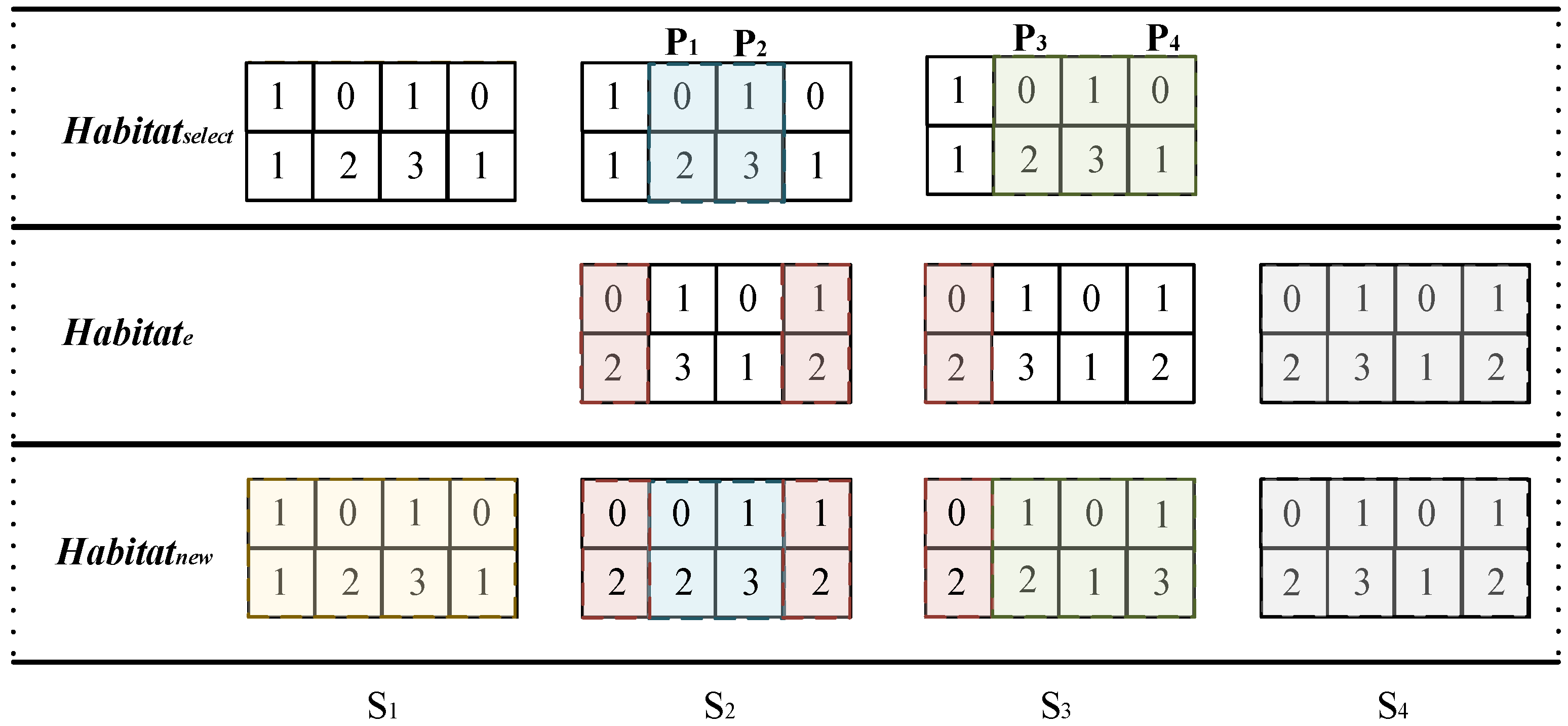
3.1.2. Hybrid Migration Operator

As the migration operator in NSBBO is relatively single and complex to operate, this paper proposed several new migration operators to form a hybrid migration operator whose operation process is reflected in Figure 6, and the specific operation process was as follows.
Step1: Supposing there are popsize habitats (solution scheme) and the current habitat is Habitate, the Habitatselect is randomly selected from all habitats by roulette; then, the migration operation is completed by the hybrid operator formed by the four migration operators S1, S2, S3, and S4.
Step2: The migration condition in the S1 case is with random probability r a n d [ 0 , 0.25 ) . The migration method is to directly copy the Habitatselect selected by roulette to form Habitatnew.
Step3: The migration condition in case S2 is with random probability r a n d [ 0.25 , 0.5 ) . The migration method is to generate position P1 and position P2 in the encoding by random probability and to form Habitatnew by combining the encoding parts of position 1 to position P1 and position p2 to position 4 in Habitate, as well as the encoding part of position P1 to position P2 in Habitatselect..
Step4: The migration condition in case S2 is with random probability r a n d [ 0.5 , 0.75 ) . The migration method is to generate encoded position P3 and position P4 in the encoding by random probability, and the encoded parts from position 1 to position P2 in Habitatselect are migrated to the same positions in Habitatnew in reverse order; then, the remaining position parts of Habitate are combined to form Habitatnew.
Step5: The migration condition in case of S4 is to keep the current habitat Habitate unchanged with random probability r a n d [ 0.75 , 1 ] .

3.1.3. Hybrid Variation Operator

No specific variation operator is proposed in the NSBBO algorithm, and to increase the diversity of the population, the following hybrid variation operator was proposed in this paper and the process is reflected in Figure 7.
Step1: Assuming that there are popsize habitats (solution scheme) and the current habitat is Habitate, then the migration operation is completed by the mixed variation formed by the four variation operators S1, S2, S3, and S4.
Step2: The variation condition in S1 case is when the random probability is r a n d [ 0 , 0.25 ) . Position P1 and position P2 are in the encoding by random probability, while the encoding of the P1 and P2 positions are exchanged to form Habitatnew.
Step3: The variation condition in S2 case is when the random probability is r a n d [ 0.25 , 0.5 ) . Habitatnew is formed by regenerating the encoding parts of P1 and P2 by generating position P3 and position P4 in the encoding with random probability.
Step4: The variation condition in S3 case is when the random probability is r a n d [ 0.5 , 0.75 ) . The encoding of each position is mutated to the encoding of the previous position to form Habitatnew.
Step5: The variation condition in S3 case is when the random probability is r a n d [ 0.75 , 1 ] . The position P5 in the encoding is randomly inserted into the other positions by random probability to form Habitatnew.

3.1.4. Hybrid Variation Operator

Since the NSBBO algorithm is prone to the situation when the objective function value F1 of one solution scheme is smaller than the other objective function value F1 in the operation process, if their objective function values of 2 were very similar, in order to make the distribution of solution schemes on the same Pareto front surface more uniform, solutions with similar arrangements were deleted.

3.1.5. Mixed Elite Mechanism

A new solution scheme was formed by each iteration, and the top z elite populations were archived. After entering the next iteration, the next z populations in the current iteration in the ranking were replaced with the elite populations.

3.2. Lower IBBO-Solving Algorithm

Since the lower objective function was a time-dependent continuous constrained optimization problem, this paper added the hybrid migration operator and hybrid variational operator mentioned in the INSBBO algorithm to the original BBO algorithm and improved the selection mechanism to enhance the algorithm’s optimization-seeking capability, and it could better meet the timeliness requirement in the simulation example.

3.2.1. Algorithm Coding

This coding level generated the target order mainly by random order and generated the order of weapons randomly for each target. As the left part of Figure 8, the interception order of the targets was randomly generated as T1 and T2; the encoding of position 1 and 2 meant that the targets were intercepted in the order of W1 toW2 against target T1. After the coding was completed, the solution result in the upper algorithm was loaded, as in the right part of Figure 8, and if W2 was not assigned to T1 according to the upper algorithm allocation, the coding correction of position 2 was 0.

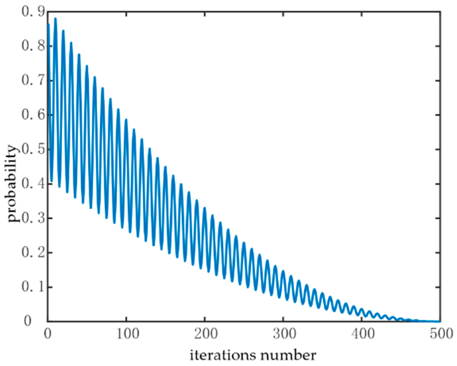
3.2.2. Cosine Adaptive Migration Pressure Selection Mechanism

Based on the original BBO, this paper proposed the following selection probabilities for the migration operator of the original algorithm.
P k = μ k a i p o p s i z e μ i a
a = p d max ( p d max p d min ) ( G G max ) 2
where P k is the probability of the kth solution selected for migration; popsize is the population size; u k is the emigration rate of the habitat; μ i is the immigration rate of any ith habitat; a is the cosine adaptive factor; pdmax is the initial value of the variation in the selected pressure factor; and pdmin is the final value of the variation in the selected pressure factor. Let the initial change probability of pdmax = 1, which gradually decreases to pdmin = 0.1 as the number of generations increases. G is the current number of iterations, Gmax is the maximum number of iterations, and μ i is the selection probability of the current habitat i. Figure 9 reflects the trend in the cosine dynamic adaptive factor a, and the probability of a random probability less than a is larger in the pre-iteration period. The S1, S2 migration operator is mainly beneficial to maintain the diversity of the population and avoid local optimum. At a later stage, the probability of a random probability greater than a is larger, and the S3, S4 migration operator is mainly used for modification, which facilitates more favorable exploration of the solution and is also conducive to the convergence of the algorithm. The cosine dynamic adaptive strategy presented the dynamic change pattern in oscillation, as well as the overall decreasing convergence trend. It avoided the singularity of the modified strategy and facilitated the exploration of the unknown solution, which could avoid the phenomenon of similarity and the duplication of solutions. The trend of cosine factor is shown in Figure 9.
In this paper, a more representative, multi-peak, indistinguishable Ackley test function was selected to run to obtain the results shown in Figure 10, where the red line segment is the unimproved BBO algorithm. It is easy to find that the improved dynamic habitat selection formula converged slowly in the early stage, which was conducive to the global search. It converged quickly in the later stage, which was conducive to strengthening the local search, and it achieved better results and a greater improvement in habitat selection than the original BBO.

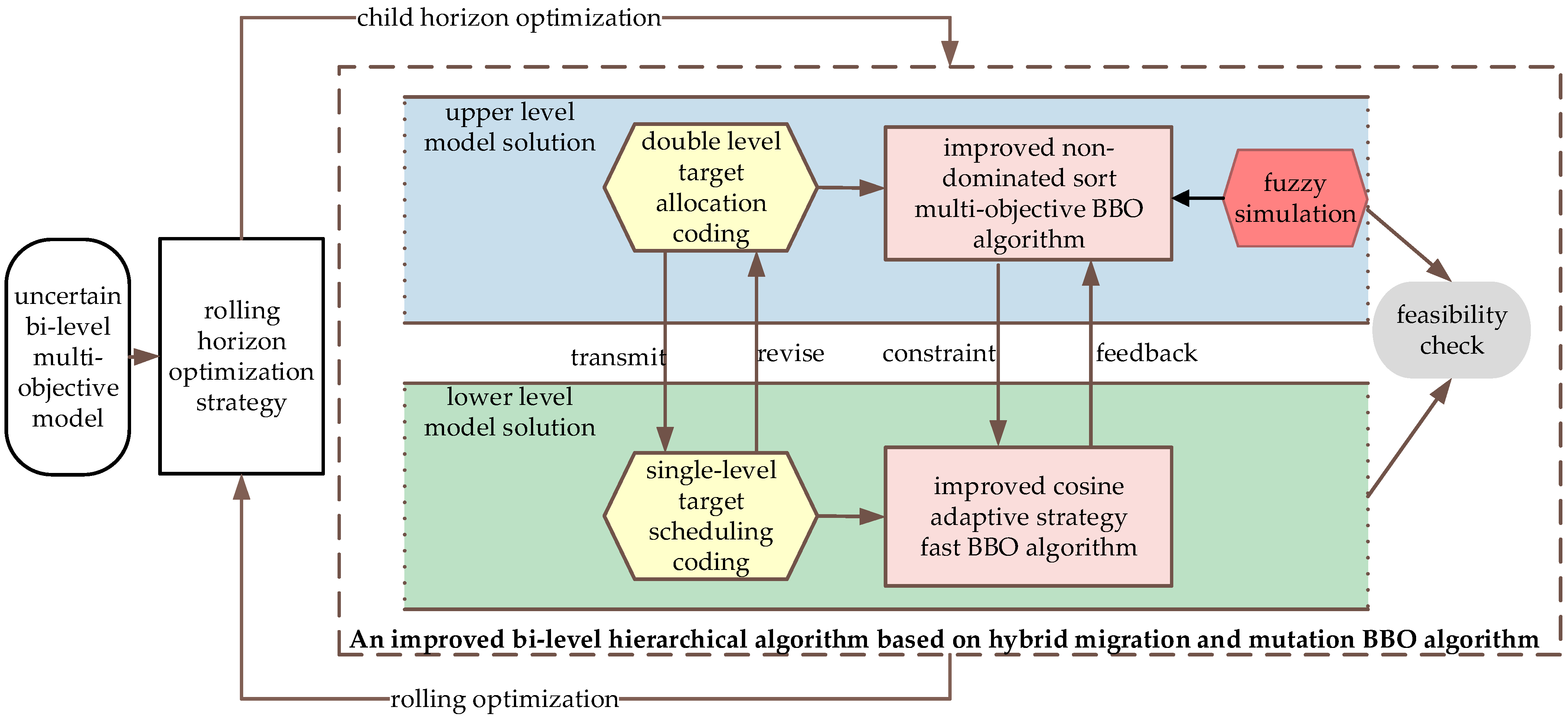
3.3. Improved Bi-Level Recursive BBO Algorithm Based on Hybrid Migration and Variation

The improved NSBBO algorithm for solving the upper model combined with the fuzzy simulation technique [31] and the improved BBO algorithm for solving the lower model were combined with each other to form an improved bi-level recursive BBO algorithm based on hybrid migration and variation, and the specific flow chart of the algorithm is shown in Figure 11.

4. Experiment and Analysis

4.1. Parameter Analysis

4.1.1. Rolling Horizon Window and Anti-Missile Fire Collaboration Problem Scale Study

Tests were conducted for the number of targets W in the task window of the rolling horizon. Since the overall number of targets T varies in problems of different sizes, in order to facilitate a generalizability test for the parameter W, this paper converted the number of W into W e = W / T , where W e denotes the ratio of the number of targets in the task window to the overall number of targets. Since W e was mainly based on the number of targets, the number of weapons was fixed to nine in order to reduce the variables, and each weapon was equipped with 20 firepower. The experiment sizes were small-scale (9 weapons—10 incoming targets); medium-scale (9 weapons—50 incoming targets); and large-scale (9 weapons—100 incoming targets). Each experiment was conducted 10 times individually and averaged.
The parameters were: the same weapon-firing time interval of SW = 0.5 s; the firing time interval between different weapons of DW = 2 s; Dmax = 0.75; ω 1 = 0.4 ;   ω 2 = 0.3 ;   ω 3 = 0.3 ;   α = 0.5 ;   β = 0.5 ; m 1 = 0.5 ; and m 2 = 0.5 . The algorithm parameters were set as follows: number of populations = 50; upper coding dimension = 260; lower coding dimension = 9; maximum variation probability = 0.05; maximum migration modification rate = 0.85; maximum number of iterations = 200; pdmax = 1; and pdmin = 0. Other relevant data were generated from anti-missile combat simulations.
From the Figure 12 analysis, too-small W e values led to repeated calculations and the problem of “short-sightedness”, resulting in a large computational burden, high time cost, and poor solution quality, while too-large W e values had obvious shortcomings in solving small-scale problems. The above experimental results conclude that the determination of W e needed to be determined according to different operational objectives, and a larger W e value could be chosen to enhance the quality of the solution in a case of sufficient time. In a case of time constraint, a smaller W e value was chosen to increase the solution speed; meanwhile, it was necessary to avoid choosing too-small or too-large W e values, which could neither increase the quality of the solution nor reduce the burden of the solution time.

4.1.2. Study on the Length and Distribution of Interceptable Time Window

Each target had an interceptable time window, and the length and distribution of the interceptable time window affected the results of the dynamic weapon target allocation. This paper explored the impact of different lengths and distributions of interceptable time windows on the allocation and scheduling results by designing them. The impact on the target interceptable time window is discussed as follows.
The distribution of interceptable time windows was mainly discussed in three types: (1) the type with concentrated distribution, i.e., the interceptable time windows completely overlapped; (2) the type with moderate distribution, i.e., the interceptable time windows half overlapped; and (3) the type with dispersed distribution, i.e., the interceptable time windows did not overlap at all. The distribution is shown in Figure 13.
The interceptable time window length was mainly discussed in three types (1) short interceptable time window length, (2) moderate interceptable time window length, and (3) long interceptable time window length.
In this paper, the orthogonal test design method was used to construct a test example for a two-factor, three-level test. The orthogonal table was selected, and the construction examples and specific contents are shown in Table 2. The test parameter environment was: assume there are nine weapons, and each weapon is equipped with 20 fires; there are 30 incoming targets; and, according to the parameter analysis in the previous section, make W = 10. Other parameter settings were the same as in Section 4.1.1.
By analyzing Figure 14, we could see that the function value of F1 was affected by the interceptable time window under different levels of influence: moderate > short > long under the length of interceptable time window; and moderate > scattered > concentrated under the distribution of interceptable time window. The function value of F2 was affected by the interceptable time window: short > moderate > long under the length of interceptable time window; and interceptable time window distribution, moderate > dispersion > concentration. The F3 function values were affected by the interceptable time window: interceptable time window length from longer > moderate > shorter; and interceptable time window distribution from dispersion > moderate > concentration. As the F1 and F2 functions were solved for the maximum value, we could moderate and short interception time window lengths and a moderate interception time window distribution were more suitable for the solution of the upper function; the F3 function was solved for the minimum value, so shorter and concentrated interception time window lengths and distributions were more suitable for the solution of the lower function. In the actual solution process, we needed to analyze according to the actual situation.

4.2. Analysis of Scenes

4.2.1. Simulation Experimental Hypothesis

Supposing there were nine weapons, each equipped with 20 fires, and there were 30 incoming targets, the parameter settings were the same as in Section 4.1.1.

4.2.2. Simulation Experiment Results and Analysis

In Figure 15, we compare the solution algorithm of INSBBO with NSBBO and two classical multi-objective algorithms, NSGA-II and MOPSO; in Figure 16, we compare the IBBO algorithm with BBO and two classical single-objective algorithms, GA and PSO. It is easy to see from the image analysis that the Pareto front surface of the INSBBO algorithm was significantly better than the other comparison algorithms in the multi-objective experiments, and combined with the analysis in Table 3, we can see that the algorithm was only second to the MOPSO algorithm in terms of solution time, but the solution results were due to the MOPSO algorithm.
In the single-objective experiment, the convergence of the optimal values of the four algorithms was relatively close, among which the convergence value of the IBBO algorithm was optimal, and the solution time consumed the least. From this analysis, it can be obtained that the bi-level solution algorithm consisting of the INSBBO and IBBO algorithms had advantages in terms of solution efficiency and effectiveness.
The allocation and scheduling scheme without considering the new target emergence factor is reflected on the left side of Figure 17, where there is a situation in which the old target did not reach the heavy destruction efficiency in the T2 phase, and the minimum marginal benefit target was selected to exit the set by calculating the marginal benefit of the target set in the next time domain, and the old target was made to replace. To consider the target redistribution and scheduling in the case of new target emergence, it was assumed that a new target emerged at t = 410 s, 430 s, and 450 s, respectively, and the new target interceptable time windows were [410, 1050], [430, 1350], and [450, 1450], respectively. A new reprogramming solution was obtained according to the marginal benefit redistribution strategy, as the right side of Figure 17 shows. In the initial allocation scheme generated on the left, the red target in the T2 stage did not reach the maximum destruction efficiency in the observation and needed to enter the next stage for continued allocation and scheduling; in the scheme generated on the right, the green target is the newly emerged target, and the new scheme of reallocation was obtained according to the marginal benefit calculation.

5. Conclusions

In this paper, a bi-level fuzzy expectation model under a rolling horizon strategy was proposed, which effectively solved the dynamic complexity, synergy, and uncertainty characteristics in the dynamic weapon target allocation problem of anti-missile fire. We also proposed an improved bi-level recursive BBO algorithm based on hybrid migration and variation to solve the upper-level objective function and an improved biogeographic optimization algorithm to solve the lower-level objective function. The upper-level optimization algorithm proposed hybrid migration and variation operators, a similar solution deletion mechanism, and a hybrid elite mechanism, and the lower-level optimization algorithm introduced a hybrid migration operator, a hybrid variation operator, and an adaptive strategy. In the simulation example, the algorithm reflected better time efficiency and convergence accuracy and could adapt to the solution of large-scale problems. In the next step, we plan to introduce a fuzzy system for the dynamic planning and control of the weapon target allocation problem.

Author Contributions

Conceptualization, C.F.; methodology, X.Z.; software, X.Z.; validation, X.Z., S.L. and H.X.; formal analysis, X.Z.; investigation, C.Q.; resources, C.F.; data curation, X.Z.; writing—original draft preparation, X.Z.; writing—review and editing, S.L.; visualization, C.F.; supervision, C.F.; project administration, C.F.; funding acquisition, C.F. All authors have read and agreed to the published version of the manuscript.

Funding

This work was supported in part by the National Natural Science Foundation of China under Grant 72001214 and Grant 62106283.

Acknowledgments

The authors greatly appreciate the reviews, valuable suggestions, and editors’ encouragement.

Conflicts of Interest

The authors declare no conflict of interest.

References

  1. Manne, A.S. A target-assignment problem. Oper. Res. 1958, 6, 346–351. [Google Scholar] [CrossRef]
  2. Shang, G.; Zaiyue, Z.; Xiaoru, Z. Immune genetic algorithm for weapon-target assignment problem. Intell. Inf. Technol. Appl. 2007, 7, 145–148. [Google Scholar]
  3. Bogdanowic, Z. A new efficient algorithm for optimal assignment of smart weapons to targets. Comput. Math. Appl. 2009, 58, 1965–1969. [Google Scholar] [CrossRef]
  4. Wang, M.; Fan, Y. Intelligent solving algorithm for effects-based firepower allocation model of conventional missiles. Syst. Eng. Electron. 2017, 39, 2509–2514. [Google Scholar]
  5. Lee, M.Z. Constrained weapon–target assignment: Enhanced very large scale neighborhood search algorithm. IEEE Trans. Syst. Man Cybern. 2010, 40, 198–204. [Google Scholar] [CrossRef]
  6. Volle, K.; Rogers, J. Weapon–target assignment algorithm for simul-taneous and sequenced arrival. J. Guid. Control Dyn. 2018, 41, 2361–2373. [Google Scholar] [CrossRef]
  7. Zhang, K.; Zhou, D.Y.; Yang, Z. Constrained multi-objective weapon target assignment for area targets by efficient evolutionary algorithm. IEEE Access 2019, 7, 176339–176360. [Google Scholar] [CrossRef]
  8. Khosla, D. Hybrid genetic approach for the dynamic programming for missile defense interceptor fire control. Eur. J. Oper. Res. 2016, 242, 1–14. [Google Scholar]
  9. Davis, M.T.; Robbins, M.J.; Lunday, B.J. Approximate dynamic programming for missile defense interceptor fire control. Eur. J. Oper. Res. 2016, 259, 873–886. [Google Scholar] [CrossRef]
  10. Fan, C.L.; Xin, Q.H.; Fu, Q. Modeling and realization of dynamic firepower allocation problem based on fuzzy chance constrained bi-level programming. Syst. Eng. Theory Pract. 2016, 5, 1318–1330. [Google Scholar]
  11. Kwon, O.; Lee, K.; Park, S. Targeting and scheduling problem for field artillery. Comput. Ind. Eng. 1997, 33, 693–702. [Google Scholar] [CrossRef]
  12. Cha, Y.H.; Kim, Y.D. Fire scheduling for planned artillery attack operations under time-dependent destruction probabilities. Omega 2010, 38, 383–392. [Google Scholar] [CrossRef]
  13. Zhao, Y.; Chen, Y.F.; Zhen, Z.Y. Multi-weapon multi-target assignment based on hybrid genetic algorithm in uncertain environment. International. J. Adv. Robot. Syst. 2020, 17, 17–24. [Google Scholar]
  14. Xu, H.; Xing, Q.H.; Wang, W. WTA for air and missile defense based on fuzzy multi-objective programming. Syst. Eng. Electron. 2018, 40, 563–570. [Google Scholar]
  15. Wang, S.Q. Application Study of Variable Fuzzy Fet Multi-Attribute Decision Making Theory on Large-Formation Air Defense Decision Making. Ph.D. Thesis, Dalian University of Technology, Dalian, China, 2011. [Google Scholar]
  16. Pan, Q.; Zhou, D.; Tang, Y. A novel antagonistic weapon-target assignment model considering uncertainty and its solution using decomposition co-Evolution algorithm. IEEE Access 2019, 6, 1–12. [Google Scholar] [CrossRef]
  17. Xu, W.; Chen, C.; Ding, S. A bi-objective dynamic collaborative task assignment under uncertainty using modified MOEA/D with heuristic initialization. Expert Syst. Appl. 2020, 140, 1–24. [Google Scholar] [CrossRef]
  18. Li, J.; Xin, B.; Panos, M. Solving bi-objective uncertain stochastic resource allocation problems by the CVaR-based risk measure and decomposition-based multi-objective evolutionary algorithms. Ann. Oper. Res. 2021, 296, 639–666. [Google Scholar] [CrossRef]
  19. Zhao, T.; Cao, H.; Dian, S. A Self-organized method for a hierarchical fuzzy logic system based on a fuzzy autoencoder. IEEE Trans. Fuzzy Syst. 2022, 1, 1–21. [Google Scholar] [CrossRef]
  20. Wang, W.; Liu, X.L.; Wang, J. Method of area antiaircraft weapon target assignment for the warship formation under informationized conditions. Syst. Eng.-Theory Pract. 2015, 35, 1011–1018. [Google Scholar]
  21. Chang, T.; Kong, D.; Hao, N. Solving the dynamic weapon target assignment problem by an improved artificial bee colony algorithm with heuristic factor initialization. Appl. Soft Comput. 2018, 70, 845–863. [Google Scholar] [CrossRef]
  22. Li, L.; Liu, F.; Long, G. Modified particle swarm optimization for BMDS interceptor resource planning. Appl. Intell. 2016, 44, 471–488. [Google Scholar] [CrossRef]
  23. Feng, C.; Yao, P.; Jing, X.N. Weapon-target assignment based on improved quantum-inspired immune clonal multi-objective optimization algorithm. Comput. Eng. Sci. 2017, 37, 2314–2319. [Google Scholar]
  24. Chu, X.G.; Ma, Z.W.; Chen, X.J. Look-ahead margin-greedy constructive algorithm for the multi-objective optimizationof the weapon target assignment problem. Syst. Eng. Electron. 2019, 41, 2252–2259. [Google Scholar]
  25. Wu, W.H.; Guo, X.F.; Zhou, S.Y. Improved differential evolution algorithm for solving weapon-target assignment problem. Syst. Eng. Electron. 2021, 43, 1012–1021. [Google Scholar]
  26. Xin, B.; Wang, Y.; Chen, J. An efficient marginal-return-based constructive heuristic to solve the sensor-weapon-target assignment problem. IEEE Trans. Syst. Man Cybern. Syst. 2018, 1, 1–12. [Google Scholar] [CrossRef]
  27. Simon, D. Biogeography-based optimization. IEEE Trans. Evol. Comput. 2008, 12, 702–713. [Google Scholar] [CrossRef]
  28. Rifai, A.P.; Nguyen, H.T.; Aoyama, H. Non-dominated sorting biogeography-based optimization for bi-objective reentrant flexible manufacturing system scheduling. Appl. Soft Comput. 2018, 62, 187–202. [Google Scholar] [CrossRef]
  29. Kalyanam, K.; Casbeer, D.; Pachter, M. Monotone optimal threshold feedback policy for sequential weapon target assignment. J. Aerosp. Inf. Syst. 2017, 14, 68–72. [Google Scholar] [CrossRef]
  30. Karasakal, O. Air defense missile-target allocation models for a naval task group. Comput. Oper. Res. 2008, 35, 1759–1770. [Google Scholar] [CrossRef]
  31. Liu, B.; Liu, Y.K. Expected value of fuzzy variable and fuzzy expected value models. IEEE Trans. Fuzzy Syst. 2002, 10, 445–450. [Google Scholar]
Figure 1. Uncertainty factor classification diagram.
Electronics 11 03035 g001
Figure 2. Flowchart of rolling horizon scheduling strategy. * M i in the figure denotes weapon i, and N j denotes incoming target j.
Electronics 11 03035 g002
Figure 3. Bi–level multi–objective programming model.
Electronics 11 03035 g003
Figure 4. Flowchart of reallocation and rescheduling strategy based on marginal benefits.
Electronics 11 03035 g004
Figure 5. Upper-level algorithm coding schematic.
Electronics 11 03035 g005
Figure 6. Schematic diagram of the hybrid migration operator.
Electronics 11 03035 g006
Figure 7. Schematic diagram of the hybrid variation operator.
Electronics 11 03035 g007
Figure 8. Lower-level algorithm coding schematic.
Electronics 11 03035 g008
Figure 9. Cosine dynamic adaptive factor trend.
Electronics 11 03035 g009
Figure 10. Equations (15) and (16) experimental results.
Electronics 11 03035 g010
Figure 11. Flow chart of the improved two-layer recursive BBO algorithm based on hybrid migration and variation.
Electronics 11 03035 g011
Figure 12. Parameter analysis of rolling horizon window. (a) Comparison of average solving time at different scales; (b) comparison of upper-level function values under small scale; (c) comparison of upper-level function values under medium scale; (d) comparison of upper-level function values under large scale; (e) comparison of lower-level function values under different scales.
Electronics 11 03035 g012
Figure 13. Distribution of interceptable time windows.
Electronics 11 03035 g013
Figure 14. Analysis of extreme differences in different objective function values at different factor levels. (a). Analysis of extreme differences in F1 function values at different levels; (b). analysis of extreme differences in F2 function values at different levels; (c). analysis of extreme differences in F3 function values at different levels.
Electronics 11 03035 g014
Figure 15. Comparison charts of INSBBO and NSBBO solving the upper objective function Pareto front solution in different time domains.
Electronics 11 03035 g015
Figure 16. Comparison of IBBO and BBO solving the lower objective function in different time domains.
Electronics 11 03035 g016
Figure 17. Weapon target allocation scheme.
Electronics 11 03035 g017
Table 1. Parameter descriptions.
Symbol Description
ParameterMeaning
sthe index of rolling horizons, s = { 1 , 2 , , r }
m the number of available weapons of rolling horizon s
n the number of targets of rolling horizon s
M ( s ) = { f i } 1 × m the weapons collection of rolling horizon s; i { 1 , 2 , , m }
N s ( s ) = { t j } 1 × n the incoming target collection of rolling horizon s; j = { 1 , 2 , , n }
P ( s ) = { p i j } m × n the destruction probability of rolling horizon s; p i j denotes the destruction probability of weapon I
against target j of rolling horizon s
V ( s ) = { v j } 1 × n the target threat degree of rolling horizon s; v j denotes the threat degree of target j of rolling horizon s
T X ( s ) = { t x i j s } m × n the moment when weapon i strikes target j of rolling horizon s; t j e s t t x i j s t j l s t
D X ( s ) = { d x i j s } m × n d x { d x i j s } , 0 < d x i j s C i ; t x i j s = 1 denotes weapon i allocated to target j of rolling horizon s
t j e s t the earliest interceptable moment of target j
t j l s t the latest interceptable moment of target j
W the maximum number of targets contained in rolling horizon s;
K number of elite solutions obtained after iteration
C i the maximum number of firepower of weapon i
D max the boundary value of severe destruction probability
μ , β , ϑ the penalty factors, respectively, are large positive integers
S W the time interval between the first and second flushes in the same firepower lane
D W the time intervals needing to be met between firepower from different weapons
Table 2. Interceptable time window test factor level table.
Level 1Level 2Level 3
distribution of interceptable time windowconcentratedmoderatedispersive
length of of interceptable time windowshort (20 s)moderate (50 s)long (100 s)
Table 3. Comparison experiments with average time.
Objective FunctionAverage Time
upper levelINSBBO12.7821
NSBBO13.482
NSGA-Ⅱ14.231
MOPSO11.642
lower levelIBBO4.27
BBO4.31
GA5.34
PSO4.98
Publisher’s Note: MDPI stays neutral with regard to jurisdictional claims in published maps and institutional affiliations.

