Fast CU Partition Decision Algorithm for VVC Intra Coding Using an MET-CNN

Abstract

The newest video coding standard, the versatile video coding standard (VVC/H.266), came into effect in November 2020. Different from the previous generation standard—high-efficiency video coding (HEVC/H.265)—VVC adopts a more flexible block division structure, the quad-tree with nested multi-type tree (QTMT) structure, which improves its coding performance by 24%. However, it also causes a substantial increase in computational complexity. Therefore, this paper first proposes the concept of a stage grid map, which divides the overall division of a 32 × 32 coding unit (CU) into four stages and represents it as a structured output. Second, a multi-stage early termination convolutional neural network (MET-CNN) model is devised to predict the full partition information of a CU with a size of 32 × 32. Finally, a fast CU partition decision algorithm for VVC intra coding based on an MET-CNN is proposed. The algorithm can predict all partition information of a CU with a size of 32 × 32 and its sub-CUs in one run, completely replacing the complex rate-distortion optimization (RDO) process. It also has an early exit mechanism, thereby greatly reducing the encoding time. The experimental results illustrate that the scheme proposed in this paper reduces the encoding time by 49.24% on average, while the Bjøntegaard Delta Bit Rate (BDBR) only increases by 0.97%.

1. Introduction

Recently, there has been an emergence of video formats such as ultra-high definition (UHD), 4K, and virtual reality (VR) [1]. Because of their high resolution, they are widely used in video calls and major application software, bringing people a better visual experience. However, the popularity of high-resolution video has put forward higher requirements for video compression and transmission technology. High-efficiency video coding (HEVC/H.265), as the previous generation video coding standard, is no longer enough to meet the growing demand [2]. Therefore, researchers have begun to explore a new generation of video coding standards—the versatile video coding standard (VVC/H.266) [3].

VVC was proposed by the Joint Video Experts Team (JVET) on 10 April 2018. The standardization work was completed in June 2020, and it came into effect in November 2020. Different from the previous generation video coding standard HEVC, VVC introduces many new technologies on its basis, such as quad-tree with nested multi-type tree (QTMT) structure, cross-component linear model prediction (CCLM), matrix weighted intra prediction (MIP), multiple transform selection (MTS), adaptive loop filtering (ALF), and so on [4]. Due to the introduction of new technology, VVC has obtained higher coding performance and wider application prospects. Compared to the HEVC encoder HM16.0, the latest VVC encoder VTM10.0 improves the encoding performance by 24%, but also causes unacceptable encoding complexity. In the test configuration of the all intra (AI), the coding complexity of VVC is 19 times that of HEVC [5]. The main reason for the increase in complexity is the difference between the two block division techniques, that is, VVC adopts a new block division technique—the QTMT division technique. As shown in Figure 1, QTMT provides a variety of division types for block division technology, namely quad-tree (QT), horizontal binary tree (HBT), vertical binary tree (VBT), horizontal trinomial tree (HTT), and vertical trinomial tree (VTT) division. The flexible division method enables the VVC encoder to make more detailed divisions according to the different texture complexity of the coding unit (CU) so that the reconstructed image quality during decoding is closer to the original image, thereby greatly improving the encoding performance [6].

In detail, in HEVC, a coding tree unit (CTU) is split into many sub-CUs by the QT structure, and each sub-CU can be further split into one, two, or four prediction units (PUs) depending on the PU’s division type. After the PU is predicted and residual information is obtained, the sub-CU can be further split into several transform units (TU), and the division method is still QT division. In VVC, the PU and TU are canceled, and the concept of CU is used uniformly. Multiple division types can be used to divide CUs to obtain CUs of different sizes, which is also the biggest difference between VVC and HEVC in block division technology [7].

Similar to HEVC, the selection of the CTU partition type in VVC is also based on rate-distortion optimization (RDO). The specific process is as follows: the encoder traverses all possible division types, calculates its rate-distortion (RD) cost in turn, and selects the division type with the smallest RD cost as the best division method for the CU. The formula for calculating RD cost is as follows:

$$RD\mathrm{Cos}t=D+\lambda \cdot R,$$

(1)

$$D=SS{E}_L+W_C\cdot SS{E}_C,$$

(2)

where $SS{E}_L$ represents the square sum of luminance of the original picture and the reconstructed picture, $SS{E}_C$ denotes the square sum of chrominance; $\lambda$ and $W_C$ indicate the Lagrange multipliers and chroma distortion weights, respectively; $R$ represents the number of encoded bits.

RDO can select the best division mode of CU and enhance the coding performance. However, with the increase in VVC division types, the encoder needs to traverse all possible CU division combinations and calculate the RD cost of all division types, which requires an unimaginable amount of computation. As shown in

Table 1. Number of all possible combinations of CU partitions in a frame for different sequences.

Class	Sequence	CU (32 × 32)	Number of All Possible Combinations of CU Partitions
A1	Campfire	8160	2156
A1	CatRobot	8160	5948
B	BQTerrace	2040	1710
C	PartyScene	390	390
D	BQSquare	110	106
E	FourPeople	920	641

, under the configuration of the quantization parameter (QP) of 22, we selected a frame for different categories of video sequences to encode and counted all possible division combinations that need to be traversed by a CU with a size of 32 × 32. It can be seen in the table that the more complicated the video sequence that needs to be traversed, the more CU division combinations it needs to traverse, and correspondingly, more coding time will be consumed. In addition, a larger CU size (64 × 64) needs to traverse more possible combinations, but the first division of most of the CUs is QT division. After obtaining a 32 × 32 CU, the remaining division operations are performed. The smaller CU size (32 × 16, 16 × 16, 16 × 8) needs to traverse fewer possible combinations. If a fast partition decision algorithm is designed for a 64 × 64-sized CU and a smaller-sized CU, resources will be relatively wasted. Therefore, finding a fast algorithm for CUs with a size of 32 × 32 to replace the tedious RDO process to speed up the CU partitioning process is crucial for decreasing the VVC coding complexity. In this paper, we first put forward a stage grid map that can divide the overall partitioning of a 32 × 32 CU into four stages and represent it as a structured output. Second, a multi-stage early termination convolutional neural network (MET-CNN) is proposed to predict the full partition information of a 32 × 32 CU. Finally, a fast CU partition decision algorithm for VVC intra coding based on an MET-CNN is proposed, which can predict all the partition information of a CU with a size of 32 × 32 and its sub-CUs by running a convolutional neural network (CNN) only once, completely replacing the complex RDO process. The algorithm has an early exit mechanism, which greatly reduces the computational complexity and achieves a better balance between coding time-saving and RD performance.

The remaining chapters of this paper are organized as follows: Section 2 introduces the preparation of the study, including listing the existing fast CU partitioning algorithms proposed for previous standards and VVC. Section 3 introduces the algorithm proposed in this article, including the proposal of the stage grid map, the construction and training process of the MET-CNN, and the overall process of the proposed algorithm. The analysis and comparison of the experimental results are presented in Section 4. Finally, Section 5 provides the conclusion of this paper.

2. Related Works

At present, the research on fast CU partitioning algorithms for VVC is split into approximately two categories, namely heuristic methods and data-driven methods. Among them, higher CU partitioning accuracy can be obtained using data-driven methods [8]. In the data-driven method, with the in-depth study of machine learning algorithms [9], the use of machine learning-related methods to accelerate the CU partitioning process has gradually become a research hotspot.

2.1. Fast Algorithms for Previous Standards

Before VVC was formulated, the previous generation video coding standard HEVC became the main research object. Many fast algorithms for HEVC based on machine learning have been proposed to speed up CU partitioning and reduce computational complexity. Zhang et al. [10] suggested a CNN-based HEVC coding unit partitioning algorithm. This algorithm uses CNN to predict the CU division process, inputs a 64 × 64 CU, outputs the division flag, and determines whether to divide the current CU according to the division flag. Liu et al. [11] designed a fast partition decision method for CU based on texture features. The current CU is divided into several sub-blocks, the difference between the pixel average value of the sub-block and the current CU as the texture feature of the current CU is calculated, and then the calculation result with the set threshold to determine whether the CU division process needs to be terminated in advance is contrasted. Guo et al. [12] designed a lightweight CNN model that can skip the tedious RDO process in HEVC, thereby greatly reducing the encoding time, and introduced the concept of depth-wise separable convolution to further improve the encoding performance. In [13], a reinforcement learning-based CU partition decision method was suggested, which transforms the CU partition decision into a sequential decision problem and uses a batch-mode reinforcement learning model to find the optimal coding strategy for CU partition. In [14], a neural network architecture was designed and a dataset was constructed to make decisions on CU depth. Furthermore, the prediction accuracy of the network was enhanced by employing picture data and vector data containing PU decision information. In [15], a support vector machine (SVM)-based CU partition decision method was proposed, and different SVM classifiers were designed for each depth to enhance the prediction accuracy. Simultaneously, the original RDO process is only enabled if the output result is indeterminate. Zhang et al. [16] transformed the CU deep decision issue into a three-layer hierarchical decision issue and designed a three-output classifier to enhance the prediction accuracy. The above-mentioned fast CU partitioning algorithms for HEVC achieved very good results in the actual encoding tests, dropping the computational complexity to a certain extent.

However, due to the differences in block division technology between VVC and HEVC, these efficient algorithms cannot be directly applied to VVC. We used the VVC and HEVC encoders to encode the sequence BQTerrace respectively under the same configuration environment and randomly selected a frame, as shown in Figure 2. It can be seen that there is a big difference between the two, so the above-mentioned algorithm for HEVC cannot be applied, and further exploration and research on the VVC fast CU partition algorithm is required.

2.2. Fast Algorithms for VVC

With the gradual improvement of VVC, its coding performance is outstanding, but it also brings huge computational complexity. Therefore, people have begun to explore the VVC rapid CU partition method, aiming to greatly reduce the encoding time. Javaid et al. [17] used a multi-level exit CNN (MLE-CNN) to make decisions on CU partitions and built an adaptive loss function and variable threshold decision system to attain a trade-off between the complexity reduction performance and the RD performance. In [18], an early termination hierarchical CNN (ETH-CNN) and decision flow were proposed to predict CU partitions, thereby reducing the complexity. In [19], a rapid CU partition decision algorithm based on just noticeable distortion (JND) and SVM was proposed. The method uses the JND model to classify CUs into three categories: smooth, normal, and complex. If the CU is judged to be a smooth CU, no division is performed; if it is a complex CU, the SVM is used to decide the division mode; if it is a normal CU, the VVC original program is used for operation. Li et al. [20] designed a CNN model with an early exit mechanism to make decisions on CU partitions and proposed a multi-threshold decision process to better balance complexity and RD performance. Fu et al. [21] proposed a two-stage rapid CU partitioning method. The first stage uses multi-branch CNN to extract features to predict QT depth and whether to use TT; the second stage prunes the possible division combinations of CU based on the prediction information, thereby reducing the coding complexity. At the same time, the MobilenetV2 network structure is adopted to decrease the number of training parameters of CNN. In [22], an intra-frame adaptive CU partition decision algorithm based on a variable pooling layer CNN was proposed, which can make partition decisions for CUs of different sizes by using adaptive pooling layers. In both [23] and [24], a CU with a size of 64 × 64 was fed into the proposed neural network, which outputted a vector consisting of 480 probability values. Each probability value represented a boundary division situation with a length of 4 pixels in the CU, and then the CU division type was determined according to the comparison between the probability value and the threshold. In [25], a rapid CU partition decision algorithm based on a CNN and a random forest classifier (RFC) was proposed. The algorithm combines CNN and RFC to forecast the depth and partition type of a 32 × 32 CU, thus skipping the RDO process and reducing the encoding time. Although the above fast algorithms can show a certain effect in saving VVC encoding time, they all have their limitations, and the algorithm performance is not outstanding. Therefore, in this study, we designed a fast CU partition decision method for VVC intra coding based on MET-CNN that can predict all the partition information of a CU with a size of 32 × 32 and its sub-CUs in only one run, completely replacing the complex RDO process. It also has an early exit mechanism, which saves a lot of coding time and achieves a better balance between the encoding complexity decrease and the RD performance.

3. Proposed Algorithm

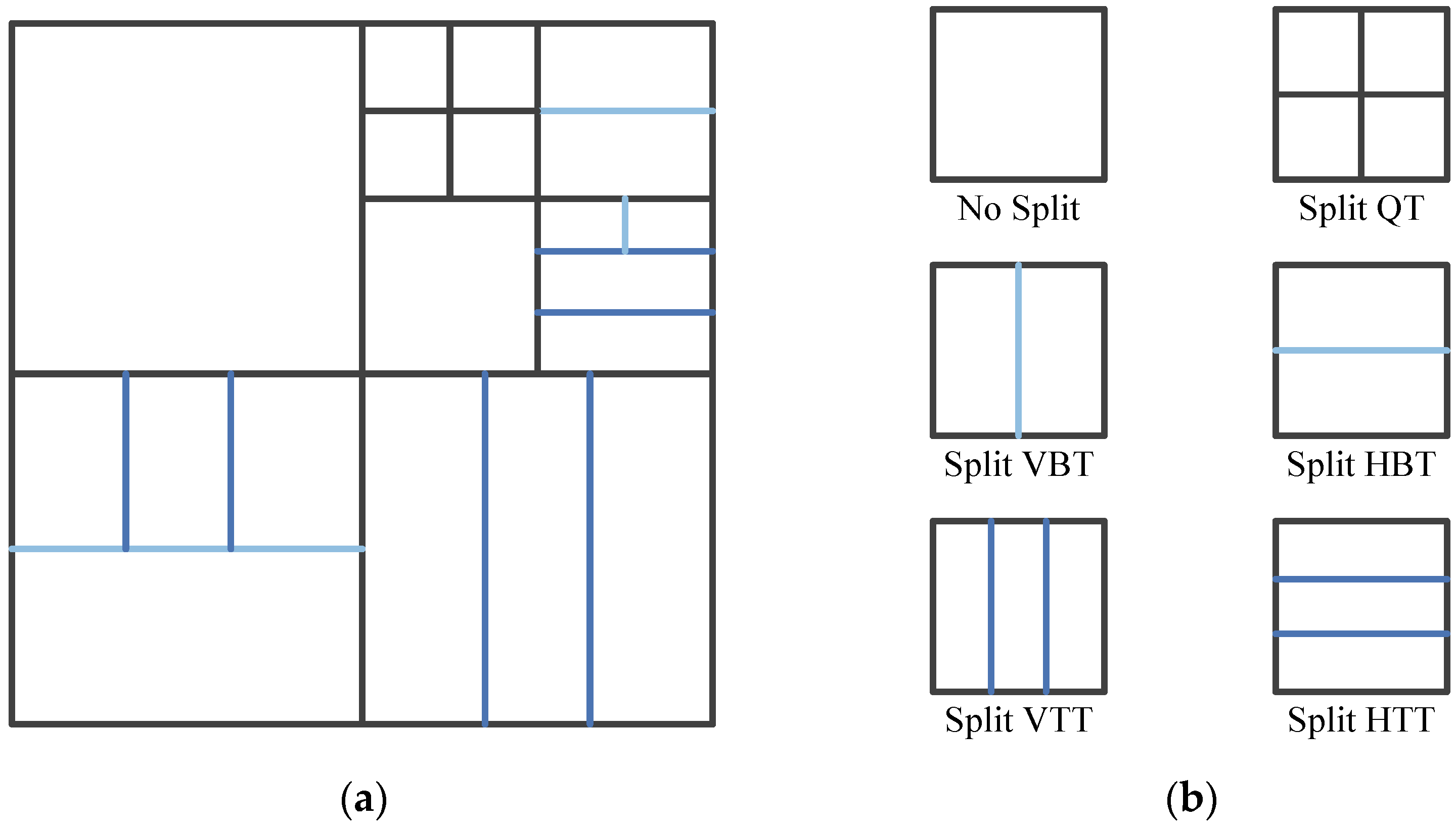
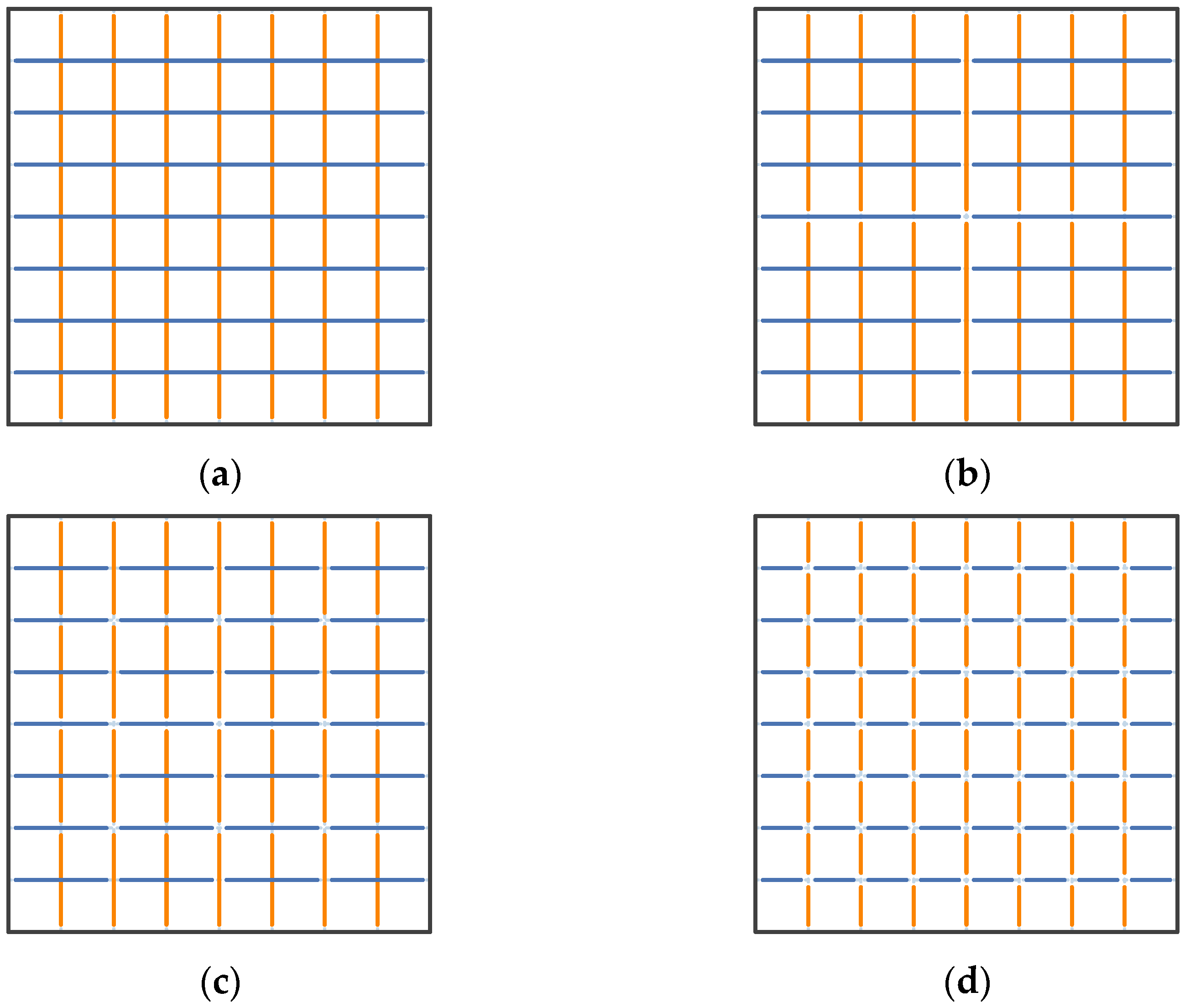
3.1. Stage Grid Map

Since VVC introduces QTMT technology, which leads to diversity in the CU sizes, it is inefficient and time-consuming to directly predict the partitioning process of each CU [26]. Therefore, we propose the concept of a stage grid map, which can directly represent the overall division of CUs with a size of 32 × 32 as the standard output form of the subsequently proposed MET-CNN to realize the overall prediction of the CU division.

Due to the division characteristics of QTMT, in a CU with a size of 32 × 32, there will be division boundaries of different lengths, the shortest being 4 pixels and the longest being 32 pixels. Therefore, according to the length of the division boundary, we divided the division of a 32 × 32 CU into four stages and determined all possible division boundaries at each stage, as shown in Figure 3. Specifically, at Stage 1, due to the length between the two parallel boundaries of at least 4 pixels, there are seven probable division boundaries with a length of 32 pixels in the horizontal and vertical directions respectively, for a total of 14 division boundaries. By analogy, the length of the division boundary at Stage 2 is 16 pixels, and there are 14 horizontal and 14 vertical division boundaries, for a total of 28 division boundaries. At Stage 3, the length of the division boundary is 8 pixels, and there are 28 horizontal and 28 vertical division boundaries, totaling 56. At Stage 4, the length of the division boundary is 4 pixels, and there are 56 division boundaries in the horizontal and vertical directions, totaling 112. Next, we tried to express the division of each stage. A binary label was used to mark the division status of each division boundary. If it was divided, it was marked as “1”, and if it was not divided, it was marked as “0”. The labels of all division boundaries at each stage were formed into a vector, which represents the division information of this stage. Taking the fourth stage as an example, according to the marking principle of vertical first and then horizontal, the first value of the vector represents the first vertical boundary in the first column from the upper left, and the second value represents the second vertical boundary in the first column, and so on. The ninth value represents the first vertical boundary in the second column, the 57th value represents the first horizontal boundary in the first row from the upper left, and the 112th value represents the last horizontal boundary in the seventh row.

The stage grid map vividly embodies the encoding procedure from a larger-size CU to a smaller-size CU in VVC. This map can divide the CU partitioning process into four stages and represent it as a structured output to be used with MET-CNN to achieve a fast CU partitioning process. Furthermore, since the stage grid map contains the full partition information of each 32 × 32 block and its sub-CUs, it can be highly parallelized and is more efficient than previous methods.

A similar idea was also proposed in [23] to predict the division of each 4 × 4 boundary in the CU, which can be viewed as one of the cases of the stage grid map. In contrast, our proposed stage grid map has greater advantages. If the texture complexity of the CU is low, the 14 boundary values in the first stage can be used to represent all its division information, and with MET-CNN, the CU division process can be exited in advance, which greatly saves the coding time. There is no need to predict 480 values for all CUs to represent their partition information as in [23]. At the same time, the inconsistency between the small boundaries also brings great difficulty to the division decision-making process. Stage 4 of the grid map is only enabled when dealing with higher-complexity CUs. Therefore, compared to previous algorithms, the stage grid map can more flexibly handle CUs with different texture complexities and show higher prediction efficiency and better inference performance.

3.2. Multi-Stage Early Termination CNN

Afterward, we designed a MET-CNN to learn a stage grid map for fast decisions on CU partitions. Figure 4 shows the structure of the MET-CNN, which was inspired by the small ResNet [27]. We sampled the 32 × 32 luminance block on the left and above to obtain a 33 × 33 × 1 luminance CU as the input of the MET-CNN. Similar to the stage grid map, the MET-CNN is also divided into four stages, each stage is performed in a series, and each stage provides an output result. The output result is a vector composed of multiple values, and each value represents the probability of whether the corresponding boundary is divided, which is used to cooperate with the stage grid map to make decisions on the division type of the CU at the current stage.

The MET-CNN structure includes the following:

• The backbone of the CNN consists of four stages, each with an output;
• Each stage consists of two set blocks, an average pooling layer with a size of 2 × 2 and a stride of 2, a convolutional layer with a 3 × 3 convolution kernel, a global average pooling layer, and a fully connected layer. The first stage additionally contains a convolutional layer with a 3 × 3 × 16 convolution kernel;
• Each set block contains two convolutional layers with a 3 × 3 × k convolution kernel, a convolutional layer with a 1 × 1 × k convolution kernel, and a shortcut layer. The value of k varies at each stage.

It is important to note that each convolutional layer has a stride of 1 and is activated with a rectified linear unit (ReLU) after each convolutional layer. Batch normalization (BN) was used to speed up convergence during training. The number of fully connected layer nodes at each stage corresponds to the number of boundaries at each stage in the stage grid map. For example, the first stage outputs a vector composed of 14 probability values, the second stage outputs a vector composed of 28 probability values, and so on. The shortcut layer represents the skip connection, which refers to the summation of the characteristic values of the corresponding channels, and does not change the number of channels.

Taking the first stage as an example, the luminance CU of 33 × 33 × 1 was the input, and the feature map of 33 × 33 × 16 was obtained after the convolutional layer of 3 × 3 × 16. Then after two set blocks, the feature map size became 33 × 33 × 32. Then, a feature map of size 16 × 16 × 32 was obtained through the average pooling layer. After going through a convolutional layer with a kernel of 3 × 3 × 32 and a global average pooling layer, a 1 × 1 × 32 feature map was obtained. Finally, through the fully connected layer of 14 nodes, a vector composed of 14 probabilities was obtained, which then cooperated with the decision-making process to complete the division decision of the first stage of CU.

In addition, compared to traditional neural networks, the MET-CNN comes with an early exit mechanism, which indicates that the prediction results from lower stages are likely to exit the neural network and CU partitioning process early. For example, if it is determined that the division result of a 32 × 32 CU is “not divided” according to the predicted value of Stage 1, the calculation processes of Stages 2 to 4 are not performed, and the current CU division process is directly exited, thereby greatly reducing the encoding time.

3.3. Model Training

The datasets used to train the MET-CNN were derived from pictures from the DIV2K dataset [28] and some other databases containing 20M patches. We used VVC’s latest official test software VTM10.0 to encode the dataset with QPs of 22, 27, 32, 37, and AI configuration, respectively, and counted the division information of 32 × 32 CUs. Then it was marked in the form of the stage grid map mentioned in the previous section to form the final dataset used. The MET-CNN architecture was built and trained in Python 4.0 based on the PyTorch learning library. In detail, we used the Adam optimizer for optimization with an initial learning rate of 10^-3 for 300 epochs. The learning rate was updated at a rate of every 50 epochs divided by a factor of 10, and the batch size of the trained model was 128.

The loss function plays an extremely critical role in the training process of a CNN, which may directly affect the performance of the CNN. Therefore, we adopted the cross-entropy function as the loss function when training the MET-CNN. For a single 32 × 32 CU sample m in a batch, the loss function $L_m$ is:

$$L_m=-{\displaystyle \sum _{i=1}^4{\displaystyle \sum _{j=1}^{n_i}{p}_{i,j}\cdot \log (q_{i,j})}}+(1-p_{i,j})\cdot \log (1-q_{i,j}),$$

(3)

where $n_i$ represents the total number of boundaries in the i-th stage; $p_{i,j}$ represents the actual value of the j-th boundary at the i-th stage; similarly, $q_{i,j}$ is the predicted value of the corresponding boundary.

For a batch, the total loss function $Loss$ is the average of all sample loss functions in the batch, and the formula is:

$$Loss=\frac{1}{N}\cdot {\displaystyle \sum _{m=1}^N{L}_m},$$

(4)

where N indicates the number of samples in a batch.

3.4. CU Partition Decision Process

After designing the stage grid map and MET-CNN, we proposed a fast CU partition decision method to make the overall partition decision for CUs with a size of 32 × 32.

As shown in Figure 5, the algorithm flow is for a block with a size of 32 × 32, and with the characteristics of the stage grid map and the MET-CNN, the entire flow is also divided into four stages in a series. For the i-th stage, the detailed algorithm flow is as follows:

• Step 1: Input a luma block of size 32 × 32;
• Step 2: The luminance block is fed into the MET-CNN as input, and it runs to its i-th stage to get the output vector of this stage;
• Step 3: According to the output vector, the probabilities of the five possible division types at this stage are calculated, and the formula is shown in Equations (5)–(9);
• Step 4: The calculated probabilities of the five division types are compared with the set threshold $Th$ in the order of $P_{QT}$, $P_{HBT}$, $P_{VBT}$, $P_{HTT}$, and $P_{VTT}$. The threshold formula is shown in Equation (10). If the probability value of the division type is greater than $Th$, the current stage CU performs the division type corresponding to the probability value and moves to the next stage. If the probability values of all division types are not greater than $Th$, the division process of the CU at the current stage is terminated in advance. Note that if the division result of the first stage is TT division, the decision-making process of the second stage needs to be judged according to the output vector of the third stage.

The division probability formula of VBT is:

$$\{\begin{array}{l}a=2^{S-1}\\ n=\frac{x}{4}+\frac{w}{8}-1\\ i=a\cdot \frac{y}{32}+n\cdot a\\ P_{VBT}=\frac{32}{a\cdot h}\cdot {\displaystyle \sum _{j=1}^{a\cdot h/32}{p}_{i+j}}\end{array},$$

(5)

The division probability formula of HBT is:

$$\{\begin{array}{l}a=2^{S-1}\\ n=\frac{y}{4}+\frac{h}{8}-1\\ i=a\cdot \frac{x}{32}+n\cdot a+7a\\ P_{HBT}=\frac{32}{a\cdot w}\cdot {\displaystyle \sum _{j=1}^{a\cdot w/32}{p}_{i+j}}\end{array},$$

(6)

The division probability formula of VTT is:

$$\{\begin{array}{l}a=2^{S-1}\\ n_1=\frac{x}{4}+\frac{w}{16}-1\\ n_2=\frac{x}{4}+\frac{3}{16}\cdot w-1\\ i_1=a\cdot \frac{y}{32}+n_1\cdot a\\ i_2=a\cdot \frac{y}{32}+n_2\cdot a\\ P_1=\frac{32}{a\cdot h}\cdot {\displaystyle \sum _{j=1}^{a\cdot h/32}{p}_{i_1+j}}\\ P_2=\frac{32}{a\cdot h}\cdot {\displaystyle \sum _{j=1}^{a\cdot h/32}{p}_{i_2+j}}\\ P_{VTT}=Max\left(P_1,P_2\right)\end{array},$$

(7)

The division probability formula of HTT is:

$$\{\begin{array}{l}a=2^{S-1}\\ n_1=\frac{y}{4}+\frac{h}{16}-1\\ n_2=\frac{y}{4}+\frac{3}{16}\cdot h-1\\ i_1=a\cdot \frac{x}{32}+n_1\cdot a+7a\\ i_2=a\cdot \frac{x}{32}+n_2\cdot a+7a\\ P_1=\frac{32}{a\cdot w}\cdot {\displaystyle \sum _{j=1}^{a\cdot w/32}{p}_{i_1+j}}\\ P_2=\frac{32}{a\cdot w}\cdot {\displaystyle \sum _{j=1}^{a\cdot w/32}{p}_{i_2+j}}\\ P_{HTT}=Max\left(P_1,P_2\right)\end{array},$$

(8)

The division probability formula of QT is:

$$P_{QT}=\frac{1}{2}\left(P_{VBT}+P_{HBT}\right),$$

(9)

where $S$ denotes the number of stages in the current MET-CNN run; $x$ and $y$ indicate the coordinates of the upper left corner of the current stage CU in a 32 × 32 size block; $h$ and $w$ denote the height and width of the current stage CU, respectively; $p_{i+j}$ represents the probability value that the sequence number in the output vector is the i + jth.

In terms of the selection of the threshold, considering that the size of the CU at different stages is different, if the threshold remains unchanged, it will affect the final decision-making result. Therefore, we adopted a dynamic threshold. A smaller threshold was used for high-stage CUs, and a larger threshold was used for low-stage CUs, which can achieve better decision-making effects. The threshold formula is as follows:

$$Th=a-b\cdot S,$$

(10)

where $S$ indicates the number of stages in the current MET-CNN run; a, b are fixed constants, which can be {(a, b)|(0.9, 0.1),(0.9, 0.2),(0.9, 0.3),(0.8, 0.1),(0.8, 0.2),(0.8, 0.3),(0.7, 0.1),(0.7, 0.2),(0.7, 0.3)}. In order to select the most suitable threshold, we used the overall algorithm with different threshold formulas to perform coding tests on the VVC standard test sequence ParkRunning3 under the coding environments of QP = 22, 27, 32, and 37. The algorithm performance is listed under different thresholds in

Table 2. Algorithm performance at different thresholds.

(a, b)	BDBR (%)	ΔT (%)
(0.9, 0.1)	0.73	39.29
(0.9, 0.2)	0.99	49.36
(0.9, 0.3)	1.32	55.64
(0.8, 0.1)	0.95	54.58
(0.8, 0.2)	0.98	50.69
(0.8, 0.3)	1.09	53.23
(0.7, 0.1)	0.96	49.69
(0.7, 0.2)	1.10	54.12
(0.7, 0.3)	1.14	56.31

. The performance of the algorithm was measured using ΔT and the Bjøntegaard Delta Bit Rate (BDBR). ΔT represents the coding time-saving rate of the proposed algorithm compared with the original VTM10.0 algorithm, which was used to measure the performance of reducing complexity. BDBR was used to measure the RD performance.

$$\Delta T=\frac{1}{4}\cdot {\displaystyle \sum _{i\in QP}\frac{T_{base}(Q{P}_i)-T_{prop}(Q{P}_i)}{T_{base}(Q{P}_i)}}\cdot 100\%,$$

(11)

where $T_{base}(Q{P}_i)$ and $T_{prop}(Q{P}_i)$ indicate the encoding time spent by the original algorithm and the algorithm proposed in this paper under QP = 22, 27, 32, and 37, respectively.

According to the results shown in Table 2, we finally set (a, b) to be (0.8, 0.1), so that the proposed algorithm can achieve the best performance. The final threshold formula is:

$$Th=0.8-0.1\cdot S,$$

(12)

where $S$ indicates the number of stages in the current MET-CNN run.

A fast CU partition decision algorithm for VVC intra coding based on an MET-CNN is proposed in this article. The algorithm can achieve the division decision of a 32 × 32 CU and all its sub-CUs by using the CNN model only once, and completely skipping the tedious RDO, thus greatly reducing the computational complexity. In addition, each stage in the algorithm is performed in series, and each stage outputs a prediction result, which is used to make a decision on the CU of the current stage. Furthermore, the algorithm has an early termination mechanism. For a complex CU, only the prediction of the lower stage can be performed to obtain the division result, skip the prediction process of the higher stage, and terminate the division decision process in advance, thereby further reducing the coding time.

4. Experimental Results

4.1. Experimental Environment

All experiments were performed under the AI configuration environment in VVC’s latest encoder version VTM10.0. The MET-CNN architecture was built and tested in Python 4.0 based on the PyTorch learning library, and each encoding and MET-CNN prediction was run on an Intel Core i5-8500 [email protected] processor in the Windows 10 operating system. We selected 18 CTC standard test sequences with different resolutions, video content, and texture complexity, which were divided into five categories: A1(4K), A1 (4K), B (1920 × 1080), C (832 × 480), D (416 × 240), and E (1280 × 720). The above test sequences formed a test set to test the performance of the suggested algorithm. In the experiment, we tested the test set with the fast algorithm suggested in this article under the coding environments of QP = 22, 27, 32, and 37, and averaged the experimental data to obtain the experimental results. It should be emphasized that the construction and training of the MET-CNN were both offline processes, so the time spent was not included in the encoding time.

We chose two criteria to measure the performance of the proposed method, ΔT and BDBR. ΔT represents the coding time-saving rate of the proposed algorithm compared with the original VTM10.0 algorithm, which was used to measure the performance of reducing complexity. BDBR was used to measure the RD performance.

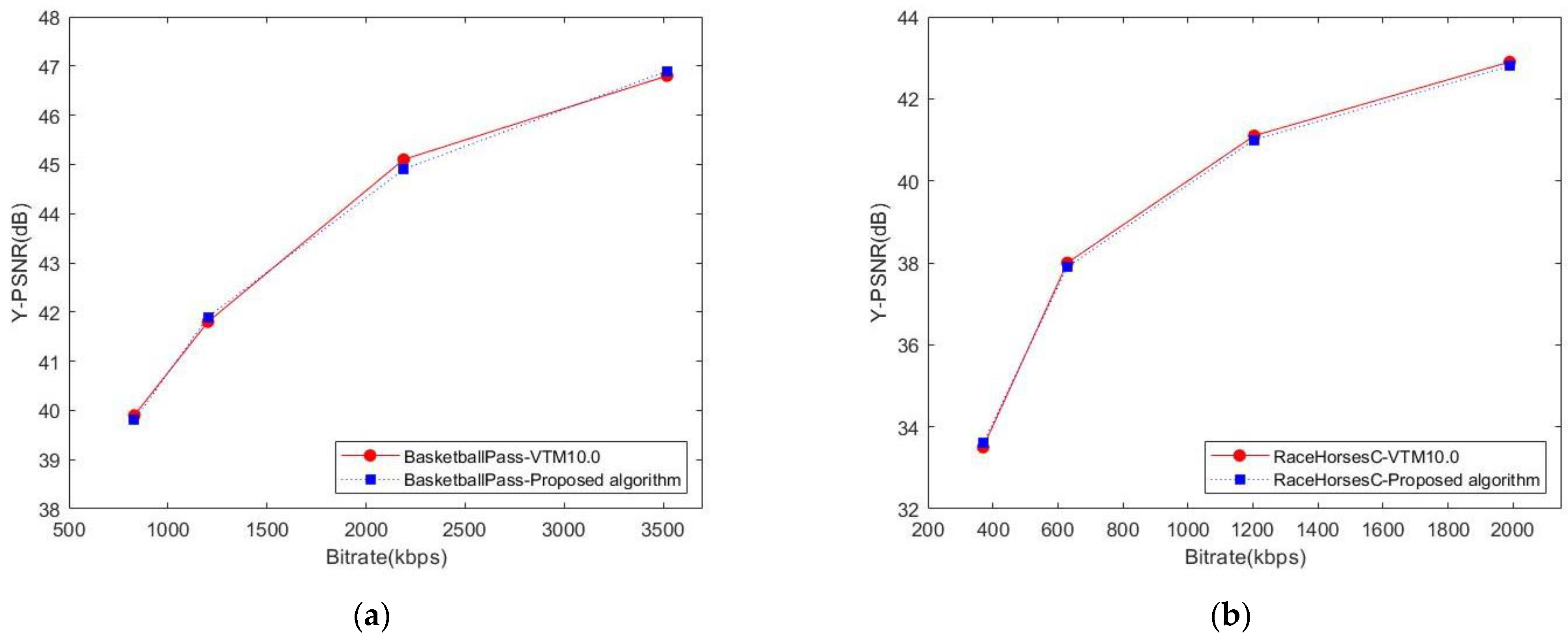
4.2. Analysis of Experimental Results

To prove the effectiveness of the method proposed in this article, we utilized the method proposed in this article and the current more advanced fast CNN-based algorithm ([21,26]) to perform coding experiments under the same sequence, same configuration (AI), and the same parameters. Then, we compared it to the original algorithm of VTM10.0, and the experimental results are shown in

Table 3. Performance of the proposed algorithm.

Test Sequence		[26]		[21]		Proposed
		BDBR (%)	ΔT (%)	BDBR (%)	ΔT (%)	BDBR (%)	ΔT (%)
Class A1 4K	FoodMarket4	3.35	27.09	0.22	29.94	0.57	40.62
	Campfire	2.81	25.71	0.81	45.62	0.82	55.78
Class A2 4K	Catrobot1	2.50	28.34	0.80	44.50	1.35	53.63
	DaylightRoad2	2.59	32.96	0.72	45.95	0.75	50.21
	ParkRunning3	1.96	21.93	0.47	43.84	0.95	54.58
Class B 1920 × 1080	Cactus	3.99	22.78	0.72	46.77	1.31	56.87
	BasketballDrive	6.79	20.67	0.67	48.98	0.83	54.23
	BQTerrace	4.80	25.91	0.60	41.75	0.91	50.67
Class C 832 × 480	BasketballDrill	2.95	28.37	1.40	37.63	1.17	44.39
	BQMall	5.70	21.69	0.89	41.72	1.12	49.47
	PartyScene	2.80	20.89	0.28	38.73	0.98	47.02
	RaceHorsesC	3.70	21.43	0.61	43.39	0.67	48.15
Class D 416 × 240	BasketballPass	5.46	22.29	0.62	38.06	1.01	49.11
	BQsquare	2.36	26.62	0.44	32.56	0.87	40.61
	BlowingBubbles	2.69	27.78	0.32	36.97	1.16	48.91
	RaceHorses	3.32	25.71	0.45	36.86	0.68	44.28
Class E 1280 × 720	FourPeople	6.73	21.82	1.08	42.57	0.88	46.82
	KristenAndSara	8.82	23.68	1.00	45.53	1.53	50.94
Average		4.07	24.76	0.67	41.18	0.97	49.24

.

The experimental results demonstrate that, compared to the original VTM10.0 algorithm, our proposed algorithm reduced the coding complexity by 49.24% on average, and led to only a 0.97% increase in BDBR (negligible). Among them, for different categories, the algorithm proposed in this article had the best performance in reducing complexity in Class A2 and Class B, reducing the coding times by 52.81% and 53.92% on average. This shows that the suggested algorithm can have better performance when targeting higher-resolution sequences. For a single sequence, the proposed algorithm decreased the encoding time by a maximum of 56.87% (Cactus) and by a minimum of 40.61% (BQsquare). This demonstrates that the proposed algorithm is universal and effective at reducing coding complexity and can perform well for all sequences. Since the proposed algorithm can completely replace the complex RDO process and complete the CU partition decision, and the result of the partition prediction is basically similar to that of the original algorithm, the algorithm proposed in this paper can greatly reduce the encoding time on the premise of maintaining the encoding quality.

Compared to the current more advanced fast algorithms based on a CNN, the algorithm proposed in this article also shows obvious advantages. Among them, compared to [26], the proposed algorithm had better performance both in terms of decreasing the coding complexity and the RD performance. On average, the encoding time was reduced by 24.48% compared to the algorithm in [26], and the BDBR was also reduced by an average of 3.1%. Especially in the sequence Cactus, this result is more obvious, showing that the complexity was reduced by as much as 34.09% compared to [26]. We can conclude that when the proposed algorithm was encoded for different sequences and different categories, its complexity reduction performance and RD performance improvements were huge compared to [26].

Compared to [21], the proposed method reduced the encoding time by 8.06% on average, and the BDBD only increased by 0.3%. Especially in the sequence BlowingBubbles, this result is more obvious, showing that the complexity was reduced by as much as 11.94% compared to [21]. Specifically, the algorithm proposed in this paper shows better performance both in higher resolution categories such as Class A1 and Class A2 and in lower resolution categories, such as Class C and Class D (in Class A1, the encoding time decreased by an average of 10.42% compared to [21]; in Class D, the encoding time decreased by an average of 9.62% compared to [21]).

In addition, to better see the RD performance of the proposed algorithm, we selected the video sequences BasketballPass and RaceHorsesC from different categories. Then we used the original VTM10.0 algorithm and the method suggested in this article to conduct coding experiments and compared the RD performance of the two, as shown in Figure 6. From Figure 6, we can draw the conclusion that the RD curve of the suggested algorithm basically coincides with the RD curve of the original algorithm of VTM10.0. This shows that the proposed algorithm can substantially achieve the same encoding quality as the original algorithm, while greatly saving encoding time and achieving a better balance between encoding complexity reduction and RD performance.

To sum up, the fast CU partition decision algorithm for VVC intra coding based on the MET-CNN suggested in this article, whether compared to the original VTM10.0 algorithm or other advanced excellent algorithms at present, shows more promising performance in terms of coding complexity reduction. Meanwhile, the loss of coding quality is small and almost negligible, effectively realizing the balance between coding complexity reduction and RD performance.

5. Conclusions

In this article, we first propose a stage grid map that divides the overall partitioning of a 32 × 32 CU into four stages and represents it as a structured output. Second, a MET-CNN model was designed to predict the full partition information of a CU of size 32 × 32. Finally, a fast CU partition decision-making process is proposed, which can predict all the partition information of a CU with a size of 32 × 32 and its sub-CUs by running the algorithm only once, completely replacing the complex RDO process. It also has an early exit mechanism, thus greatly reducing computational complexity and saving coding time. The experimental results demonstrate that the algorithm proposed in this article reduces the encoding time by 49.24% on average, and the BDBR only raises by 0.97% (negligible). The results prove that the proposed algorithm can greatly reduce the coding complexity of VVC, save coding time, and achieve an effective balance between coding complexity reduction and RD performance.

References

1. Qian, X.; Zeng, Y.; Wang, W.; Zhang, Q. Co-saliency Detection Guided by Group Weakly Supervised Learning. IEEE Trans. Multimed. 2022, 1, 1. [Google Scholar] [CrossRef]
2. Oh, K.; So, J.; Kim, J. Low complexity implementation of slim—HEVC encoder design. In Proceedings of the 2016 International Conference on Systems, Signals and Image Processing (IWSSIP), Bratislava, Slovakia, 23–25 May 2016; pp. 1–4. [Google Scholar]
3. Filippov, A.; Rufitskiy, V.; Chen, J.; Alshina, E. Intra Prediction in the Emerging VVC Video Coding Standard. In Proceedings of the 2020 Data Compression Conference (DCC), Snowbird, UT, USA, 24–27 March 2020; p. 367. [Google Scholar]
4. Versatile Video Coding, Recommendation ITU-T H.266 and ISO/IEC 23090-3 (VVC), ITU-T and ISO/IEC JTC. 1 July 2020. Available online: http://phenix.it-sudparis.eu/jvet/doc_end_user/current_document.php?id=10399 (accessed on 6 August 2022).
5. Ye, Y.; Boyce, J.M.; Hanhart, P. Omnidirectional 360° Video Coding Technology in Responses to the Joint Call for Proposals on Video Compression with Capability Beyond HEVC. IEEE Trans. Circuits Syst. Video Technol. 2020, 30, 1241–1252. [Google Scholar] [CrossRef]
6. Huang, Y.-W. Block Partitioning Structure in the VVC Standard. IEEE Trans. Circuits Syst. Video Technol. 2021, 31, 3818–3833. [Google Scholar] [CrossRef]
7. Bouaafia, S.; Khemiri, R.; Sayadi, F.E. Rate-Distortion Performance Comparison: VVC vs. HEVC. In Proceedings of the 2021 18th International Multi-Conference on Systems, Signals & Devices (SSD), Monastir, Tunisia, 22–25 March 2021; pp. 440–444. [Google Scholar]
8. Chen, Z.; Shi, J.; Li, W. Learned Fast HEVC Intra Coding. IEEE Trans. Image Processing 2020, 29, 5431–5446. [Google Scholar] [CrossRef] [PubMed]
9. Lilhore, U.K.; Imoize, A.L.; Lee, C.C.; Simaiya, S.; Pani, S.K.; Goyal, N.; Kumar, A.; Li, C.T. Enhanced convolutional neural network model for cassava leaf disease identification and classification. Mathematics 2022, 10, 580. [Google Scholar] [CrossRef]
10. Zhang, G.; Xiong, L.; Lian, X.; Zhou, W. A CNN-based Coding Unit Partition in HEVC for Video Processing. In Proceedings of the 2019 IEEE International Conference on Real-Time Computing and Robotics (RCAR), Irkutsk, Russia, 4–9 August 2019; pp. 273–276. [Google Scholar]
11. Liu, Y.; Wei, A. A CU Fast Division Decision Algorithm with Low Complexity for HEVC. In Proceedings of the 2020 IEEE 4th Information Technology, Networking, Electronic and Automation Control Conference (ITNEC), Chongqing, China, 12–14 June 2020; pp. 1028–1032. [Google Scholar]
12. Guo, X.; Wang, Q.; Jiang, J. A Lightweight CNN for Low-Complexity HEVC Intra Encoder. In Proceedings of the 2020 IEEE 15th International Conference on Solid-State & Integrated Circuit Technology (ICSICT), Kunming, China, 3–6 November 2020; pp. 1–3. [Google Scholar]
13. Jamali, M.; Coulombe, S.; Sadreazami, H. CU Size Decision for Low Complexity HEVC Intra Coding based on Deep Reinforcement Learning. In Proceedings of the 2020 IEEE 63rd International Midwest Symposium on Circuits and Systems (MWSCAS), Springfield, MA, USA, 9–12 August 2020; pp. 586–591. [Google Scholar]
14. Kim, K.; Ro, W.W. Fast CU Depth Decision for HEVC Using Neural Networks. IEEE Trans. Circuits Syst. Video Technol. 2019, 29, 1462–1473. [Google Scholar] [CrossRef]
15. Heindel, A.; Haubner, T.; Kaup, A. Fast CU split decisions for HEVC inter coding using support vector machines. In Proceedings of the 2016 Picture Coding Symposium (PCS), Nuremberg, Germany, 4–7 December 2016; pp. 1–5. [Google Scholar]
16. Zhang, Y.; Kwong, S.; Wang, X.; Yuan, H.; Pan, Z.; Xu, L. Machine Learning-Based Coding Unit Depth Decisions for Flexible Complexity Allocation in High Efficiency Video Coding. IEEE Trans. Image Processing 2015, 24, 2225–2238. [Google Scholar] [CrossRef] [PubMed]
17. Javaid, S.; Rizvi, S.; Ubaid, M.T.; Tariq, A. VVC/H.266 Intra Mode QTMT Based CU Partition Using CNN. IEEE Access 2022, 10, 37246–37256. [Google Scholar] [CrossRef]
18. HoangVan, X.; NguyenQuang, S.; DinhBao, M.; DoNgoc, M.; Trieu Duong, D. Fast QTMT for H.266/VVC Intra Prediction using Early-Terminated Hierarchical CNN model. In Proceedings of the 2021 International Conference on Advanced Technologies for Communications (ATC), Ho Chi Minh City, Vietnam, 14–16 October 2021; pp. 195–200. [Google Scholar]
19. Zhao, J.C.; Wang, Y.H.; Zhang, Q.W. Fast CU Size Decision Method Based on Just Noticeable Distortion and Deep Learning. Sci. Program. 2021, 2021, 3813116. [Google Scholar] [CrossRef]
20. Li, T.; Xu, M.; Tang, R.; Chen, Y.; Xing, Q. DeepQTMT: A Deep Learning Approach for Fast QTMT-Based CU Partition of Intra-Mode VVC. IEEE Trans. Image Processing 2021, 30, 5377–5390. [Google Scholar] [CrossRef] [PubMed]
21. Fu, P.-C.; Yen, C.-C.; Yang, N.-C.; Wang, J.-S. Two-phase Scheme for Trimming QTMT CU Partition using Multi-branch Convolutional Neural Networks. In Proceedings of the 2021 IEEE 3rd International Conference on Artificial Intelligence Circuits and Systems (AICAS), Washington, DC, USA, 6–9 June 2021; pp. 1–6. [Google Scholar]
22. Tang, G.; Jing, M.; Zeng, X.; Fan, Y. Adaptive CU Split Decision with Pooling-variable CNN for VVC Intra Encoding. In Proceedings of the 2019 IEEE Visual Communications and Image Processing (VCIP), Sydney, NSW, Australia, 1–4 December 2019; pp. 1–4. [Google Scholar]
23. Tissier, A.; Hamidouche, W.; Vanne, J.; Galpin, F.; Menard, D. CNN Oriented Complexity Reduction Of VVC Intra Encoder. In Proceedings of the 2020 IEEE International Conference on Image Processing (ICIP), Abu Dhabi, United Arab Emirates, 25–28 October 2020; pp. 3139–3143. [Google Scholar]
24. Zhang, Q.; Guo, R.; Jiang, B.; Su, R. Fast CU Decision-Making Algorithm Based on DenseNet Network for VVC. IEEE Access 2021, 9, 119289–119297. [Google Scholar] [CrossRef]
25. Huang, Y.-H.; Chen, J.-J.; Tsai, Y.-H. Speed Up H.266/QTMT Intra-Coding Based on Predictions of ResNet and Random Forest Classifier. In Proceedings of the 2021 IEEE International Conference on Consumer Electronics (ICCE), Las Vegas, NV, USA, 10–12 January 2021; pp. 1–6. [Google Scholar]
26. Abdallah, B.; Belghith, F.; Ben Ayed, M.A.; Masmoudi, N. Low-complexity QTMT partition based on deep neural network for Versatile Video Coding. Signal Image Video Processing 2021, 15, 1153–1160. [Google Scholar] [CrossRef]
27. He, K.; Zhang, X.; Ren, S.; Sun, J. Deep Residual Learning for Image Recognition. In Proceedings of the 2016 IEEE Conference on Computer Vision and Pattern Recognition (CVPR), Las Vegas, NV, USA, 27–30 June 2016; pp. 770–778. [Google Scholar]
28. Agustsson, E.; Timofte, R. NTIRE 2017 Challenge on Single Image Super-Resolution: Dataset and Study. In Proceedings of the 2017 IEEE Conference on Computer Vision and Pattern Recognition Workshops (CVPRW), Honolulu, HI, USA, 21–26 July 2017; pp. 1122–1131. [Google Scholar]
Figure 1. CU partitioning in VVC: (a) 64 × 64 CU as an example; (b) VVC split types.
Electronics 11 03090 g001
Figure 2. Comparison diagram of CU division of different coding standards. (a) In VVC; (b) in HEVC.
Electronics 11 03090 g002
Figure 3. Stage grid map. N is the number of boundaries in the current stage; L is the boundary length in the current stage; Blue and orange represent horizontal and vertical division boundaries, respectively. (a) Stage 1, N = 14, L = 32; (b) Stage 2, N = 28, L = 16; (c) Stage 3, N = 56, L = 8; (d) Stage 4, N = 112, L = 4.
Electronics 11 03090 g003
Figure 4. Structure diagram of the proposed MET-CNN model.
Electronics 11 03090 g004
Figure 5. Flowchart of CU partition decision based on MET-CNN. (a) Overall flow chart; (b) detailed flowchart of the i-th stage.
Electronics 11 03090 g005
Figure 6. RD performance comparison chart of the proposed algorithm. (a) RD of the BasketballPass; (b) RD of the RaceHorsesC.
Electronics 11 03090 g006