Abstract
The integration of sensing, computing, storage, and communications is one of the main research directions of current network development. To achieve the integration, an innovative design in the antenna array is essential. This paper presents a novel design of an irregularly distributed antenna array for smart 6G networks. Firstly, to solve the problem of fast amplitude and phase distribution of conformal arrays, the fast electromagnetic code of the multilevel fast multipole (MLFMA) based on volume surface integral equations (VSIE) is used to simulate the radiation characteristics of the irregularly distributed antenna arrays. Secondly, another stochastic global optimization algorithm, Simulated Annealing (SA), has been widely used to solve multiscale nonlinear problems. Finally, the performance of the proposed antenna array is given by simulation results and tests, to prove the effectiveness and correctness.
1. Introduction
In past communication systems, communication, sensing, and computation existed independently of each other. Such an individual-based design results in a waste of wireless resources. Integrating sensing, computing, and communication can achieve joint resource scheduling in 6G networks. Meanwhile, in the next generation network, the smart antenna system is responsible for the critical task of receiving and transmitting electromagnetic waves [1]. It can be widely used in 6G systems by sending electromagnetic waves into space and subsequently using the scattered electromagnetic waves from the target to accomplish tasks such as detection and localization [2]. In the continuous development of antenna systems today, the requirements for modern antennas are getting higher and higher. To achieve integration, an innovative design in the antenna array is essential. As phased array antennas have the characteristics of high gain, narrow beam, and the beam can be electrically scanned, they have become the current hotspot of plans for integrating sensing, computing, storage, and communications towards intelligent 6G networks [3]. Phased array antennas are not only deployed on ground devices, but high-frequency phased array antennas with miniaturized components are also widely used on aircrafts, satellites, and various missiles [4].
Phased array antenna beam control, as one of the critical technologies, directly affects the accuracy. Large antenna arrays have been widely used because of their advantages, such as high beam directivity and their low first range side lobe level (FSLL). To reduce the complexity and cost of the array, subarray technology is usually used in extensive array synthesis.
The distributed array is a further developed form of phased array, consisting of multiple subarrays in a decentralized arrangement [5]. Distributed array antennae can split each subarray, splitting the single aperture of the centralized antenna array into individual gaps, breaking the restriction of array element spacing of less than half a wavelength. The distributed array has many advantages, such as better mobility, flexibility, and economy. Distributed arrays can achieve the desired aperture size or performance index by changing the subarray position and excitation. Combining optimization algorithms with subarray phased array technology can effectively suppress grating lobe and high side lobe clutter while maintaining high gain and high beam directivity of the antenna array, significantly reducing the hardware cost and system complexity [6].
Conformal arrays are more widely used than planar arrays because they have the same aerodynamic shape as the carrier and have wide-angle scanning characteristics [7]. A conformal array is usually a non-planar, conformal antenna with a specific object shape, usually as part of the surface of a high-speed moving object. The shape of the array is not determined by electromagnetic factors but by factors such as aerodynamic or hydrodynamic forces [8]. The conformal arrays can therefore avoid the creation of additional aerodynamic drag and improve flight capability accordingly. In addition, there are few locations where a large, high-gain antenna array can be mounted [9]. A conformal array can achieve a larger effective aperture on a limited physical space and avoid conflicting mounting locations.
Therefore, applying subarray technology and optimization algorithms to optimize the shape of the distributed phased array antenna can significantly reduce system complexity and cost and maintain beam flexibility to a large extent, ultimately achieving multi-band, multi-angle composite detection and guidance capability.
2. System Model
2.1. Multilevel Fast Multipole Fast Electromagnetic Calculation
To solve the problem of fast amplitude and phase distribution of conformal arrays, the fast electromagnetic code of the multilevel fast multipole (MLFMA) based on volume–surface integral equations (VSIE) is used to simulate the radiation characteristics of the irregularly distributed antenna arrays. Due to the large computational scale, the core of the simulation algorithm is the volume–surface integral equation (VSIE) based on the method of moments to solve the problem efficiently. These integral equations are particularly suitable for simulating metal-media composite targets with delicate structures. To reduce the complexity of the algorithm, the multilevel fast multipole technique (MLFMA) is used to reduce the computational complexity of the numerical solution of the integral equation from the order of to the order of , where N is the number of unknown quantities. To further accelerate the computation speed, a hybrid parallel computing technique based on MPI and OpenMP mechanisms and a hardware acceleration technique based on a vector logic computing unit (VALU) is used to form a hybrid MPI-OpenMP-VALU parallel program, which can achieve a speedup ratio of more than a hundred times compared with the traditional serial program on a 4-node 64-core server. We reduced storage memory using Spherical Harmonic Expansion (SHE), which reduces the memory occupied by storing directional graph functions in MLFMA to less than a quarter of its previous size. The sparse approximation inverse (SPAI)-based preconditioning technique speeds up the convergence of the iterative solution and combines this technique with the grouping approach of the multilevel fast multipole algorithm, which makes the preconditioning computation much faster.
In the process of comprehensive optimization of the radiation direction map of the array, it is necessary to use the active direction map of each subarray in the array, so the direction map needs to be calculated for both frequency bands of the subarray excited at different aperture positions. In the calculation, two cases are considered: one is the case where the subarray does not have the unit-level phase modulation capability, i.e., the maximum radiation direction map of the subarray always points to the side emission direction; the other is the case where the subarray has the unit-level phase modulation capability in the direction perpendicular to the bullet axis, i.e., the subarray has scanning capability in the H-plane. Therefore, in the range of 0–60 degree scanning angles in the H-plane, the calculation of the directional map of the array needs to be performed at every 10-degree scanning angle increment. For the ultra-wideband array of 2–18 GHz, the specific frequency points selected are 2, 6, 10, 14, and 18 GHz for a total of 5 frequency points; for the ultra-wideband array of 26–40 GHz, the specific frequency points selected are 26, 29.5, 33, 36.5, and 40 GHz for a total of 5 frequency points. Therefore, for the ultra-wideband array, a total of 42 × 5 × 7 = 1470 subarray directional maps need to be calculated; for the K/Ka array, 42 × 5 × 7 = 1470 subarray, directional maps also need to be calculated. It is evident that the computational volume is huge.
After the first optimization step, i.e., determining the subarray position, two methods will be used to optimize the array’s amplitude–phase at different scan angles: the first one is to directly use the subarray active directional map without a subarray-level scanning capability for synthesis; the other is to synthesize the subarray active pattern with the scanning capability of the subarray within the H plane; therefore, since the scanning angles selected for both arrays are 0, 10, 20, 30, 40, 50, and 60 degrees, and 7 other typical scanning angles, a total of 2 (array type) × 7 (standard value of scanning angle) × 5 (number of frequency points) = 70 scanning states of the subarray-level amplitude-phase synthesis and optimization.
After the planar array is completed, the synthesis optimization of the conformal array is also required. For comparison with the planar sparse array, the position distribution in the synthesis of the conformal sparse microstrip array is the same as that of the planar sparse array. Then, the amplitude and phase of the subarray excitation are obtained using the improved simulated annealing (ISA) algorithm to optimize the directional map of the subarray with scanning capability in the H-plane. Since the conformal array increases the array folding angle as an optional variable compared with the planar array, the degree of freedom in array optimization increases, and the optimization scheme increases. Three typical array folding angles (10°, 30°, and 60°) are considered for practical applications, and two folding planes work simultaneously. The axial projectile direction is consistent with the planar array for the Y-axis, and a total of six cell positions are distributed in this direction, two cell positions are distributed in the X-direction for each of the two folding surfaces, and three cell positions are distributed in the middle planar part. Unlike the optimized planar array orientation diagram, which is used in the planar array to synthesize the orientation diagram in the array corresponding to all positions, the computation is too large in the conformal array due to the addition of the folding surface degrees of freedom. It is necessary to use the orientation diagram in the planar array located in the fourth row and third column instead of the element factor, calculate the array factor according to the location of the array element, and use the Eulerian rotation transform.
The overall optimization process is shown in the following Figure 1.
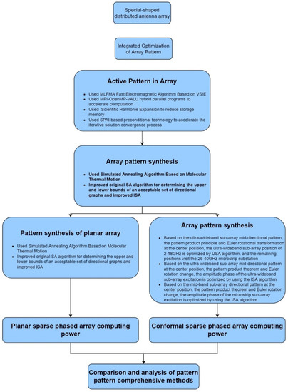
Figure 1.
Optimization process diagram of calculation method.
2.2. Directional Graph Synthesis Algorithm Based on Simulated Annealing Technique
Another stochastic global optimization algorithm, simulated annealing (SA), has been widely used to solve multiscale nonlinear problems. The SA algorithm is highly feasible in optimizing multiple directional map parameters simultaneously. This algorithm was first proposed in 1983 by S. Kirkpatrick, C. D. Gelatt, and M. P. Vecchi and was derived concerning molecular motion in nature. Annealing in simulated annealing refers to the thermal movement of molecules that occurs in a solid such as a metal. The basic idea is that at a specific temperature, the searching molecule can jump randomly from one state to another, accepting the new state with a certain definite probability at higher temperatures according to the Metropolis criterion. At the same time, the search process eventually settles to the optimal solution with a probability of 1 as the temperature keeps dropping to the lowest temperature.
Applying the simulated annealing algorithm to the directional graph synthesis, the temperature can be taken as the control parameter, the state space of the molecule corresponds to the solution space of the required unit excitation coefficient W, and the energy state function of the molecule corresponds to the adaptive function of the solution space. The energy ground state corresponds to the minimum of the adaptive function. Synthesizing the directional diagram can be seen as solving for the unitary excitation coefficient W when takes the minimum value.
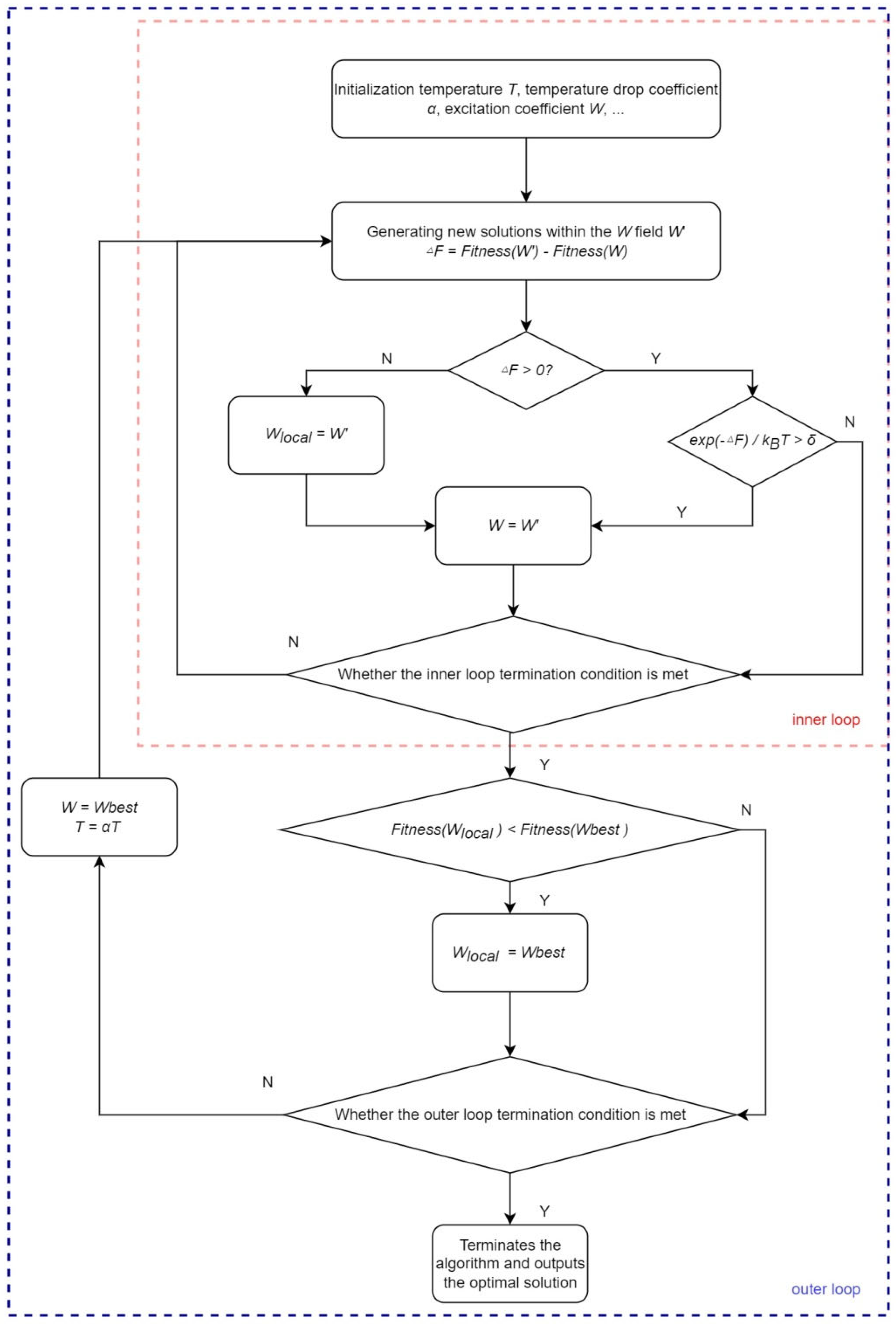
Let the array cell excitation coefficient (molecular state) be W, and the adaptive function (energy state function) be at temperature T. When a new state is generated in the neighborhood of the molecular state W, the new adaptive function is at this time, and acceptance of the new molecular state is judged according to the Metropolis criterion: if accepted, W is replaced by and the current adaptive function is ; if not accepted, the original molecular state is retained, and the corresponding adaptive function is . At this point, determine whether the molecule reaches thermal equilibrium at temperature . If not, regenerate and repeat the application of the Metropolis criterion until the molecule reaches thermal equilibrium; if it reaches thermal equilibrium, cool down and repeat the above steps until the temperature drops to the lowest temperature, at which time the energy of the molecule reaches the ground state and the value of the adaptive function. If the thermal equilibrium state is reached, the above steps are repeated again until the temperature drops to the lowest temperature. The above analysis shows that the SA algorithm can be divided into two layers of inner and outer loops for iterative calculations. The specific flow of the SA algorithm for directional map synthesis is as follows.
As in Figure 2, the iterative computational process can be divided into six steps.
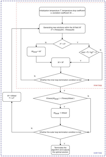
Figure 2.
SA algorithm flow chart.
- (1)
- Initialization
Determine the starting temperature and the temperature drop factor ; determine the adaptive function ; determine the maximum number of iteration steps of the inner loop and the maximum number of iterative steps of the outer loop ; initialize the excitation coefficient , the current optimal solution , and the global optimal solution at the starting temperature to get . The excitation coefficient is independent of . The array element pattern multiplying the array in the line array to obtain the achievable pattern is:
Determine the upper bound of the set according to the range of the set of acceptable directional maps and lower boundaries .
- (2)
- Internal circulation
is generated by the excitation coefficient W according to the following equation:
Among them, the and are two sets of random numbers that are relatively independent and belong to, which represent the values of excitation coefficients; amplitude and phase changes are independent of each other. Subsequently, by normalizing, the modal values are between them.
- (3)
- Metropolis Guidelines Judgment
Specify the difference of the adaptive function values as , and then use the Metropolis criterion to determine whether to update the excitation coefficient as :
- If , then update the excitation coefficient to, such that and update the current optimal solution ;
- If , the excitation coefficient can also be updated if the following acceptance probabilities are satisfied by :where 𝑘𝐵 is the Boltzmann constant, the , and 𝛿 is a random number that takes values in the range (0,1). If the above equation is satisfied, then let ;
- If none of the above conditions are satisfied, then keep the current excitation coefficient and the optimal solution under the current T unchanged.
- (4)
- Inner loop termination judgment
When the inner loop reaches the maximum number of iteration steps 𝑀1 or the value of the adaptive function within consecutive L steps is satisfied with little change, i.e.,
where 𝑀𝐿 is the solution updated by the third step of the Metropolis criterion judgment when the inner loop proceeds to the Lth step, and 𝜀 is the maximum acceptable change in the human-predetermined adaptive value. If any of the internal loop termination conditions are not satisfied, return to step 2 until one of the inner loop termination conditions is satisfied.
- (5)
- External Circulation
If the inner loop termination condition is satisfied, the inner loop is terminated and the outer loop is entered simultaneously. First, compare the optimal solution at the current temperature T and the global optimal solution of the adaptive function values.
- If , then the is updated to ;
- If , then maintain remains unchanged.
- (6)
- External loop termination judgment
Similar to the inner loop termination condition, the outer loop termination condition can be set to when the outer loop reaches the maximum number of iteration steps 𝑀2 or when the value of is less than the preset convergence value. Suppose any of the outer loop termination conditions are not satisfied. In that case, the current temperature T decreases to α𝑇 while initializing , then return to step 2 to reiterate until any of the outer loop termination conditions is satisfied; if any of the outer loop termination conditions are successfully satisfied, the optimal solution of the excitation coefficient is output 𝑊𝑏𝑒𝑠𝑡 and according to output on the final array orientation map.
Based on the above process, it can be seen that determining the upper and lower boundaries of the set of good directional maps for the specific project content of this topic is somewhat inconvenient and lacks flexibility. The basic simulated annealing algorithm for determining the upper and lower boundaries of the set requires first using the excitation coefficients with the directional maps of the cells in the array in the N-element antenna array, multiplying them to obtain the achievable direction map of the array , and then determining the upper and lower boundaries of the set based on the range of the set of acceptable directional maps and the lower boundary . However, this topic involves the synthesis of directional maps with multiple frequency points and multiple scanning angles. There is no fixed directional map assignment requirement, so the process of determining the upper and lower boundaries of the set needs to be simplified. Therefore, an improved simulated annealing (ISA) algorithm is proposed.
Since the optimization goal of the overall array directional map synthesis is to minimize the sub-flap level (SLL) while ensuring that the gain is as significant as possible, we determine the upper boundary maximum by the calculated gain of the array. Upper Boundary Maximum is defined as follows:
, , and 𝑆 are in dB, where represents the actual calculated gain of the whole array when the subarray fills all 42 positions, i.e., when the array is full, calculated according to the directional map in the array. then represents the theoretical calculation in the non-full array compared to the full array’s gain reduction in dB value. At the same time, the shape of the upper and lower boundaries is specified to be similar to the shape of the rectangular pulse function. The maximum value of the lower boundary differs from the upper boundary by , that is, . In the following, the upper boundary of the set is also called the upper mask, and the lower boundary is the lower mask.
3. Results, Analysis, and Discussion
3.1. Antenna Array Modeling
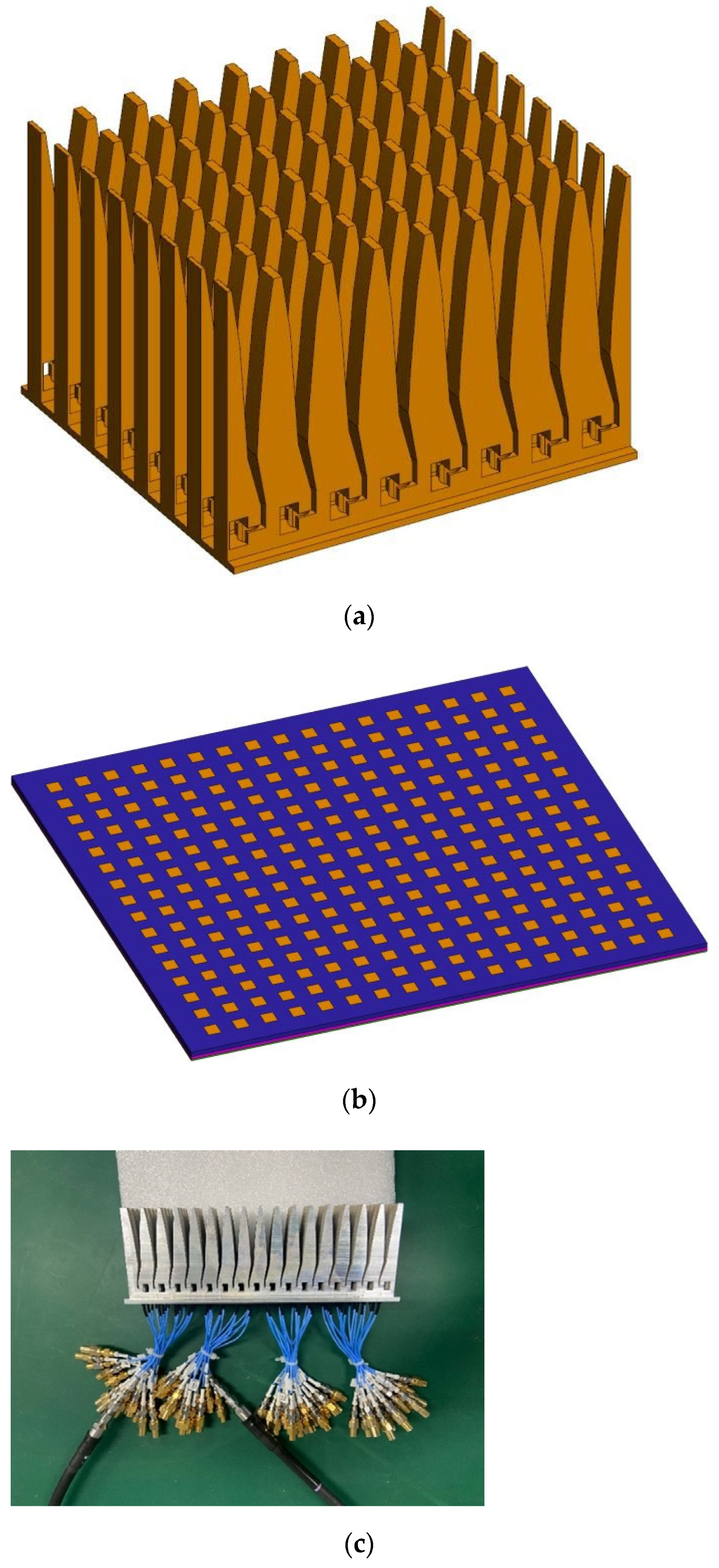
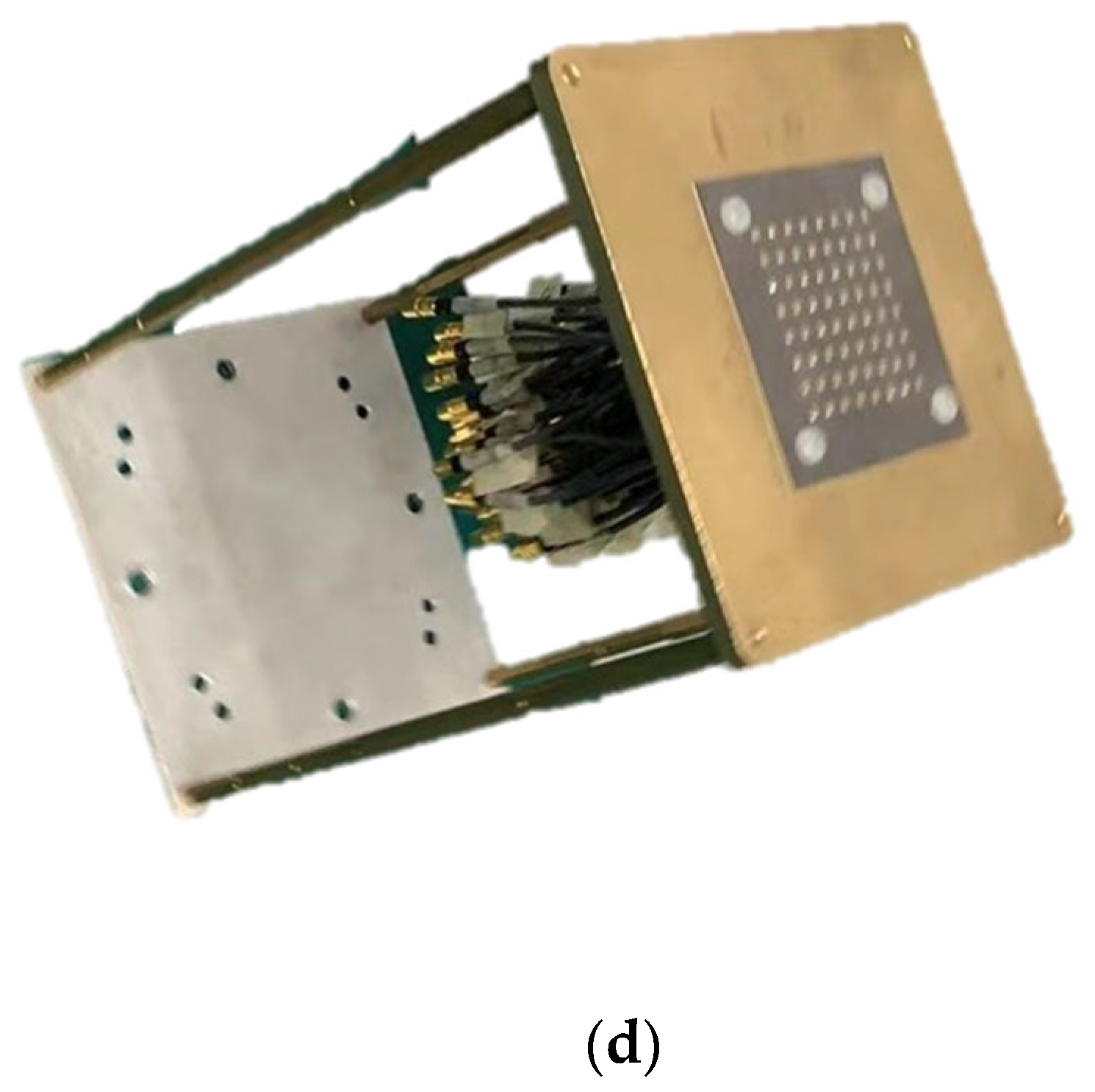
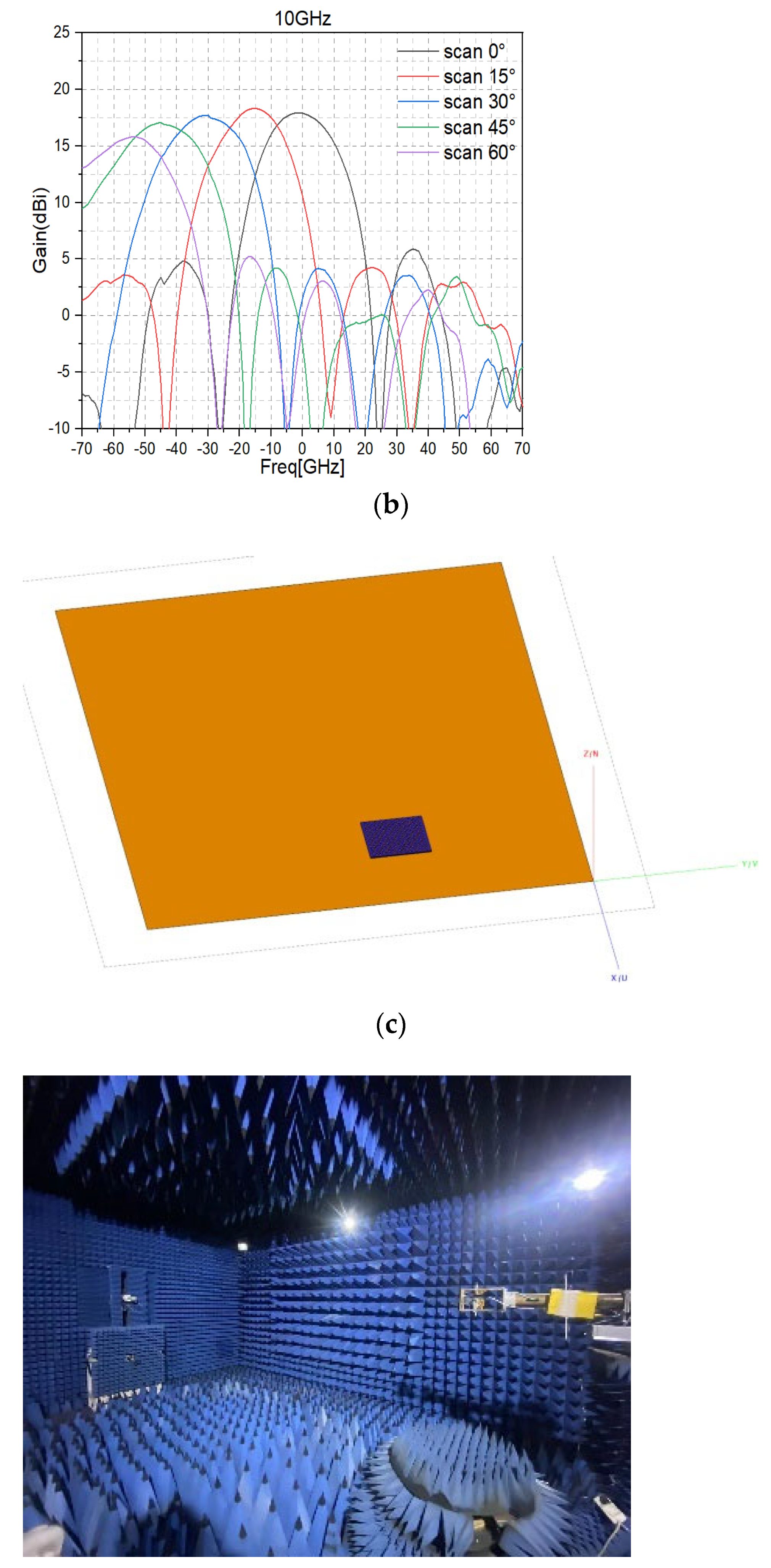
The antenna arrays are modeled as shown in Figure 3a,b, respectively, and the physical pictures and test statuses of the antenna arrays are given in Figure 3c,d, respectively. The electric field polarization directions of both arrays are consistent with the direction of the elastic axis (x-direction), and the two subarrays are arranged in the array as shown in Figure 4a,c. The E surface is the xoz surface and the H surface is the yoz surface. The practical test environment and the related results are also given in Figure 4b,d to prove the novelty of the proposed method.
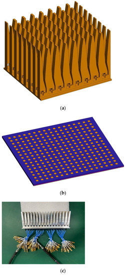

Figure 3.
Two antenna subarray structures. (a) 2–18 GHz ultra-broadband subarray structure. (b) 26–40 GHz microstrip antenna subarray structure. (c) 2–18 GHz Physical picture and test status of antenna array. (d) 26–40 GHz Physical picture and test status of antenna array.
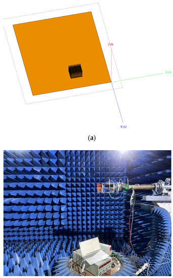
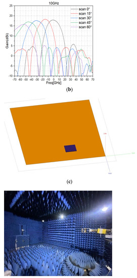
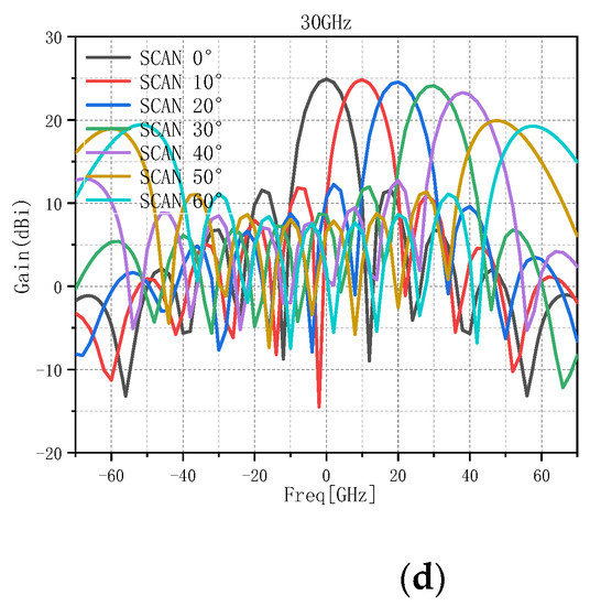
Figure 4.
Schematic diagram of the positions of the two antenna subarrays in the array. (a) 2–18 GHz of a subarray in the array. (b) Test environment and partial results of 2–18 GHz array. (c) Position of a subarray at 26–40 GHz in the array. (d) Test environment and partial results of 26–40 GHz array.
3.2. The Directional Map Synthesis of Ultra-Wideband Array
The improved simulated annealing (ISA) algorithm is used in the optimization process of determining the subarray position and the optimization process of deciding the subarray amplitude–phase distribution. The optimization results under three different optimization methods are compared.
- (1)
- The active direction map of the subarray without scanning capability (i.e., 0° scanning angle) is used to optimize the subarray position distribution, and then the direction map of the subarray without scanning capability in the direction of the H-plane side projection (0°) is optimized. We denote this optimization result by the symbol (0, 0).
- (2)
- The active directional map of the subarray without scanning capability (i.e., 0° scanning angle) is used to optimize the subarray position distribution. Then, the directional map of the subarray with scanning capability at 40 degrees in the H-plane (40°) is optimized. We denote this optimization result by the symbol (0, 40).
- (3)
- The subarray position distribution is optimized using the active directional map of the subarray with scanning capability (i.e., 40° scanning angle). Then the directional map of the subarray with scanning capability at 40 degrees in the H-plane (40°) is optimized. We denote this optimization result by the symbol (40, 40).
Improved simulated annealing (ISA) algorithms are used in the optimization process of determining the subarray position and the subarray amplitude–phase distribution for the three different optimization approaches. To compare the three different optimization approaches, the directional map of the ultra-wideband array at a typical scan angle at a 10 GHz operating frequency is selected for synthesis. Among them, the optimization constraint refers to the adjustable parameters in the ISA algorithm, which contains the following parameters: Gain in determining the subarray position indicates the expected decreased value of the overall gain of the antenna array after selecting the position (i.e., when the sparse array is laid out) relative to the full array distribution, and determining the subarray amplitude–phase distribution indicates the expected decrease value of the gain of the sparse antenna array after selecting the amplitude–phase relative to the equal amplitude and phase after the position is determined; on the mask set, SLL indicates the sub-flap level, that is, the decline in dB value relative to the peak radiation; GAP means that the allowed sparse array in the maximum radiation direction between the two masks is gain fluctuation value.
The valuation of gain in determining the subarray position is related to the effective area of the antenna array after indicating the selected status (i.e., when the array is sparsely laid out) and the full array, and the expected drop in overall gain of the antenna array can be estimated as . Because the full array gain and the subarray position gain are calculated by the scanning angles corresponding to the array direction map summation, determining gain in the subarray amplitude–phase distribution should try to take a smaller value so that the array determines the amplitude–phase after the final gain to the maximum, generally not less than −0.5 value. Here, considering that the expected drop in gain should be smaller than the theoretically calculated value (the absolute value is more significant), gain takes −3 dBi when determining the subarray position, and gain takes −0.5 dBi when determining the amplitude–phase distribution. Determine the value of the parameter in the process of subarray amplitude–phase distribution optimization:
3.2.1. Optimization Results for the (0, 0) Approach
The 25 subarray positions in yellow in Figure 5 are selected as the initial array distribution. The radiation direction map optimized by the position, the radiation direction map optimized by the amplitude–phase distribution, and the final subarray position and amplitude–phase distribution are shown in Figure 6, Figure 7, Figure 8 and Figure 9, respectively. The final array gain is 30.8444 dBi.
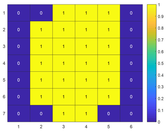
Figure 5.
Initial positions of the 25 subarrays (artificially selected).
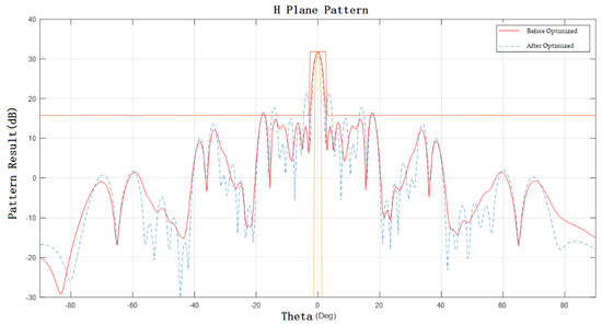
Figure 6.
Directional maps of E-plane and H-plane of the array after subarray position optimization at 0-degree scanning angle.
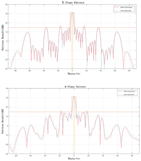
Figure 7.
The E-plane and H-plane orientations of the array after optimization of the subarray amplitude–phase distribution at 0-degree scan angle.

Figure 8.
Final position distribution and amplitude and phase distribution of the subarray at 0–degree scan angle.
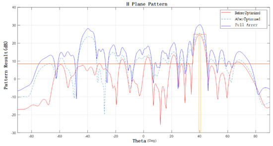
Figure 9.
H-plane orientation of the array after optimization of the subarray amplitude–phase distribution at 40-degree scan angle.
3.2.2. Optimization Results for the (0, 40) Approach
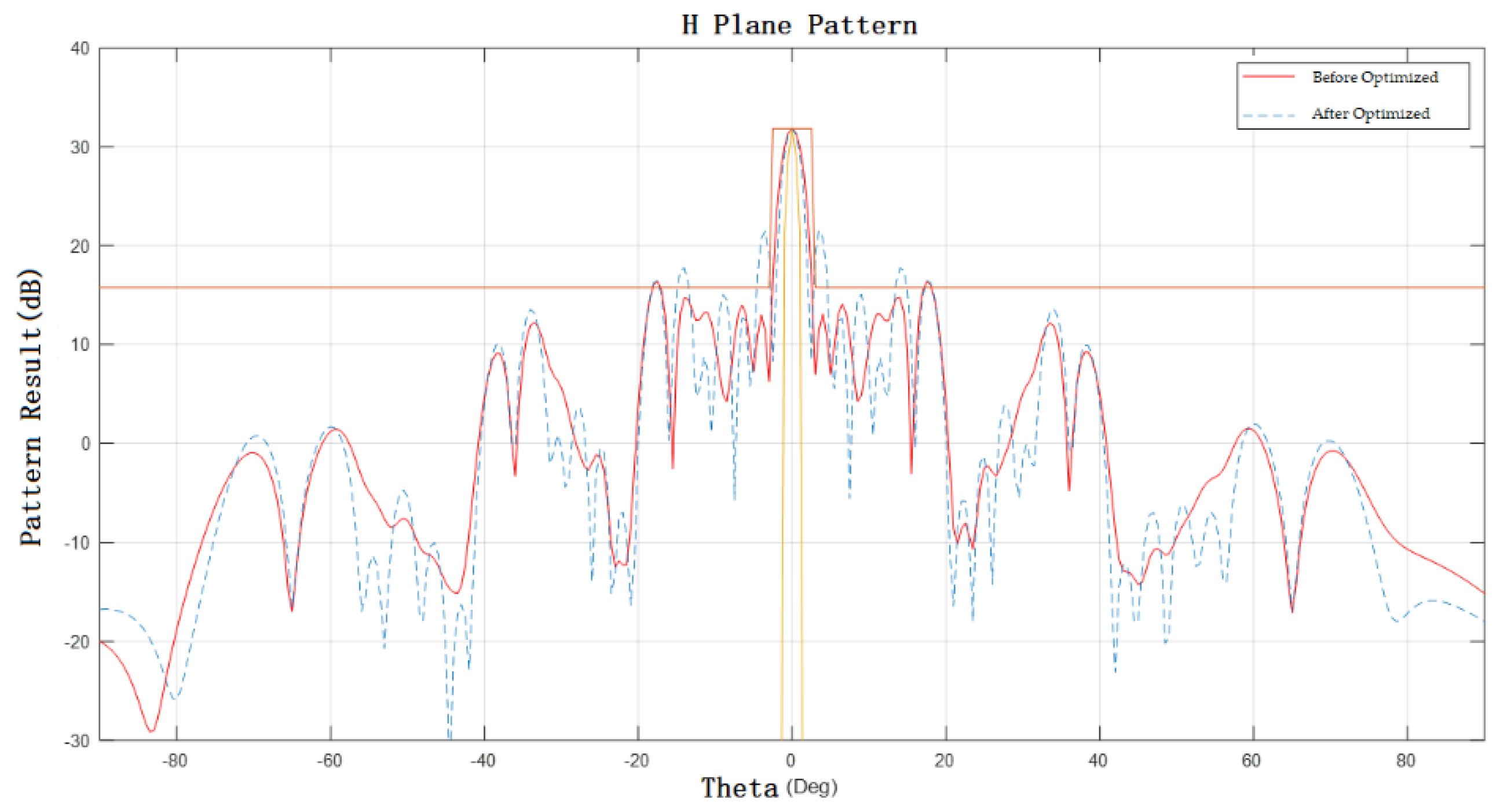
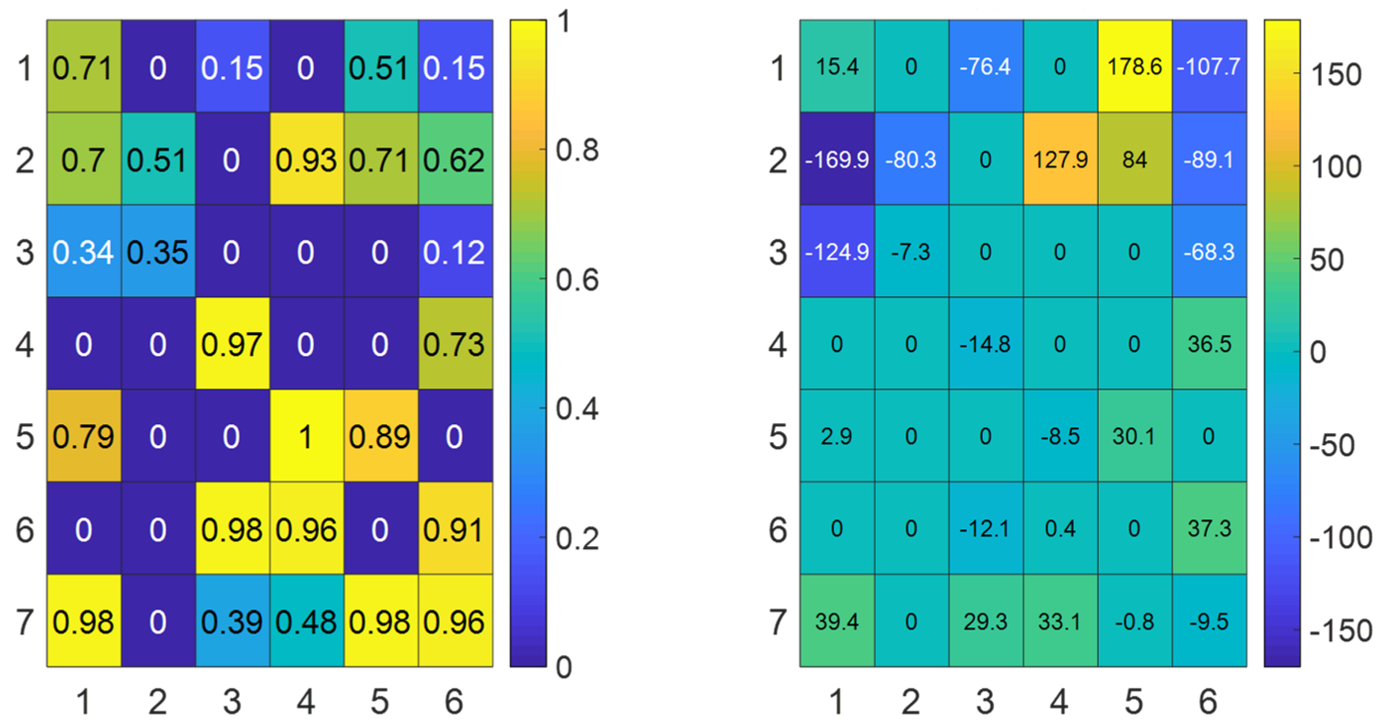
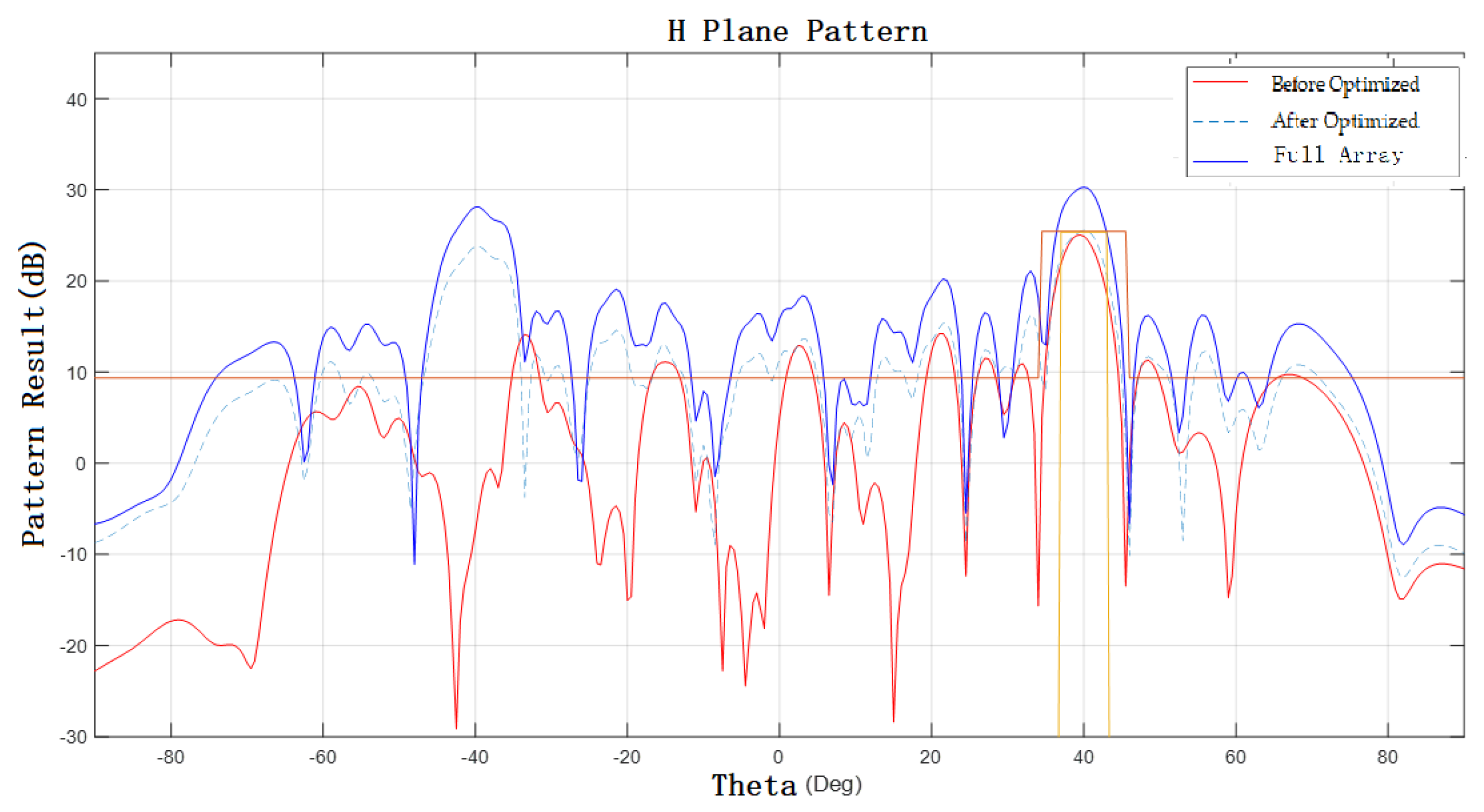
The subarray position is consistent with (a1), and the radiation direction map, the final subarray position, and the amplitude–phase distribution are shown in Figure 10 and Figure 11, respectively, after the amplitude–phase distribution optimization. The solid blue line in Figure 11 is the H-plane direction of the array when the whole array is in phase with equal amplitude; the dashed blue line is the H-plane direction of the array when the position is determined to be in phase with equal amplitude; and the solid red line is the final H-plane direction of the array after determining the amplitude distribution of the 25 subarray excitations. The final array gain is 24.5228 dBi.
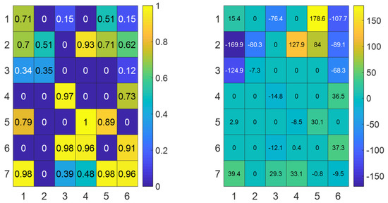
Figure 10.
Final position distribution and amplitude–phase distribution of the subarray at 40-degree scan angle.
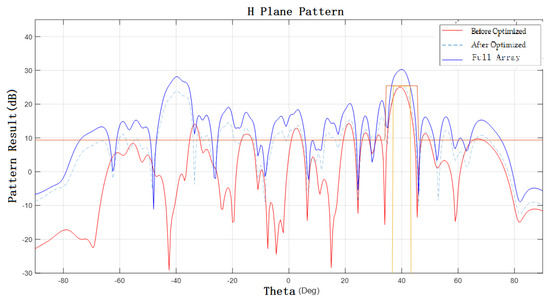
Figure 11.
H-plane orientation of the array after optimization of the subarray amplitude–phase distribution at 40-degree scan angle.
3.2.3. Optimization Results for the (40, 40) Approach
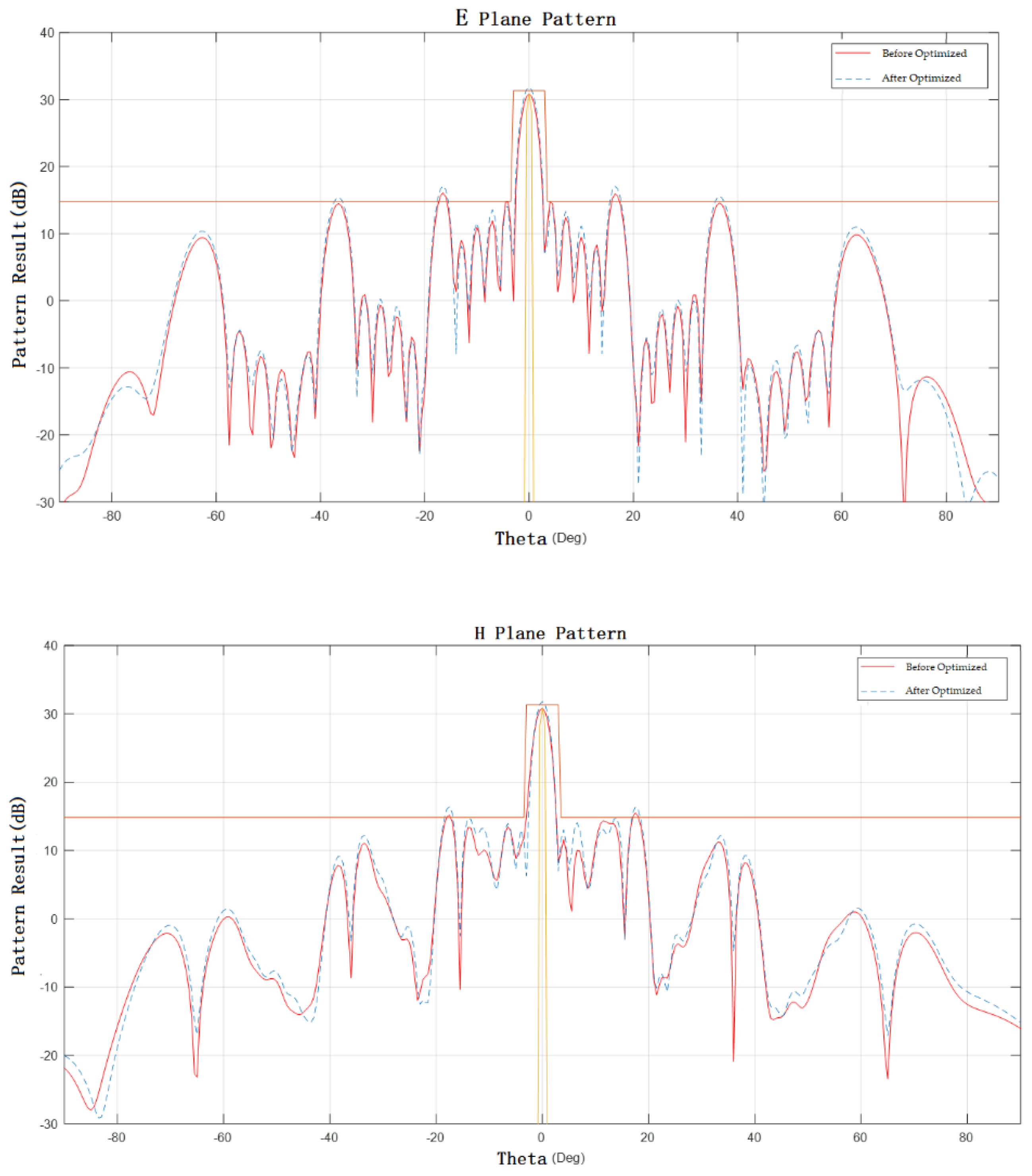
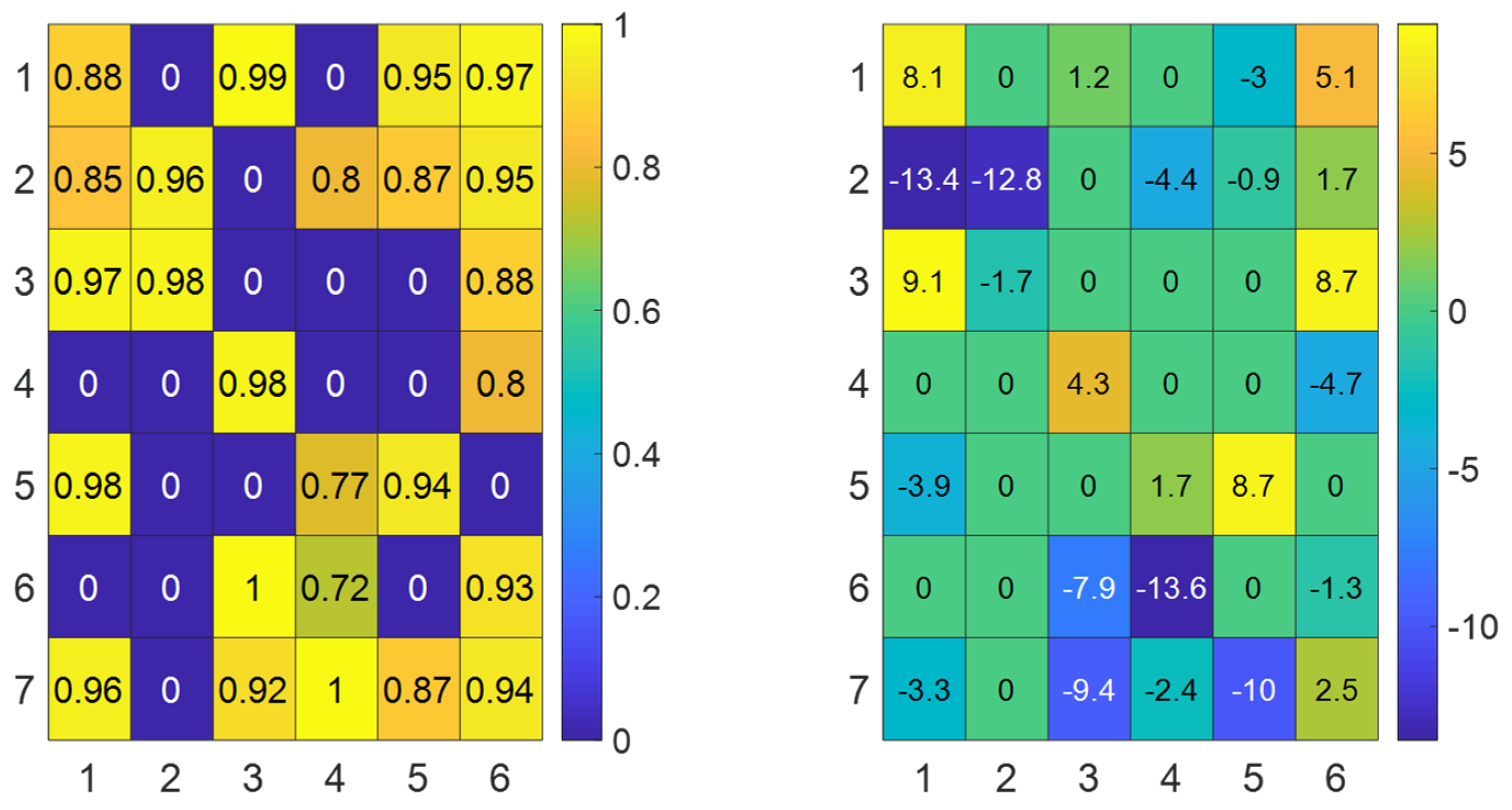
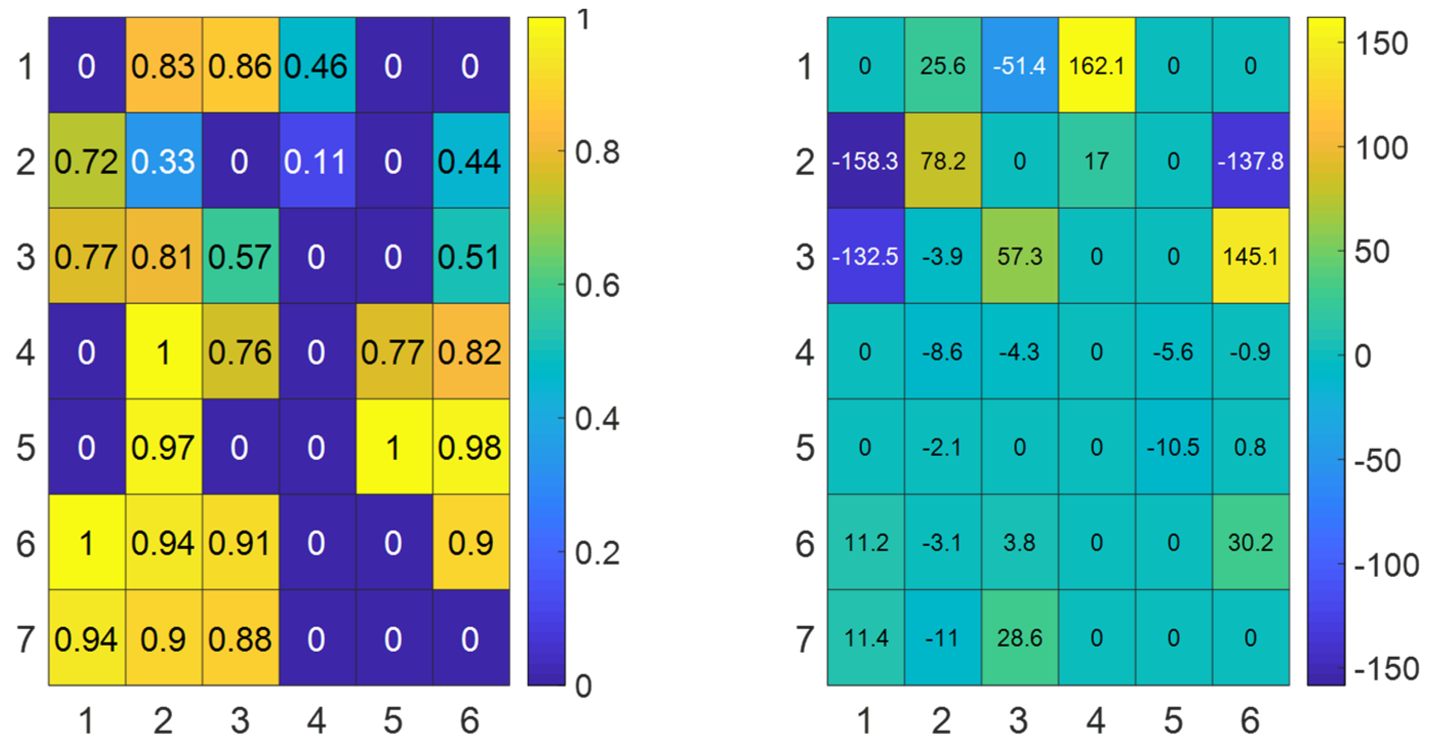
The subarray position is optimized by using the active direction map in the subarray array with a 40-degree scan angle, and the radiation direction map, the final subarray position, and the amplitude–phase distribution are shown in Figure 12 after the amplitude–phase distribution optimization. The absolute array gain is 25.05 dBi.
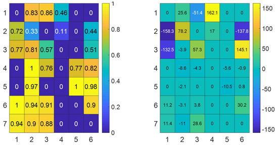
Figure 12.
Final position distribution and amplitude–phase distribution of the subarray at 40-degree scan angle.
Optimizing the amplitude–phase distribution with a scanning-capable subarray is better than optimizing the position without a scanning-capable subarray. In addition, optimizing the amplitude–phase with a scanning-capable subarray, i.e., the integrated result of the directional map of (40,40), is better than that of (0,40).
4. Conclusions
For the ultra-wideband array of 2–18 GHz, under the fixed frequency point, the amplitude and phase of the subarray feed that satisfies the performance index can be obtained by the optimization algorithm, firstly determining the subarray distribution position and then by the optimization algorithm. The current amplitude–phase optimization process uses an active directional map with subarray scanning capability, which can achieve good optimization results. This requires the subarray to have scanning capability in the H-plane, which is computationally intensive. If a non-scanning subarray directional map is used to optimize the directional map for any scanning angle, there is also a case of non-convergence of the optimization. Therefore, further optimization of the algorithm is required.
Author Contributions
Methodology, K.W.; software, Z.M. and H.X.; formal analysis, K.W. and Y.Z.; investigation, Y.Z.; resources, Y.D.; data curation, Y.L.; writing—original draft preparation, K.W.; writing—review and editing, K.W.; visualization, M.H.; supervision, Y.Z.; project administration, Y.Z.; funding acquisition, Y.Z. All authors have read and agreed to the published version of the manuscript.
Funding
This paper is funded by the Scientific and Technological Innovation Foundation of Foshan, USTB (BK22BF002).
Data Availability Statement
Data sharing not applicable.
Conflicts of Interest
The authors declare no conflict of interest.
References
- Shi, D.; Lian, C.; Cui, K.; Chen, Y.; Liu, X. An Intelligent Antenna Synthesis Method Based on Machine Learning. IEEE Trans. Antennas Propag. 2022, 70, 4965–4976. [Google Scholar] [CrossRef]
- Guo, Y.J.; Ziolkowski, R.W. A Perspective of Antennas for 5G and 6G. In Advanced Antenna Array Engineering for 6G and beyond Wireless Communications; IEEE: Piscataway, NJ, USA, 2022; pp. 1–22. [Google Scholar]
- Zhou, H.; Geng, J.; Wang, K.; He, C.; Liang, X.; Jin, R. Dual-Polarized Wide-Angle Scanning Linear Phased Array Antenna Design With High Polarization Isolation. IEEE Antennas Wirel. Propag. Lett. 2022. [Google Scholar] [CrossRef]
- Rafique, U.; Dalal, P.; Abbas, S.M.; Khan, S. Phased Array Antenna for Millimeter-Wave 5G Mobile Phone Applications. In Proceedings of the 2022 IEEE Wireless Antenna and Microwave Symposium (WAMS), Rourkela, India, 5–8 June 2022; pp. 1–4. [Google Scholar]
- Chatterjee, P.; Nanzer, J.A. Using platform motion for improved spatial filtering in distributed antenna arrays. In Proceedings of the 2018 IEEE Radio and Wireless Symposium (RWS), Anaheim, CA, USA, 15–18 January 2018; pp. 253–255. [Google Scholar]
- Pavel, S.R.; Zhang, Y.D. Neural Network-Based Compression Framework for DOA Estimation Exploiting Distributed Array. In Proceedings of the ICASSP 2022—2022 IEEE International Conference on Acoustics, Speech and Signal Processing (ICASSP), Singapore, 22–27 May 2022; pp. 4943–4947. [Google Scholar]
- Xiao, Q.; Yang, S.; Bao, H.; Chen, Y.; Qu, S. A wideband dual-polarized conformal phased array based on tightly coupled dipoles. In Proceedings of the 2017 Sixth Asia-Pacific Conference on Antennas and Propagation (APCAP), Xi’an, China, 16–19 October 2017; pp. 1–3. [Google Scholar]
- Infante, L.; Mosca, S.; Angelilli, M. Conformal Phased Array Calibration Based on Orthogonal Coding: Theory and Experimental Validation. In Proceedings of the 2019 IEEE International Symposium on Phased Array System & Technology (PAST), Waltham, MA, USA, 15–18 October 2019; pp. 1–5. [Google Scholar]
- Wang, Z.; Zhang, G.; Yin, Y.; Wu, J. Design of a Dual-Band High-Gain Antenna Array for WLAN and WiMAX Base Station. IEEE Antennas Wirel. Propag. Lett. 2014, 13, 1721–1724. [Google Scholar] [CrossRef]


Publisher’s Note: MDPI stays neutral with regard to jurisdictional claims in published maps and institutional affiliations. |
© 2022 by the authors. Licensee MDPI, Basel, Switzerland. This article is an open access article distributed under the terms and conditions of the Creative Commons Attribution (CC BY) license (https://creativecommons.org/licenses/by/4.0/).