Very Simple System for Walking-Speed Measurement in Geriatric Patients

Abstract

Walking speed in geriatric patients is an important index for inferring the patient’s state of health and estimating the success rate of some surgical procedures. Although different solutions for monitoring the gait of a subject exist in scientific literature and on the market, there is a need for a system that is very simple, especially to wear, considering that elderly subjects often have movement difficulties. For this reason, we investigated the possibility of using a standard miniaturized wireless microphone, that can be easily attached to patients’ clothes by means of a clip, as the sole sensing device to be worn by the test subject. A transceiver, a sound card and a PC complete the system, which turns out to be quite simple to be set up and use, thanks to a proper graphic user interface that controls its entire operation. The system essentially tracks the position of the test subject over time by measuring the propagation times of repeated sound pulses from the speaker to the microphone. To avoid hearing discomfort, the frequency of the pulses is chosen at the higher end of the audio spectrum, so that they are essentially undetectable by adults. The measurement range is in excess of 6 m, that is sufficient for the standard 4 m walking-speed test. Tests performed in a laboratory environment have confirmed the effectiveness of the approach we propose.

1. Introduction

The evaluation of functional status is a key part of a comprehensive geriatric assessment and for this purpose the 4 m gait-speed test at individual’s usual pace is a commonly used tool both in clinical practice and in research [1].

Gait speed is not merely an expression of functional status; indeed, it serves as a significant predictor of cognitive impairment, in the context of aging trajectories toward frailty and disability [2].

Therefore, gait speed may be considered a new “vital sign” (in addition to other well-known signs, such as blood pressure or heartbeat), and it represents a marker of health status [3,4] and a potential predictor of mortality and disability in older men and women [5,6,7,8,9,10,11].

The concordance of manual or instrumental (accelerometer) assessment of 4 m walking speed is not optimal and manual measures might lead to misclassification of a substantial number of subjects [12]. To avoid incorrect medical diagnosis, it would be desirable to use electronic measuring systems. However, for the 4 m gait-speed test there is no dedicated system and usually the walking-speed measurement system integrated in gait-analysis [13,14] systems is used. However, gait-analysis systems are quite complex since they aim to estimate other parameters as well [15,16,17,18,19,20,21,22,23,24,25,26,27].

Among the methods used to perform gait analysis, a few methods are laboratory-based and employ optometric systems or force sensors [13,18,28,29,30]. However, these systems are quite expensive and require measurement set-ups that are time-consuming and too complex to implement for medical staff. Moreover, they also require post-processing operations that are usually manual and not automatic and are therefore suitable for laboratory environments but not for routine use in clinics [31,32,33]. Thanks to the advances made in the field of embedded systems [34,35] and sensors [36,37,38,39,40] the implementation of portable or wearable monitoring systems has become quite widespread. Usually, such systems are based on wearable or body-fixed sensors (BFSs) together with miniaturized inertial measurement units (IMUs), that consist of accelerometers, gyroscopes and, in some cases, magnetometers [41,42].

Although these systems are certainly effective and much more practical to use than conventional laboratory methods, they often require the BFSs and IMUs to be attached to different parts of the body or to be worn with special harnesses. These are sacrifices that can be endured when a gait-analysis test must be performed, but when only a 4 m walking-speed test has to be performed these solutions might be too complex for the medical professional and too invasive for the patient. Indeed, especially in the case of elderly patients with movement difficulties, the availability of a system that is easy to put on and quick to use becomes perhaps the most important requirement to be satisfied (in addition, of course, to sufficient accuracy in the measurements). Less invasive systems based on LiDAR (light detection and ranging) that can certainly reduce the level of stress suffered by the test subjects have been recently proposed [43,44]. One such system appears to be particularly interesting as a candidate for replacing the manually assessed 4 m walking-speed test, since it is based on a simple LiDAR sensor and the position of the test subject can be measured passively, that is with no sensor being worn by the patient [44]. On the other hand, the system still requires a piece of dedicated hardware (a microcontroller unit driving the LiDAR sensor) that, while not complex in principle, cannot be regarded, at present, as an off-the-shelf component.

Starting from these considerations, in this paper we present a system for measuring the walking speed whose structure is entirely based on easily available off-the-shelf components and that requires that the elderly patient only wears a standard miniaturized wireless clip microphone. The rest of the system is composed of a wireless microphone receiver, a PC sound board for signal generation and acquisition, a speaker system for sound generation and a personal computer for signal elaboration that runs a dedicated software developed for this specific application. Since the system is based on quite standard equipment and the dedicated software is entirely based on public-domain libraries, we trust that it can be easily reproduced and employed with minimum effort even by medical professionals lacking an advanced background in ICT.

2. Materials and Methods

Our approach in designing a new system for walking-speed measurement in geriatric patients was that of searching for a set-up that did not require the development of dedicated hardware and that was simple enough in its structure to allow any interested medical professional to easily reproduce it with minimal investment in terms of cost and effort. Besides quite standard hardware components, the system relies on dedicated software that is made freely available by the authors.

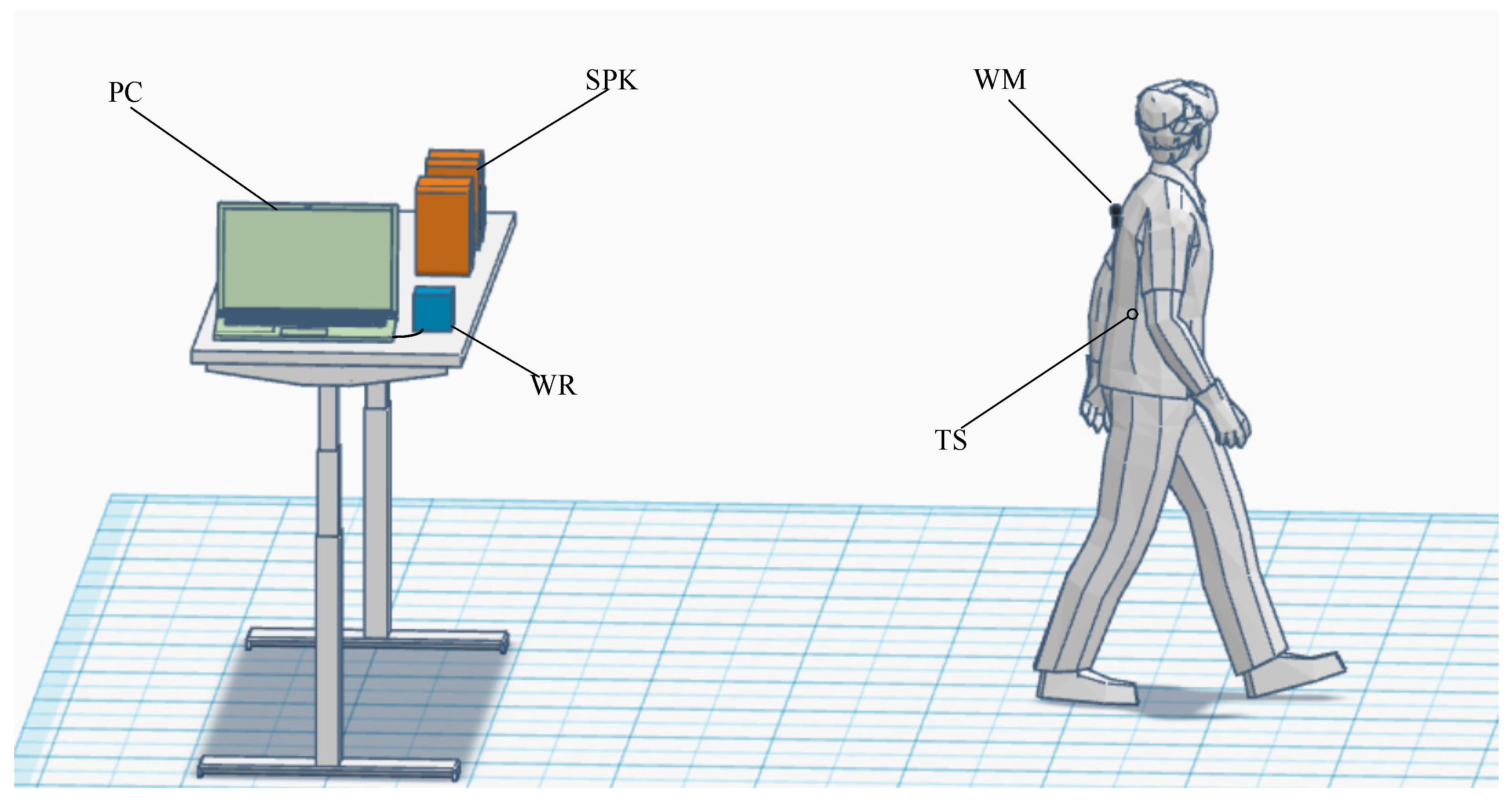
The principle of operation of the system can be summarized as follows (Figure 1):

• A PC, by means of a sound card, generates sound pulses that are diffused by a speaker (SPK in Figure 1) into the environment toward the test subject (TS);
• The test subject wears a compact wireless microphone (WM) that detects the pulses and sends the audio signal being received back to the wireless microphone receiver (WR), whose audio output is connected to the input of the sound board used for generating the pulse in the first place;
• The distance traveled by each pulse, while the patient walks, is obtained by multiplying the speed of sound by the time delay between the received and the corresponding transmitted pulse (the propagation time of radio waves on the way back is negligible);
• The position vs. time for many successive pulses is recorded so that the average speed of the patient (or even more complex cinematic indicators) can be easily extracted.

While PC soundboards can be capable of sampling frequencies up to 192 kHz and can be used in measurement applications above 20 kHz [45], other standard audio hardware (microphone and low-end PC speakers) typically cannot handle frequencies in excess of 20 kHz. On the other hand, producing sound pulses that can be sensed by the patient and by the operator would result in a quite uncomfortable environment. Fortunately, at least in the case of this application in which all persons involved are either mature or elderly people, the human ear becomes quite insensitive to sound in the frequency range between 16 kHz and 20 kHz as age increases [46,47]. As long as the frequency content of the generated pulses falls within this frequency range, the pulses cannot be heard by either the patient or the medial operators in the testing environment. For an efficient use of this bandwidth, we chose to generate pulses with a (selectable) carrier frequency in the range 17–19 kHz with a Gaussian envelope. Note that the operator still retains the ability to set a carrier frequency at lower frequency and this feature can be quite useful in order to produce easily audible “beeps” during the initial system set-up.

Given a Gaussian signal in the form:

$$s\left(t\right)=A{e}^{-\frac{t^2}{2{\tau }^2}}$$

(1)

its Fourier transform S(f) can be written in the form:

$$S\left(f\right)=ℱ\left[s\left(t\right)\right]=A\tau \sqrt{2\pi } e^{-\frac{f^2}{2f_{\tau }^2} } ; f_{\tau }=\frac{1}{2\pi \tau }$$

(2)

Plots of s(t) and S(f) are reported in Figure 2 to evidence that while they are, in principle, not limited in time and in frequency, respectively, an effective pulse duration t_D = 4τ and a corresponding overall bandwidth occupancy B = 4f_τ = 1/t_D can be identified. When the pulse s(t) is used to modulate a carrier at frequency f_C, S(f), apart for a scale factor, is translated across f_C.

In selecting the pulse duration for our application, we must account for a number of competing factors. While a very short pulse would be better suited for target localization, the fact that the available bandwidth that can be used is 4 kHz (from 16 kHz up to 20 kHz assuming f_C = 18 kHz) means that the pulse duration must be larger than 640 μs (τ > 160 μs) that, with the speed of sound being about 346 m/s at 25 °C, corresponds to an equivalent distance in space of about 22 cm. There are, however, reasons for extending the duration of the pulse even more. In the first place, even if consumer-grade microphones and speakers can have a non-negligible response above 16 kHz, it has to be assumed that at frequencies close to the cut-off, significant phase roll-off occurs with the risk of introducing linear distortion that can interfere with the target location. Clearly, the effect of such distortion can be limited if the fractional bandwidth of the signal (that is of the pulse) is reduced. Moreover, measurements in this specific application will occur in a clinic with the microphone picking up noise and possibly the very voices of the medical staff and of the patient during the walk. Having a smaller bandwidth for the signal (i.e., a longer duration for the pulse) facilitates the rejection of disturbances during elaboration. In actual experiments, pulse duration 4τ was close to 1.9 ms, for a corresponding effective bandwidth of about 1.3 kHz.

The ability to generate and acquire pulses with the required specification is well within the capabilities of most audio subsystems integrated with modern personal computer. However, in order to provide a clear reference for those researchers interested in experimenting with the approach discussed in this paper, we resorted to the USB sound board Behringer U-PHORIA UMC202HD [48] that can operate with a sampling frequency up to 192 kHz and uses 24 bits analog digital (AD) and digital analog (DA) front ends. More importantly, the selected USB audio board comes with its own ASIO driver that is useful in reducing latency in audio elaboration, as we shall discuss momentarily. As far as the wireless microphone is concerned, we have selected a miniaturized RODE system [49] completed with a clip microphone [50]. In this way, the tiny transceiver can be easily placed in a pocket of the patient, with the clip microphone “clipped” on the clothes of the patient. The selection of the speakers is, in a way, more problematic. Typically, limitations in the frequency response of non-professional PC speakers are toward the low frequency range. In our case, however, it can be argued that the smaller the size of the speakers, the better, since a smaller speaker is expected to better respond to high audio frequencies, provided that there are no bandwidth limitations in the electronics. Unfortunately, technical documentation on consumer speakers is particularly vague on this point. Experiments on a number of low-end PC speakers (price range below EUR 100) revealed that in almost all cases non-linear compression effects are present. These cause non-linear distortions on the transmitted sound pulse at relatively low power levels. Much better results have been obtained using mid-range compact HiFi systems and indeed, in the experiments presented in this paper we employed a Philips BTM177 system for sound amplification [51]. Note, however, that, if required, the speaker system is possibly one of the easiest pieces of instrumentation to customize. Indeed, tweeter loudspeakers for HiFi applications with a frequency response exceeding 20 kHz are easily available on the market.

For development of the system software, we resorted to the PortAudio public-domain library for interfacing with the audio board [52]. A simple graphical interface for system-level operation by medical personnel was developed in QT [53].

The detailed implementation of the signal generation and elaboration chain is illustrated in Figure 3. The vertical dashed line in Figure 3 marks the separation between the signal-elaboration domain (to the left of the line) from the physical world (to the right of the line). In a way, the vertical line, together with the delays Δt₁ and Δt₂, represents the action of the audio board that connects the numerical elaboration performed by the personal computer with the electrical signals in the real world (the signal toward the speakers and the signal coming from the radio receiver). The delays Δt₁ and Δt₂ represent the latency introduced in the DA path and in the AD path, respectively, by the audio board. These delays, for a given configuration of the audio board, are constant and, since we are interested in measuring position changes, are, in principle, uninfluential in the speed estimation process. However, typical latencies for audio boards can be large with respect to the propagation time of the sound pulse from the speakers to the microphone and can limit the pulse repetition frequency that can be obtained. ASIO-compliant audio boards, as in the one selected for this design, are to be preferred in this respect since they allow to minimize latency.

When dealing with a moving target (the patient walking), the Doppler effect is present and one must also take into consideration possible errors arising from it. In discussing the operation of the system, we will assume perfect mono-dimensionality, that is, everything occurs along the x axis. Let us start by discussing the following hypothetical scenario: the base station is in a fixed position x_B and emits a signal T(t); the target at the reference time t = 0 is located at position x_T0 and moves with a constant speed v_T along the x axis. In this situation we have, for the position x_T of the target and the distance d_TB = x_T − x_B between the target and the base station:

$$\begin{array}{c}{x}_T\left(t\right)=x_{T0}+v_{T}t\\ d_{TB}\left(t\right)=x_{T0}-x_B+v_{T}t=d_{TB0}+v_{T}t\end{array}$$

(3)

We will assume the condition d_TB > 0 at all the times of interest.

What reaches the target at time t must have left the base station a time interval in the past Δt equal to the time needed to cover the distance d_TB(t) with the propagation speed v_p, that is:

$$∆t\left(t\right)=\frac{d_{TB}\left(t\right)}{v_p}=∆t_0+\alpha t ; ∆t_0=\frac{d_{TB0}}{v_p} ; \alpha =\frac{v_T}{v_p}$$

(4)

Therefore, we have, for the signal R(t) received by the target:

$$R\left(t\right)=\beta T\left(t-∆t\left(t\right)\right)=\beta T\left[\left(1-\alpha \right)t-∆t_0\right]$$

(5)

where β is an attenuation factor that depends on the distance and, hence, on t. However, we can assume β to be essentially constant within the duration of a single pulse. If a very short pulse T_SP could be generated by the base station at t = t_p, that is:

$$T_{SP}\left(t\right)=A_{SP}\delta \left(t-t_p\right)$$

(6)

According to Equation (5), we will have for the signal R_SP received by the target:

$$R_{SP}\left(t\right)=\beta \delta \left[\left(1-\alpha \right)t-∆t_0-t_p\right]$$

(7)

Therefore, the pulse will reach the target at the time t_r for which the argument of the delta function in Equation (7) is zero, that is with a propagation delay Δt_p given by:

$$∆t_p=t_r-t_p=\frac{1}{1-\alpha }∆t_0+\frac{\alpha }{1-\alpha }{t}_p$$

(8)

If we can measure the propagation delay, from Equation (6) we obtain, using the propagation speed v_p, the distance of the target from the base station at the time t_r = t_p + Δt_p.

The fact is that in the set-up we are working in, it is not possible to generate extremely short pulses because of the limitation in the bandwidth of the several devices involved in the measurement chain (audio boards, speakers, microphone). We will resort, therefore, to a different approach, as discussed before.

Let us assume the transmitted signal T(t) to be a sinusoidal signal modulated by a Gaussian pulses g_T(t) with

$$g_T\left(t\right)=A_T{e}^{-\frac{t^2}{2{\tau }^2}}$$

(9)

Let us take into consideration the case of a single Gaussian pulse centered at t = t_p. We have, for the transmitted signal T(t):

$$T\left(t\right)=g_T\left(t-t_p\right)\cos \left({\omega }_{C}t\right)=A_T{e}^{-a\frac{{\left(t-t_P\right)}^2}{2{\tau }^2}}\cos \left({\omega }_{C}t\right)$$

(10)

The signal detected at the target is, therefore:

$$R\left(t\right)=\beta g_T\left(\left[\left(1-\alpha \right)t-∆t_0-t_p\right]\right)\cos \left\{{\omega }_C\left[\left(1-\alpha \right)t-∆t_0\right]\right\}$$

(11)

In order to simplify the notation, let us define:

$$g_R\left(t\right)=\beta g_T\left(\left[\left(1-\alpha \right)t-∆t_0-t_p\right]\right)$$

(12)

At the input of the LPF Figure 3 we have:

$$R\left(t\right)e^{j{\mathsf{\omega }}_{C}t}=I_{mix}\left(t\right)+j{Q}_{mix}\left(t\right)$$

(13)

With

$$\begin{array}{ccc}{I}_{mix}\left(t\right)& =& g_R\left(t\right) cos\left\{{\mathsf{\omega }}_C\right[\left(1-\mathsf{\alpha }\right)t-\mathsf{\Delta }{t}_0\} cos\left({\mathsf{\omega }}_{C}t\right)=\\ & =& \frac{g_R\left(t\right)}{2}\left(cos\left\{{\mathsf{\omega }}_C\right[\left(2-\mathsf{\alpha }\right)t-\mathsf{\Delta }{t}_0\}+cos\{{\mathsf{\omega }}_C[\alpha t+\mathsf{\Delta }{t}_0]\} \right)\end{array}$$

(14)

$$\begin{array}{ccc}{Q}_{mix}\left(t\right)& =& g_R\left(t\right) cos\left\{{\mathsf{\omega }}_C\right[\left(1-\mathsf{\alpha }\right)t-\mathsf{\Delta }{t}_0\} sin\left({\mathsf{\omega }}_{C}t\right)=\\ & =& \frac{g_R\left(t\right)}{2}\left(sin\left\{{\mathsf{\omega }}_C\right[\left(2-\mathsf{\alpha }\right)t-\mathsf{\Delta }{t}_0\}+sin\{{\mathsf{\omega }}_C[\alpha t+\mathsf{\Delta }{t}_0\} \right)\end{array}$$

(15)

With the assumption of α << 1 and effective bandwidth of the Gaussian pulse much smaller than ω_C, the LPF can be designed to reject the high-frequency components in I_mix and Q_mix, so that the complex signal m(t) at the output of the LPF becomes:

$$m\left(t\right)=\frac{g_R\left(t\right)}{2}\left\{cos\left[{\omega }_C\left(\alpha t+\mathsf{\Delta }{t}_0\right)\right]+jsin\left[{\omega }_C\left(\alpha t+\mathsf{\Delta }{t}_0\right)\right]\right\}=\frac{g_R\left(t\right)}{2}{e}^{j{\omega }_C\left(\alpha t+\mathsf{\Delta }{t}_0\right)}$$

(16)

We have therefore:

$$\left|m\left(t\right)\right|=\frac{g_R\left(t\right)}{2}=\frac{\beta }{2}{g}_T\left(\left[\left(1-\alpha \right)t-∆t_0-t_p\right]\right)$$

(17)

By monitoring |m(t)| at the output of the low-pass filter, we can detect the time instant t_RMAX at which the envelope |m(t)| reaches its maximum, that is the time at which the argument of the function g_T in Equation (17) is zero. Please note that this condition is the same as the one used to obtain t_r and the propagation delay in Equation (8). Since we know t_p and we can experimentally detect t_rMAX, we can obtain the distance between the target and the base station ad time t_rMAX as:

$$d_{TB}\left(t_{RMAX}\right)=\frac{t_{RMAX}-t_p}{v_p}$$

(18)

Let us now observe that for Equation (18) to hold independently of the fact that the target is stationary or is moving it is not really necessary to assume a constant velocity at all times—the same solution is obtained with the much less demanding assumption of the target moving with constant speed only within the time interval in which it interacts with the pulse coming from the base station, that is the effective duration of the Gaussian pulse being received (in the order of 2 ms in our application). Since this is a quite reasonable assumption in the framework of our experiment, the result in Equation (18) holds for each single pulse.

In the actual implementation of the system, in order to facilitate the detection of the maximum and to improve noise rejection, the low-pass filter is implemented as a matched filter with an impulse response that, apart for a constant factor, coincides with the modulating Gaussian pulse in the transmitter chain.

A problem to be addressed is the possible presence of multiple pulses at the input of the system caused by the fact that, as well as along the direct path, the transmitted pulse can reach the microphone after being reflected by walls or other obstacles in the environment in which the measurement of the walk speed is performed. The fact that the walk-speed measurement is performed in a controlled environment can greatly help in setting up simple countermeasures, such as the use of drapery or folding screens (already available in a medical clinic), to reduce the multipath effect that in the frequency range we are interested in (16 to 20 kHz). Note that a pulse duration of 1.9 ms, as used in our experiments, corresponds to a physical length of about 66 cm. This means that, provided the room in which the measurement is performed is not too small, echoes coming from reflection on the walls are well separated in time from the pulse due to the direct path. This observation is used in the software that has been developed, in which a tracking algorithm ensures that even large peaks that appear during the patient tracking are ignored if they fall outside what is the reasonable expected change of position in time. In particular, at the beginning of the measurement, with the patient still and in a predefined position, the software locks on the peak corresponding to the direct path and maintains the lock during the entire measurement process.

Another relevant aspect that needs to be addressed is the fact that the speed of sound changes with temperature. Around room temperature the change is in the order of 0.61 (m/s)/°C, or, in terms of relative change, 0.18%/°C. Once again, the fact that we perform the measurements in a controlled environment helps in reducing the error coming from an incorrect estimation of the room temperature. Indeed, we expect the temperature in a medical clinic to be known and well regulated. At the present stage of development, the software assumes a default room temperature of 25 °C, but the operator can set the correct value of the ambient temperature at the beginning of the test. Note, however that with an error in the temperature value as high as 5 °C, the resulting error in the estimation of the speed of sound, and, consequently, in the walk speed of the patient, remains below 1%. The fact that the value of the room temperature has to be typed in by the operator is a choice that we have made to keep the system as simple as possible. Clearly, an automatic assessment of the temperature can be easily obtained by integrating a remote readable ambient thermometer as part of the system.

3. Results

A first set of tests was aimed at assessing the performance of the system with the microphone located at a known distance from the target. We wanted to evaluate the resolution and repeatability of distance estimation both in a silent environment and in more realistic situations in which ambient noise is present at significant levels as can be the case in a clinic. All experiments were performed with a carrier frequency f_C = 18 kHz and a time constant for the Gaussian pulse τ = 640 μs (pulse duration 4τ = 1.9 ms). The sampling frequency f_S of the audio board was set to the standard rate of 96 kHz. The overall delay Δt₁ + Δt₂ in the chosen operation conditions was about 10 ms (Figure 3), and assuming a maximum range of 10 m (propagation time of about 30 ms), a maximum pulse repetition frequency (PRF) of about 25 Hz. In our experiments the PRF was set to 15 Hz. In a first experiment the microphone was set at a distance of 2 m from the speaker in a silent environment. The pulse signal received from the microphone (R(t) in Figure 3) is reported in the upper graph in Figure 4a. The output of the correlator (|m(t)| in Figure 3) is reported in the bottom graph in Figure 4a. The time delay from the received pulse and the output of the correlator in Figure 4a depends on the way in which the numerical computation of the output of the correlator is performed. This time delay, as well as the time delay Δt₁ + Δt₂ is not relevant since we aim to measure relative changes in the position of the target. When the target moves from position x₁ to position x₂, the position difference x₂ − x₁ is obtained starting from the observation of the displacement in time of the maxima of the correlator output. All operations, including the calculation of the correlator output, are performed in the discrete time domain with a quantization time equal to the inverse of the audio board sampling frequency, that is Δt = 1/f_S. In our operating condition (f_S = 96 kHz) the quantization time Δt = 10.42 μs. This means that we obtained a resolution in the estimation of the position of the maximum from the sampled correlation output of about 3.6 mm. While this resolution can be considered sufficient for our application, we implemented a different approach for the estimation of the position of the maximum that, in addition to providing more resolution, was more robust in terms of noise and artefact rejection. In our approach we used the position of the maximum as obtained from the raw sampled data at the output of the correlator as an initial guess. A set of samples across the position of the estimated maximum corresponding to a duration of about 2τ was selected (as in Figure 4a, bottom graph) and are fitted against a parabolic approximation of the correlator output close to the maximum. The position of the vertex of the fitting parabola was taken as the position of the maximum. In order to verify the behavior of the system in the presence of ambient noise, we played back a recording of several people talking together and adjusted the level of the reproduction so that the peak-to-peak signal picked up by the microphone was comparable to the peak-to-peak amplitude of the pulse received in a silent environment.

A sample of the recorded signal in this condition is reported in the top graph in Figure 4b, where we have the ambient noise and the pulse superimposed. The output of the correlator in this situation is reported in the bottom graph in Figure 4b and it can be verified that no significant change in the shape of the curve close to the maximum can be observed. A second experiment was performed in order to evaluate the accuracy with which the system can detect the position of the target over repeated measurement in silence and in the presence of noise. In this second experiment the microphone was located at 4 m from the speaker. The peak-to-peak amplitude of the received pulse was reduced to about 80 mV pp, as shown in the top graph in Figure 5a. The deviation of the estimated position over a time of about 4 min (for a total of about 3600 pulses) was recorded and the result is shown in the bottom graph in Figure 5a. As can be seen, the absolute estimation error always remained well below 5 mm, and the standard deviation in the recorded error was about 1.48 mm over a distance of 4 m. Since these performances were obtained in a silent environment, they have to be regarded as the reference performances for the evaluation of the behavior of the system in the presence of ambient noise. We repeated the experiment by adding ambient noise.

As before, we played back a recording of many people talking at the same time, this time adjusting the level of the reproduced sound so that the peak-to-peak level detected by the microphone was much larger than that corresponding to the pulse. Indeed, as can be seen by the different scale in the upper graph in Figure 5b, the peak-to-peak amplitude of the signal at the input of the system in these conditions (which by far exceeds what can be expected in a clinic) was more than ten times larger than that corresponding to the superimposed pulse, whose presence is indeed barely noticeable in the graph. We repeated the same experiment as before, obtaining essentially the same results in terms of the error in locating the target over 4 min of observation, and this demonstrates that the system is quite robust with respect to the presence of large ambient noise.

The system was tested in actual operating conditions with one of the authors posing as a test subject and wearing the radio microphone. Initially the test subject is asked to stay still for a few seconds with his back facing the table onto which the speakers are located, at a distance of about 1 m. During the initial phase the system automatically locks onto the position of the microphone. After lock-in is completed, the test subject is asked to walk away for a distance typically longer than 4 m. The room in which these test experiments were performed allowed for an unobstructed walking distance between 6 and 7 m in total. No markings are present anywhere in the room and this, we believe, may help the test subject to assume a more natural posture during the test. In particular, if the total walking distance is longer than 4 m it is possible, in post-processing, to reject the very first and last steps that correspond to the initial and final transients of the walking process. The set of positions recorded over time during one of such experiments is reported in Figure 6a. The overall distance covered during the experiment was in excess of 6 m.

This means that there are many ways to select the 4 m segment over which to evaluate the walking speed. In order to facilitate the extraction of the relevant figures by the medical operator, the system automatically processes the data in the following way:

• As a first step, all data points corresponding to positions that are more than 2 m away from both the start position and the stop position (minimum and maximum value of the positions over all recorded points) are selected.
• Each of the selected points is regarded as the center-point of a 4 m segment; all measured points belonging to the 4 m segment are selected and used to perform a linear interpolation of the position over time to extract the average velocity over that segment;
• All extracted values of the estimated velocity are presented in the form a graph as in Figure 6b, with the abscissa for each velocity value corresponding to the center position of the 4 m segment over which the average speed is estimated.

As can be noted from Figure 5b, except for the leftmost and rightmost estimates, we obtained quite consistent results along the entire path. The initial and final estimates are relative to sections of the path that included the start transient and the stop transient, respectively. It is important to note that, while by using our approach the walk speed over 4 m can be extracted, the fact that the we can record the position of the test subject over time may allow for a more insightful interpretation of the data that is simply not possible when the only measured parameter is the time required for the patient to cover the distance of 4 m, as it is usually done in the absence of more sophisticated devices. Therefore, the benefit of employing the proposed approach is twofold. On the one hand, by accurately measuring the position of the test subject over time we remove the errors that are introduced when an operator performs a manual estimation of the time required for the test subject to complete a 4 m walk test. To quantify the error that can be expected in manual timing, we performed a simple experiment. We set up two photoelectric gates along the path covered by the test subject at a distance of exactly 4 m. Each photoelectric gate is made of a laser diode pointing to a photodetector (the laser beam is parallel to the floor and orthogonal to the test subject walk path). When the test subject obstructs each laser beam, a trigger is generated. The time difference between the second and the first trigger is the time required for the test subject to walk the 4 m distance. The height of the laser beam is set sufficiently below the hips of the test subject so that arms movements while walking do not interfere with the measurements. In the experiments we performed, a test subject was asked to walk along the 4 m path (starting about 1 m before entering the first photoelectric gate). An operator performed manual timing using a chronometer, relying on the white bands on the floor as a reference, while the automated timing system based on photocell crossing was also in place. By assuming the automatic timing obtained from the photoelectric gates as the correct one, we can estimate the relative error with manual timing. The relative errors obtained with manual estimation in a 12 consecutive tests (on the same subject and by the same person operating the chronometer) is reported in Figure 7. As it is apparent, relative errors in excess of 10% can occur that must be eliminated if an objective estimation of the test subject speed is to be obtained. Our system, as well as a system based on photoelectric gates, provides objective measurements and, with compared to other set-ups, does not require any specific preparation of room in which the test is performed.

The second important benefit offered by the system we propose is the fact that it records the position of the test subject over time. This means that if the test subject does not maintain the same walking speed during the test, this can be recognized and used for more detailed diagnosis. To better appreciate this fact, we have performed measurements with our system and with the photocell-based system both active at the same time. In Figure 8a we notice that the results obtained with our system indicate an essentially constant walking speed during the test and, as expected, the speed estimate obtained with the photocell-based system and our approach essentially coincide. Figure 8b, however, refers to a situation in which the test subject is clearly slowing down during the test. By only looking at the average speed, as can be obtained from the photocell approach (or any one single data point in Figure 8b), the fact that the test subject is not maintaining a constant speed would have not been detected.

4. Conclusions

In this paper a 4 m gait-speed test system is presented. This system is suitable for the needs of elderly patients, in terms of ease of wearing and speed of execution, and of doctors, in terms of ease of use and portability. The system, which can be easily replicated in any clinic, is based on the use of a clip microphone, a sound board, a speaker system and a personal computer, all easily available components that do not require calibration and installation procedures. The 4 m gait speed is automatically evaluated starting from the estimation of the position of the patient over time, and this eliminates possible operator errors. Moreover, the fact that the system tracks the position of the patient over time, with a resolution well below 1 cm, means that it can be exploited for investigating other possible indicators related to the functional status of the test subject. Notwithstanding the positive results obtained in a laboratory setting, field testing in an actual clinic environment is still required to assess both the advantages and the possible limitations of the approach we propose. Future work will be focused on clinical trials that will allow us to evaluate both the impact on the patients and the usability of the system from the point of view of the medical staff.