Article

Research on BeiDou B1C Signal Abnormal Monitoring Algorithm Based on Machine Learning

1
State Key Laboratory of Satellite Navigation System and Equipment Technology, Shijiazhuang 050000, China
2
Research Institute of Electronic Science and Technology, University of Electronic Science and Technology of China (UESTC), Chengdu 611731, China
*
Author to whom correspondence should be addressed.
Electronics 2022, 11(19), 3201; https://doi.org/10.3390/electronics11193201
Submission received: 13 July 2022 / Revised: 5 September 2022 / Accepted: 26 September 2022 / Published: 6 October 2022
(This article belongs to the Special Issue New Technologies in Space-Ground Integrated Network)

Abstract

:
High-precision systems such as civil aviation have put forward higher requirements for navigation systems, including indicators such as accuracy and integrity. Signal distortions and evil waveforms (EWF) generated by the signal-generating hardware on the satellite can severely affect the cross-correlation function of the signal, thereby affecting the integrity of the navigation system. With the further development of the BeiDou Navigation System (BDS), the types of signal distortion are subdivided into three types: analog distortion, subcarrier distortion, and PN code distortion. Traditional multi-correlator methods are no longer applicable under the requirements of modern navigation systems. In this paper, a machine learning-based BeiDou B1C signal anomaly monitoring algorithm is proposed. We detected and classified the signals using a quadratic discriminant analysis (QDA) method. The results show that our method can accurately classify the distortion types under the condition that the accuracy of distortion detection can be greatly improved. Meanwhile, our method is also highly effective and robust.

1. Introduction

With the rapid development of the BeiDou Satellite Navigation System (BDS), the requirements of high-precision systems such as civil aviation for navigation systems are also increasing, and the most important one is the integrity of services. Therefore, for the third-generation BeiDou navigation system, service integrity has become the most important research direction. The cause of the signal distortion or evil waveform (EWF) is usually a malfunction of satellite signal production, which usually causes the cross-correlation function of the service signal to be distorted. This affects the integrity of the navigation signal service. At present, some related scholars have proposed some models to measure these distortion types [1,2], including analog distortion and digital distortion. With the emergence of modern navigation systems, the types of signal distortion are divided into more and more detail, and for the third-generation BeiDou navigation system, digital distortion is further subdivided into PN code distortion and subcarrier distortion [3]. For these three types of distortion, analog distortion and subcarrier code distortion shift the peak value of the signal’s cross-correlation function to varying degrees. The PN code distortion has little effect on the correlation peak shift. The multi-correlator method is a mainstream signal quality monitoring method at present. By deploying multiple pairs of correlators in each receiving channel, real-time monitoring of the entire correlation peak is achieved [4]. It calculates some metrics through these correlator measurements and then compares these metrics with thresholds for signal quality monitoring purposes. However, the use of simple threshold discrimination is likely to cause large errors, because different distortion types have different degrees of sensitivity to indicators [5].
Common methods for signal quality monitoring include offline data analysis and monitoring receivers. Reference [6] developed a quality monitoring software for BeiDou offline data analysis based on a software receiver, focusing on the analysis of the correlation domain indicators of BeiDou navigation signals, such as correlation peak and correlation loss. Finally, it is verified with the measured BeiDou navigation data, and good results are obtained. Reference [7] detects the asymmetry of the correlation function by jointly using the ratio metric and the correlator measurement value, so as to achieve the purpose of quality monitoring. The results show that this method has good performance especially in detecting matching power anomalies.
The multi-correlator approach, first proposed by Phelts, uses multiple correlator measurements at different code delays to compute detection metrics, such as ratio or delta metrics [8]. After the index is obtained, it can be compared with the set threshold to detect the distortion of the correlation domain. However, for BeiDou navigation signals, the influence of different distortion types on the detection indicators is often different. The set detection index may be very sensitive to certain distortions and insensitive to other distortions, which may easily cause false alarms or misjudgments. Simply using thresholds to distinguish fault types can no longer meet the high-precision requirements of the new-generation BeiDou system. In order to solve the above problems, this paper proposes a BeiDou navigation signal quality monitoring method based on quadratic discriminant analysis.
This paper proposes a BeiDou B1C signal quality-monitoring algorithm based on machine learning. When making the discrimination, we use Quadratic Discriminant Analysis (QDA) to replace the traditional threshold discrimination method. QDA models each class as a Gaussian distribution and then estimates these classes using a posterior probability distribution. Based on supervised learning, we use the QDA method to classify the signals, instead of using a simple threshold decision. Experiments show that the method in this paper can not only improve the monitoring accuracy, but also identify multiple types of signal distortion at the same time.

2. BeiDou B1C Signal Characteristics and Its Threat Model

2.1. BDS B1C Signal Structure

The BeiDou B1C signal adopts binary offset carrier (BOC) modulation, and its signal is composed of data components and pilot components [9]. The data component is the carried data, and the pilot component is composed of the product of the ranging code and the subcarrier. The ranging code expression can be described by Equations (1)–(3).
s BIC _ pilot ( t ) = 3 2 C BIC _ pilot ( t ) s c BIC _ pilot ( t )
where
C B 1 C _ pilot ( t ) = n = + k = 0 N B 1 C _ pilot ( t ( N B 1 C _ p i l o t n + k ) T c B 1 C )
s c BIC _ pilot ( t ) = 29 33 sign ( s i n ( 2 π f s c _ B 1 C _ a t ) ) j 4 33 sign ( s i n ( 2 π f sc _ B 1 C _ b t ) )
The chip width is T c _ B 1 C = 1 / 1.023   μ s , the chip length is represented by N B 1 C _ pilot   = 10,230 , and the ranging code is represented by C BIC _ pilot ( t ) . The subcarriers consist of two orthogonal subcarriers BOC (1,1) and BOC (6,1) with a power ratio of 29:4. f sc _ B 1 C _ a = 1.023   MHZ , f sc _ B 1 C _ b = 6.138   MHZ . Document [6] specifies that pilot_a is the subcarrier modulation of BOC (1,1), which contains the pseudo range measurement code of the airborne receiver.

2.2. Threat Model and Distortion Type of BeiDou B1C Signal

At present, a more reasonable threat model is the second-order stepped threat model proposed by ICAO in 2000, which divides the signal distortion or evil waveform (EWF) into the following three modes:
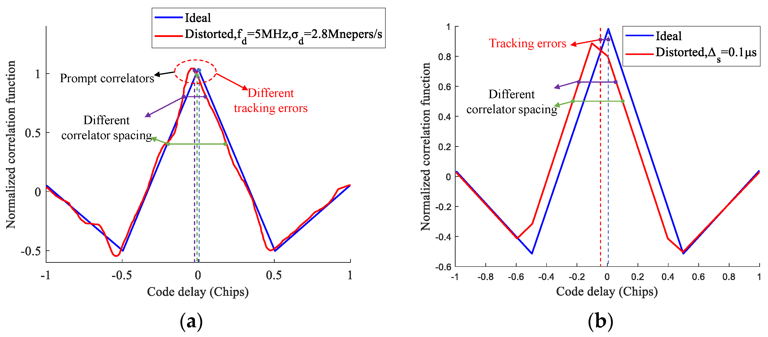
  • Threat Model A (TM-A): This type of threat is expressed as the advance or delay of the falling edge of each unit code (TC) block relative to the normal falling edge (Δ).
  • Threat Model B (TM-B): This type of threat is expressed as a 2-order step ringing response of the code block, and fd is the oscillation frequency in MHZ. σ is the damping coefficient in monap per second (MNp/s).
  • Threat Model C (TM-C): This type of threat is represented as a combination of digital distortion and analog distortion.
For signal distortion types, GPS C/A has defined some types [1], but BeiDou B1C uses its unique BOC (1,1) modulation, which needs to be redefined [2]. Since reading a lot of literature, this paper focuses on the three types of distortion of BeiDou B1C signal: analog distortion, PN code distortion, and subcarrier distortion.
The analog distortion is caused by the hardware defect of the RF module at the signal generating end, which corresponds to the previous TM-A. A common phenomenon that produces analog distortion is amplitude modulation or ringing during chip switching [10]. The reason for the digital distortion phenomenon is due to the internal fault of the baseband generator, which corresponds to the previous TM-B. For this kind of distortion, experts and scholars have proposed some methods [11,12]. Reference [3] subdivides the digital distortion types of BeiDou B1C signals into PN code distortion and subcarrier distortion. Based on this, the literature [13] proves that the distortion of the pilot_b of the B1C signal pilot component does not affect the code tracking. In the process of signal transmission, multiple types of distortion may occur at the same time. Since these distortions are generated by different loads on the satellite, this phenomenon is less likely to occur. This paper mainly studies the signal anomaly monitoring under a single distortion. Figure 1 plots the normalized correlation function of the BOC (1,1) signal under the above three distortion types.

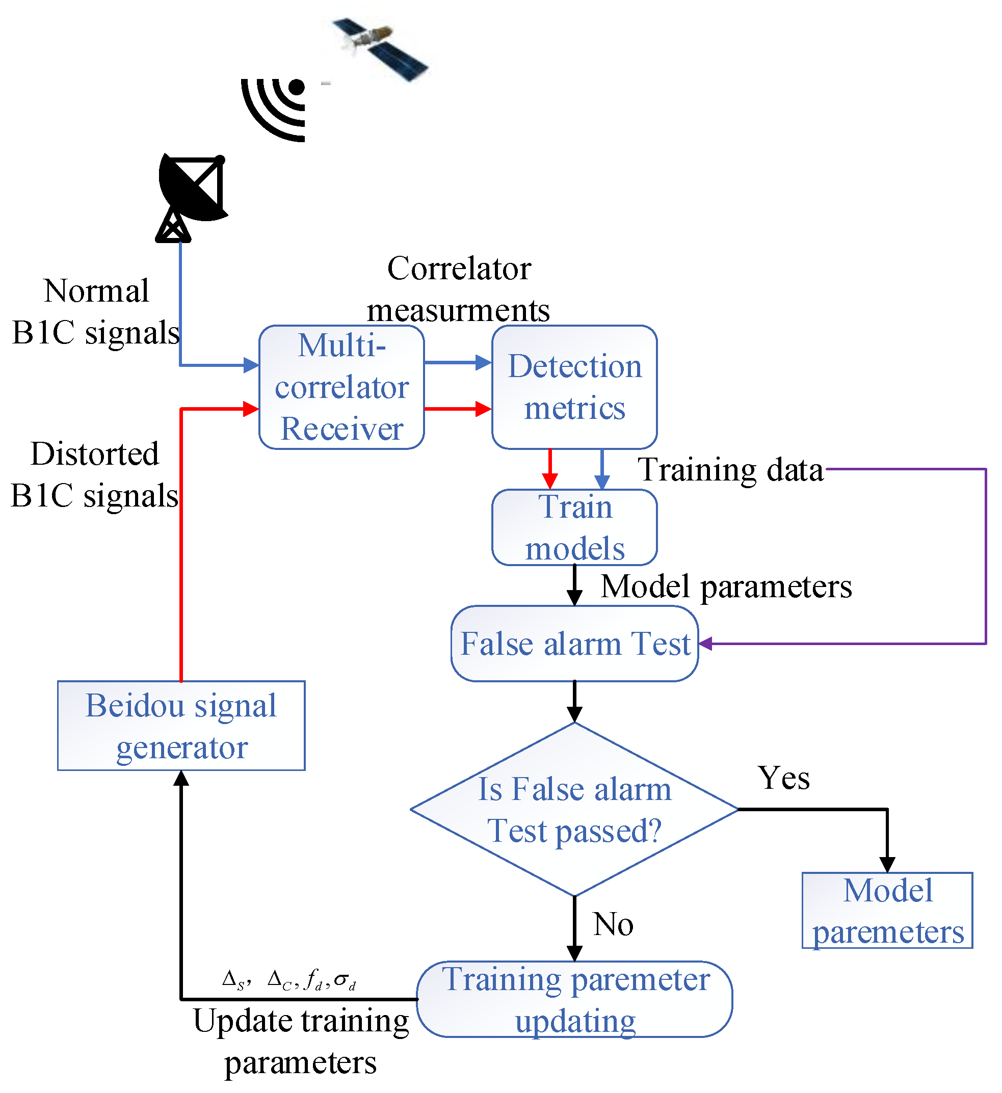
3. QDA-Based Multi-Correlator Method

In this paper, compared with traditional supervised learning methods, we propose a supervised machine learning method based on QDA. This method uses multi-correlator technology to monitor the three types of distortion of BeiDou B1C signal: analog distortion, subcarrier distortion, and PN code distortion. During quality monitoring, the discriminant method we use is quadratic discriminant analysis, which will make the discrimination more accurate. Our method is divided into two steps: offline training and online monitoring.

3.1. Offline Training

The overall flow chart of offline training is shown in Figure 2, and its input and output are the BeiDou B1C signal and the parameters of the model, respectively. The offline training process can be divided into two steps: generating a training dataset and calculating model parameters.
The training dataset is preprocessed data, which includes normal and digitally distorted BeiDou B1C signals. The feature vector X = [ X 1 , X 2 , , X d ] T of the first step, d is the dimension of the feature vector, and X i ( i = 1 ,   2 ,   , d ) is some detected feature metrics. The feature metric consists of a simple scale degree M z and a delta metric M z z . A simple ratio can be expressed by Equation (4).
M z = I z I 0
where I 0 represents the measurement value of the real-time correlator, and its main function is to normalize the correlation measurement value. I z is the measurement of the in-phase correlator at a distance z from the immediate correlator. The main function of the Delta metric is to detect the asymmetry of the correlation peak, and the Delta metric can be described by Equation (5).
M z z = I z I z I 0
When the BOC signal is distorted, not only the main peak is affected, but the secondary peak will also be affected to a certain extent. In the above two characteristic measures, when z = 0.05 - n 1 m   :   m   :   0.05 ,   0.05 :   m   :   0.05 + n 1 m , M z and M z z are used to monitor the degree of asymmetry of the correlation peak of the main peak. When z = 0.05 - n 2 m   :   m   :   0.05 ,   0.05 :   m   :   0.05 + n 2 m , M z and M z z are used to monitor the relative peak asymmetry of the secondary peak. Among them, m is a fixed code delay, that is, the distance between two adjacent correlators. Metrics n1 and n2 indicate the number of correlators on the main and sub-peaks. Therefore, when the value of z changes, the combination of these characteristic metrics can monitor the correlation peak distortion of the main peak and the secondary peak at the same time, in order to monitor the signal distortion more comprehensively and accurately.
In this paper, the dataset used for training consists of a set of input instances and desired outputs. An instance of the input can be denoted as [ x 1 , x 2 , , x d ] T , where x i ( i = 1 , 2 , , d ) represents the result of the detection metric. The output space is then expressed by Equation (6).
Ω = { ω 1 , ω 2 , ω 3 , ω 4 }
where ω 1 , ω 2 , ω 3 , ω 4 represent the input signal without fault, PN code distortion, subcarrier distortion, and analog distortion, respectively. When the training data set of the model is given, the next step is the calculation of the model parameters. Thermal noise can be regarded as a Gaussian process with zero mean, so the relevant measurement values can also be regarded as a Gaussian variable, and because the ratio of the two Gaussian processes is often a Gaussian process, the monitoring indicators are also Gaussian variables. Therefore, the input composed of the above indicators can be regarded as a variable obeying a multivariate Gaussian distribution. Therefore, our model can use a multivariate Gaussian model whose parameters are the mean vector and the covariance matrix.
We use maximum likelihood estimation to calculate the parameters of the model with the conditional probability of the input data given in Equation (7).
p ( x i j ω i ) = e x p { 1 2 ( x i j μ ω i ) T ω i 1 ( x i j μ ω i ) } ( 2 π ) d 2 | ω i | 1 2
where d represents the dimension of the input matrix, μ ω i and ω i represent the given model parameters, and x i j denotes the i-th input data corresponding to the j-th distortion. The joint likelihood function can be expressed by Equation (8).
l n L ( μ ω i , ω i ) = ( d N 2 l n ( 2 π ) N 2 l n ( ω i ) 1 2 j = 1 N ( x i j μ ω i ) T ω i 1 ( x i j μ ω i ) )
The model parameters can be obtained by ML estimation:
l n L ( μ ω i , ω i ) μ ω i = 0 μ ω i = 1 N j = 1 N x i j
l n L ( μ ω i , ω i ) μ ω i = 0 ω i = 1 N j = 1 N ( x i j μ ω i ) ( x i j μ ω i ) T
From Equations (9) and (10), our model parameters contain a total of 4 means and 4 covariance matrices.

3.2. Online Monitoring

Different from the offline training process, the online monitoring process is shown in Figure 3.
The input data is the data processed by the multi-correlator. According to the model parameters trained by offline training, the entire online monitoring module can detect whether the signal is distorted. We employed quadratic discriminant analysis to identify correlation peak distortions on the test data. Quadratic discriminant analysis models the likelihood of each class as a Gaussian distribution, and then employs the posterior distribution to estimate the class to which the test data belongs.
During online monitoring and identification, the discriminant function can be calculated from the test data and offline trained parameters and can be obtained from Equation (11).
p ( x i j ω i ) = e x p { 1 2 ( x i j μ ω i ) T ω i 1 ( x i j μ ω i ) } ( 2 π ) d 2 | ω i | 1 2
where p ( ω i ) represents the prior probability of ω i , which can be expressed as p ( ω i ) = n i / ( i = 1 4 n i ) , and n i represents the number of samples corresponding to ω i . Due to the independence between p ( x ) and ω i , p ( x ) can be treated as a constant. The discriminant function in this paper uses the maximum posterior criterion probability, so it can be described by Equation (12).
argmax i = 1 , 2 , 3 , 4 p ( ω i x ) argmax i = 1 , 2 , 3 , 4 p ( x ω i ) p ( ω i )
Taking the logarithm of the discriminant function as shown in Equation (13)
l n ( p ( x ω i ) p ( ω i ) ) = ( d 2 l n ( 2 π ) 1 2 l n | ω i | 1 2 ( x μ ω i ) T ω i 1 ( x μ ω i ) + l n ( p ( ω i ) ) )
where d 2 l n ( 2 π ) is a constant term, and p ( ω i ) is also constant for each discriminant function. Therefore, the discriminant function g ω i ( x ) can be further simplified by Equation (14).
g ω i ( x ) = 1 2 l n ( | ω i | ) 1 2 ( x μ ω i ) T ω i 1 ( x μ ω i )
The decision to monitor the signal can be obtained according to the maximum a posteriori criterion probability, shown in Equation (15).
ω ( x ) = argmax ω i g ω i ( x )
where g ω i represents the corresponding distortion type. Therefore, our model can not only monitor whether the signal is distorted, but also identify the type of distortion.

4. Experimental Results

4.1. Experimental Configuration

We use a multi-correlation receiver to process the signal and measure the correlation values, the configuration of which is shown in Figure 4. The function of the filter module is to convert the radio frequency signal into an intermediate frequency signal, and then enter the digital signal processing module designed by FPGA after sampling, quantization, and digital filtering. The signal processing module can realize signal acquisition and tracking. The processed data is transmitted to the host for parameter calculation and model training.
In this paper, the distortion type of the BeiDou B1C signal is studied. The modulation method used by the B1C signal is BOC(1,1), so the parameters of the receiver are set to match the parameters of the BOC(1,1) modulation method. The correlator pair spacing is selected as 0.5TC. Since the symbol rate of B1C data is 100bps, the coherent integration time is selected as 10ns. The specific parameters of the receiver are shown in Table 1.
The eigenvectors we use are also composed of multiple indicators, whose composition is affected by the distance m between adjacent correlators and the number of monitoring points n1 and n2. In our experiments, based on our experience with multiple measurements, six groups of different feature vectors are used, and their specific configurations are shown in Table 2.
For training a model, the most important thing is the parameters of the model. The parameters of the model are calculated from the training parameters. The training parameters in this paper include Δ C t r , Δ S t r , f d t r , and σ d t r . The principle of selection of training parameters is based on the requirement of false alarms. The selection process is shown in Figure 5.
During the test, we added some distorted signals and the B1C signal of BeiDou-3 M2 for evaluation. First, we test the performance of the proposed method for distortion detection. We then further analyze the effect of changing the eigenvectors on the model. Finally, we compare our algorithm with traditional methods. The results show that under the same conditions, our method has higher detection probability for the above three distortion types. At a signal-to-noise ratio of 35dB-Hz, our detection probability is almost twice that of conventional methods.

4.2. Classification Results of Three Distortions

In this section, we first show the loss function for the dataset. We used 20,000 standard BeiDou B1C signals and 20,000 faulty BeiDou B1C signals. We take 80% as the training set and 20% as the test set. The batch size is set to 128, the epoch size is 20, and all datasets are trained for 20 epochs. The loss functions of the training set and test set are obtained as shown in Figure 6, where loss represents the loss function of the training set, and val loss represents the loss function of the test set. It can be seen that the model gradually tends to be stable.
We present the classification results of the QDA-based method for three distortions. The method proposed in this paper uses the maximum value of all faults in the discriminant function to judge the fault type. For the observed data, the discrimination results are shown in Figure 7.
As shown in Figure 7, the blue, green, and red points correspond to the discrimination results of PN code distortion, subcarrier distortion, and analog distortion, respectively. The results show that our discriminant function can discriminate the three distortions very accurately. For the PN code distortion, the value of g ω 2 is larger than the value of other discriminant functions. Similarly, the discriminant function g ω i of the other two types of distortion is also significantly larger than the other discriminant function values. Therefore, our model can accurately distinguish these distorted signals.
Figure 8 is the confusion matrix when the feature vector is used for classification. The parameters of the model are set as follows: Δ C = 0.03   μ s , Δ S = 0.03   μ s , f d = 10   MHz , σ d = 0.8   Mnepers / s . The results show that our model achieves 100% classification accuracy for analog distortion, and more than 98.5% classification accuracy for PN code distortion and subcarrier distortion. Furthermore, for all three distortion types, both the missed detection rate and the false positive rate of our model remain below 1%. To sum up, our model has very good classification results for the three types of distortion, especially analog distortion, which achieves a classification result close to 100%.

4.3. Classification Accuracy of Different Feature Vectors

In the previous section we discussed the classification performance of the eigenvector X 5 , and in this section we will compare the classification performance of different eigenvectors. It can be seen from Table 2 that the parameters of the feature vector are related to the distance between the correlators and the size of the monitoring area. For example, eigenvectors X 1 , X 2 , X 3 , and X 4 have the same correlator interval, but the size of the region they monitor is different. The eigenvectors X 3 , X 5 , and X 6 have the same monitoring area size, but the interval between the correlators is not the same. This will inevitably cause their classification accuracy to be different. Therefore, we monitor the signals using different eigenvectors to compare their performance, and in the following results, we set the signal-to-noise ratio to 40 dB-Hz.
As shown in Figure 9a,b, when Δ S or Δ C is large, the classification accuracy of the method proposed in this paper for PN code distortion and subcarrier distortion can reach more than 96%. As shown in Figure 9c, when the damping frequency f d and damping factor σ d are small, the method proposed in this paper can achieve a classification accuracy of more than 99% for the simulated distortion. Additionally, our method is sensitive to damping frequency. When f d is small, our model can easily detect analog distortion, but when f d becomes large, our model will greatly reduce the effect of analog distortion detection. The reason for this phenomenon may be due to the increase in the missed detection rate.
From Figure 9 we can also see that there is little difference in classification accuracy using vectors X 1 , X 2 , and X 3 . When the correlator is further away from the main peak, it does not have much effect, because the further away it is from the main peak, the less useful signal features are. However, when we use the vector X 4 as the feature vector, the classification performance drops significantly. This shows that when the monitored area is too small, it is easy to miss some important information of related functions.
To reduce the dimensions of the feature vector and the complexity of the algorithm, there are two methods to reduce the monitoring area and increase the interval of the correlator. Figure 9 shows that when vectors X 3 and X 5 are used as feature vectors, their classification accuracy is not much different, while the performance of feature vector X 6 is significantly lower than these two vectors. The correlator required for feature vector X 5 is much less than that required for feature vector X 3 . Therefore, using the feature vector X 5 greatly reduces the complexity of the algorithm while maintaining high accuracy.

4.4. Comparison with Traditional Methods

Traditional multi-correlator methods employ thresholding decisions to detect signal distortions. This method can only detect a single type of distortion. When multiple types of distortion exist at the same time, only a specific type of distortion can be detected, and the type of distortion cannot be discriminated. The following figure shows the comparison of the detection performance of the method proposed in this paper and the traditional method.
From Figure 10a,b, for PN code distortion and subcarrier distortion, our method is almost twice as accurate as the conventional method at a signal-to-noise ratio of 35 dB-Hz. When the signal-to-noise ratio is lower than 45 dB-Hz, the accuracy of our method has a significant improvement over traditional methods. For analog distortion, our method shows a small improvement over traditional methods.

4.5. Real Signal Evaluation

After the machine learning model is trained, we use real signals for validation. The real data was collected by the BeiDou PNT system antenna located on the roof of the Research Institute building of the University of Electronic Science and Technology of China. To better evaluate our model, we selected three satellites, BDS-M2, BDS-M3, and BDS-M5. We collected satellite data between 3 and 4 September 2022 and calculated the results every 10 milliseconds. Each satellite can collect 360,000 pieces of data in one hour. According to the different elevation angles, it can be divided into three groups of data. The elevation angle of the first group is less than 25°, the elevation angle of the second group is between 25° and 45°, and the elevation angle of the third group is greater than 45°. The false alarm rate is shown in Table 3.
It can be seen that the larger the elevation angle, the lower the false alarm rate of the model, because the higher the elevation angle, the higher the signal-to-noise ratio. In addition, BDS-M3 and BDS-M5 have a higher false alarm rate than BDS-M2, which is because the real signal we add when training the model is the signal of BDS-M2. Different satellites use the same type of modulation, but their correlation functions are different, thus increasing the false alarm rate. The false positive rate of these real data is not higher than 10−5, which shows that our model has good robustness.

5. Conclusions

This paper proposes a method based on machine learning to monitor the signal quality of BeiDou B1C and uses the QDA method to discriminate. The results show that when Δ S 0.03   μ s , Δ C 0.03   μ s , and f d 10   MHz , the classification accuracy of the method proposed in this paper can reach 100%. Not only that, our method greatly reduces the missed detection rate. The traditional method considers that the distortion part must be less than 18.5% to be regarded as a distortion-free signal. In contrast, our method can reduce the missed detection rate to 0.98%. It is worth mentioning that the training parameters selected in this paper are Δ C t r = Δ S t r = 0.03   μ s , f d t r = 10   MHz , σ d t r = 0.8   Mnepers / s , and the selected feature vector is X 5 . This parameter is still applicable to most scenes, but when a more complex scene is used, this parameter may not be applicable, and a suitable set of parameters needs to be re-selected.
The semi-supervised machine learning method proposed in this paper realizes the monitoring of navigation signals. Our model can achieve a very good recognition rate when the fault type is single. However, when multiple fault types are mixed together, although our model has a higher recognition rate than the traditional model, the recognition rate of our model is still lower than that of a single fault type. The interference in the actual environment is very complex, so future research directions should focus on the identification problem under mixed fault types.

Author Contributions

Conceptualization, B.Y. and Q.Y.; methodology, L.L.; software, L.L.; validation, B.Y., J.Z. and J.Y.; formal analysis, L.L.; resources, B.Y.; data curation, J.Y.; writing—original draft preparation, L.L.; writing—review and editing, C.G.; visualization, Q.Y.; supervision, J.Z.; project administration, B.Y.; funding acquisition, B.Y. All authors have read and agreed to the published version of the manuscript.

Funding

This research was funded by [National Key R&D Program of China] grant number [No.2021YFF0603903] And The APC was funded by [No.2021YFF0603903].

Conflicts of Interest

The authors declare no conflict of interest.

References

  1. Mitelman, A.; Phelts, R. A real-time signal quality monitor for GPS augmentation systems. In Proceedings of the 13th International Technical Meeting of the Satellite Division of The Institute of Navigation (ION GPS 2000), Salt Lake City, UT, USA, 19–22 September 2000. [Google Scholar]
  2. Pagot, J.; Thevenon, P. Threat models design for new GNSS signals. In Proceedings of the 2016 International Technical Meeting of The Institute of Navigation, Monterey, CA, USA, 25–28 January 2016. [Google Scholar]
  3. Sun, C.; Zhao, H. A Novel Digital Threat Model and Effect Analysis on Modernized BeiDou Signals. In Proceedings of the 2016 International Technical Meeting of The Institute of Navigation, Monterey, CA, USA, 25–28 January 2016. [Google Scholar]
  4. Pagot, J.; Julien, O. Signal Quality Monitoring for New GNSS Signals. Navigation 2018, 65, 83–97. [Google Scholar] [CrossRef]
  5. He, C.; Guo, J. A newevil waveforms evaluating method for new BDS navigation signals. GPS Solut. 2018, 22, 1–13. [Google Scholar] [CrossRef]
  6. Sun, C.; Cheong, J. GNSS Spoofing Detection by Means of Signal Quality Monitoring (SQM) Metric Combinations. IEEE Access 2018, 6, 66428–66441. [Google Scholar] [CrossRef]
  7. Ali, K.; Manfredini, E. Vestigial signal defense through signal quality monitoring techniques based on joint use of two metrics. In Proceedings of the IEEE/ION Position, Location and Navigation Symposium—PLANS 2014, Monterey, CA, USA, 5–8 May 2014. [Google Scholar]
  8. Phelts, R. Multicorrelator Techniques for Robust Mitigation of Threatsto GPS Signal Quality. Ph.D. Dissertation, Stanford University, Stanford, CA, USA, 2001. [Google Scholar]
  9. International Civil Aviation Organization. Aeronautical Telecommunications. Int. Stand. Recomm. Pract. 2006, 1, 55–61. [Google Scholar]
  10. Fontanella, D.; Paonni, M. A Novel Evil Waveforms Threat Model for New Generation GNSS Signals-Theoretical Analysis and Performance. In Proceedings of the ESA Workshop on Satellite Navigation Technologies and European Workshop on GNSS Signals and Signal Processing (NAVITEC), Noordwijk, The Netherlands, 8–10 December 2010. [Google Scholar]
  11. Sun, C.; Zhao, H. A frequency domain-based detection technique for digital distortion on GNSS signals. In Proceedings of the Institute of Navication GNSSC, Oregon, Portland, 12 September 2016. [Google Scholar]
  12. Sun, C.; Zhao, H. The IFFT-based SQM method against digital distortion in GNSS signals. GPS Solut. 2018, 21, 1457–1468. [Google Scholar] [CrossRef]
  13. Wei, K.; Cui, X. A Research on Modeling and Monitoring of New BDS B1C Signal Distortions in the Context of BeiDou Satellite Based Augmentation System. In Proceedings of the Institute of Navigation International Technical Meeting 2020, San Diego, CA, USA, 21–24 January 2020. [Google Scholar]
Figure 1. Correlation function of BOC (1,1) under three distortion types. (a) Analog distortion; (b) Subcarrier distortion; (c) PN code distortion.
Electronics 11 03201 g001aElectronics 11 03201 g001b
Figure 2. Offline training flow chart.
Electronics 11 03201 g002
Figure 3. Flow chart of online monitoring based on QDA.
Electronics 11 03201 g003
Figure 4. Selection process of training parameters.
Electronics 11 03201 g004
Figure 5. Selection process of training parameters.
Electronics 11 03201 g005
Figure 6. Loss functions for training and test sets.
Electronics 11 03201 g006
Figure 7. Discrimination results of three distortions. (a) 3D visualization of eigenvectors g ω 2 , g ω 3 , g ω 4 ; (b) 2D visualization of eigenvectors g ω 2 and g ω 3 ; (c) 2D visualization of eigenvectors g ω 3 and g ω 4 ; (d) 2D visualization of eigenvectors g ω 2 and g ω 4 .
Electronics 11 03201 g007
Figure 8. Confusion matrix of eigenvector X 5 .
Electronics 11 03201 g008
Figure 9. Classification accuracy of different feature vectors. (a) Subcarrier distortions; (b) PN code distortions; (c) Analog distortions.
Electronics 11 03201 g009
Figure 10. The algorithm in this paper is compared with the traditional method. (a) PN code distortions; (b) Subcarrier distortions; (c) Analog distortions.
Electronics 11 03201 g010
Table 1. The parameters of the receiver.
ParameterValue
Tracking techniqueE-L(BOC(1,1) local replica)
Correlator spacing0.5 TC
Front-end bandwidth16 MHz
Sampling frequency40 MHz
ADC resolution4 Bits
Coherent integration time10 ms
Table 2. Parameter configuration of eigenvectors.
ParameterValue
M
(In Chip Unit, TC)
n1
(Amount)
n2
(Amount)
X 1 0.021010
X 2 0.0288
X 3 0.0266
X 4 0.0244
X 5 0.0344
X 6 0.0433
Table 3. The false alarm rate of our model for different satellite data.
Test
Data Set
Satellite
BDS-M2BDS-M3BDS-M5
Group 10.0024%0.0042%0.0031%
Group 20.0007%0.0015%0.0013%
Group 30.0003%0.0009%0.0008%
Publisher’s Note: MDPI stays neutral with regard to jurisdictional claims in published maps and institutional affiliations.

