Abstract
In 2022, as a result of the historically exceptional high temperatures that have been observed this summer in several parts of China, particularly in the province of Sichuan, residential demand for energy has increased. Up to 70% of Sichuan’s electricity comes from hydropower, thus creating a sensible and practical reservoir scheduling plan is essential to maximizing reservoir power generating efficiency. However, classical optimization, such as back propagation (BP) neural network, does not take into account the correlation of samples in time while generating reservoir scheduling rules. We proposed a prediction model based on LSTM neural network coupled with wavelet transformation (WT-LSTM) to address the problem. In order to extract the reservoir scheduling rules, this paper first gathers the scheduling operation data from the Xiluodu hydropower station and creates a dataset. Next, it uses the feature of the time-series prediction model with the realization of a complex nonlinear mapping function, time-series learning capability, and high prediction accuracy. The results demonstrate that the time-series deep learning network has high learning capability for reservoir scheduling by comparing evaluation indexes such as root mean square error (RMSE), rank-sum ratio (RSR), and Nash–Sutcliffe efficiency (NSE). The WT-LSTM network model put forward in this research offers better prediction accuracy than conventional recurrent neural networks and serves as a reference base for scheduling decisions by learning previous scheduling data to produce outflow solutions, which has some theoretical and practical benefits.
1. Introduction
This year, numerous locations across the nation experienced long-lasting high temperature records. As is known, the vast majority of Sichuan’s energy supply comes from hydropower; the installed capacity of hydroelectric power generation and hydroelectric power generation capacity are both rated first in the nation. However, the residents’ demand for electricity has recently increased due to the persistent dry, high temperatures; additionally, the operating water level of many hydropower stations in Sichuan has dropped, which has made the power supply situation worse than in previous years. The province’s power supply and demand situation has changed from a power “shortage” during the peak of July to a “double shortage”—one that lasts the entire day.
To solve the problem of power shortage, it is necessary, on one hand, to continuously develop hydropower resources, and on the other hand, to scientifically and effectively guide the production and life operation of these power stations in order to maximize the benefits of reservoirs [1]; this is the central research question in the field of reservoir scheduling. The scheduling in the actual operation of the power station can be either long-term or short-term, and its scheduling plan can also be viewed as scheduling guidelines, which must be continually reviewed and adjusted to the operating conditions.
Reservoir scheduling is an important measure to realize the comprehensive benefits of reservoirs and mitigate the adverse ecological impacts of water conservancy projects [2]. The timely formulation of reasonable and effective reservoir scheduling plans is essential to realize the comprehensive benefits of reservoirs and maintain the ecological health of the watershed [3]. Due to its unique implementation technique, implicit stochastic optimum scheduling is typically employed because there is a great deal of uncertainty in the future scheduling of reservoirs. The best long-term operation is a series of discrete data fitting; the fitting method requires a large amount of data, and the most straightforward and widely used method is to utilize the linear regression method. Although the scheduling function is increasingly complicated, it eventually needs to consider a nonlinear fitting function.There are many kinds of nonlinear scheduling functions, and the BP neural network is one of them. Due to its strong nonlinear mapping capabilities and adaptable network topology, the reservoir system’s input-output connection can be freely fitted at different times. The samples are assumed to be independent of one another when BP neural network is used to extract reservoir scheduling rules, and the correlation of samples over time is not taken into consideration. In recent years, there has been an increasing number of studies on the use of artificial intelligence (AI) technology to guide reservoir scheduling [4], and the main research directions are scheduling optimization, scheduling simulation, and scheduling optimization-simulation coupling. At present, the domestic research mainly focuses on the optimization of reservoir operation, and the simulation research of reservoir operation is rare, especially the optimization simulation of operation. The purpose of reservoir dispatching optimization simulation research is to learn reservoir dispatching rules more accurately and quickly from historical dispatching data and guide dispatching work [5]. Currently, the AI algorithms mainly include artificial neural networks and decision trees [6], which are mostly classed as shallow learning and therefore cannot effectively learn the scheduling rules of reservoirs in the face of complex influencing factors. For example, when BP neural networks are used to extract scheduling rules, the samples are presumed to be independent of one another, and the samples’ temporal correlation is ignored. There is a correlation between statistics in the real world, such as runoff or temperature variations over time. For such prediction problems with a sequential link to time, the performance of feedforward artificial neural networks is not sufficient. Recurrent neural network (RNN), a newly developed deep learning algorithm, has been widely used in the disciplines of hydrological and meteorological forecasting in recent years because it is effective at handling time-series problems [7]. Since reservoir scheduling is a complex time-series problem affected by many factors [8], exploring the use of RNN technology to extract scheduling rules from power plant operation data may provide a new technical approach for reservoir scheduling simulation research [9].
However, although some recurrent neural network models take into account the sequence information in a long time range, they are prone to the problem of gradient disappearance, and the prediction effect with long correlation is not good. Long short-term memory (LSTM) neural networks are RNNs with enhanced performance and can overcome the problem of gradient disappearance commonly existing in ordinary recurrent neural networks, and they have a good prediction effect for time-series with long-term and short-term correlations [10]. At present, the LSTM neural network has been explored and used in the field of traffic prediction. In 2018, Liang Chen et al. employed LSTM neural networks to explore the relationship between water level variations in Dongting Lake and the Three Gorges Dam upstream and conducted relevant experiments; the results demonstrated that the LSTM model is more accurate than support vector machine models [11]. Since then, many studies have shown that LSTM neural networks can predict the production of new wells in oil fields and the prediction results have been compared to those of support vector regression model and BP neural network; studies have concluded that the prediction model has a superior fitting effect and greater prediction accuracy. As a result of its potent learning capacity, LSTM neural networks have also been applied to load forecasting and runoff forecasting [12].
Although the LSTM model has shown good applicability in time-series prediction, due to the non-stationarity of reservoir operation time-series data and the difficulty in determining prediction model parameters, the popularization and application of data-driven models are limited, so further improvement is still needed to improve the prediction accuracy [13]. In previous studies, there are two main strategies to improve prediction accuracy: one is data preprocessing technology, which can reduce the non-stationary features of time-series data and extract effective information hidden in the data [12], and the second is to use the optimization algorithm to optimize the super parameters of the model. Therefore, in recent years, many scholars have made explorations in time-series preprocessing and model parameter optimization. Wavelet transform can transform the time-frequency space of the original sequence from the spectrum analysis, and has been widely used in data prediction. Dominguez et al. decomposed the Twitter traffic time-series by applying the discrete wavelet transform, fitting the appropriate ARIMA model, and then reconstructed the prediction time-series by using inverse wavelet transform [14]. The final results verify the feasibility of this method. Chai YC et al. combined the Mallat wavelet and BP neural network to build a short-term traffic flow prediction model, and selected average absolute error (MAE), mean square error (MSE), and equal coefficient (EC) as evaluation indicators to analyze the error structure. Finally, the detection information of Chengdu Chongqing Expressway verified that the model was superior to the traditional method [15]. Rishabh et al. proposed the discrete wavelet transform (DWT), auto regressive integrated moving averages (ARIMA) model, and the recurrent neural network (RNN)-based technique for forecasting computer network traffic, and sampled computer network traffic on computer network equipment connected to the Internet. The results showed that this method is easy to implement and has low computational cost [16]. Observed monthly rainfall time-series data was divided into eight subseries by Wenchuan Wang et al. using WPD, each with a different frequency and level of geographical and temporal resolution. The prediction for the decomposed monthly rainfall series was then completed using three data-based models, namely the BPNN, GMDH, and ARIMA models. The findings show that, in terms of the four assessment variables, WPD-BPNN may deliver the best performance during both training and testing periods [17]. The maximal overlapping discrete wavelet packet transform (MODWPT) was presented by John Quilty et al. as a preprocessing technique for hydrological prediction. The test results demonstrate that this approach can provide more precise (temporary) information, which may enhance the ability of various hydrological processes to be predicted at various time scales (such as rainfall and flow) [18]. After the sequence data is processed by wavelet transform, the decomposed sequence will have a more stable variance than the original sequence, so it can make the processed data obtain better results in the prediction of intelligent computing methods or statistical methods. The existing research has not applied the combination of wavelet transform (WT) and LSTM networks to the prediction of reservoir operation data.
In addition, with the rapid development of water conservancy information technology, the amount of hydropower plant scheduling operation data available on the Internet is increasing. Therefore, the use of web crawler technology to collect power plant operation data is of great significance for the joint scheduling of reservoir groups in terrace basins with different interests. Considering the above factors comprehensively, in this paper, we utilize WT-LSTM to guide the scheduling operation of hydropower plants, taking the Xiluodu hydropower plant as an example and relying on web crawler technology.
2. Materials and Methods
The Xiluodu Hydropower Station, which has enormous comprehensive benefits including electric generation, flood management, sand control, and improved downstream shipping conditions, is situated on the main stream of the Jinsha River in Leibo County, Sichuan Province, and Yongshan County, Yunnan Province. The third-ranked power plant in the world, Xiluodu Power Station has an installed capacity of 12.6 million kilowatts. The Xiluodu project is a crucial component of the Yangtze River’s flood control system and one of the primary engineering solutions to the Chuan River’s flood management issue. The amount of entering sand from the Three Gorges reservoir area can be decreased by more than 34% with reasonable reservoir scheduling as compared to the natural state. The reservoir’s ability to control runoff will directly enhance shipping conditions downstream, and the reservoir basin itself may be partially accessible.
Xiluodu hydropower station is located in the Jinsha River Gorge section bordering Leibo County of the Sichuan Province and Yongshan County of the Yunnan Province, and is the third largest hydropower station in the world and the second in China. The project adopts a concrete hyperbolic arch dam with a height of 285.5 m, 700 m length, 600 m normal storage level, 11.57 billion cubic meters total reservoir capacity, 6.46 billion cubic meters regulating reservoir capacity, 13.86 million KW installed capacity, and 770,000 KW individual capacity. The average annual power generation capacity is 57.12 billion kilowatts, with a total investment of 79.234 billion yuan; the project is mainly for power generation, and also has comprehensive benefits such as flood control, sand control, and improvement of downstream shipping conditions, etc.
This paper uses data of Xiluodu Hydropower Station collected every six hours from November 2012 to January 2021, with missing outgoing and incoming data from November 2012 to May 2013.
2.1. Wavelet Analysis Theory (Math.)
A constant size and changeable shape of the window characterize the time-frequency localized signal processing technique known as wavelet analysis. It is a byproduct of the growth of signal processing theory and is widely utilized in communication engineering, picture analysis, voice recognition, and other domains.
Let exist in the square integrable space of real numbers . We say that is a basis wavelet if its Fourier transform satisfies the following conditions:
With a denoting the scale factor and b denoting the translation factor, scaling and translating the basis wavelet yields a family of cluster functions.
The signal of the wavelet transform is defined as
Discretizing the scale factor and the translation factor, i.e., taking , the discrete wavelet of the signal becomes
In the processing of discrete time-series, denoted by , denote the sampling time interval, the discrete form of the wavelet transform is
2.2. Structure of Long and Short-Term Memory Neurons
The gradient disappearance issue in conventional recurrent neural networks is mostly resolved by LSTM kernels, which are neuronal structures with long- and short-term memory qualities [19]. The long-term correlation of sequences can be learned by the neural network built using the LSTM kernel. While LSTM kernels perform better for the memory function, LSTM kernels are equal to regular neurons in terms of their involvement in network construction. Figure 1 is a diagram of a typical LSTM kernel structure.
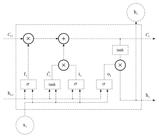
Figure 1.
Structure of LSTM kernel.
The horizontal line of the arrow at the top of the picture denotes the LSTM kernel-like Ct, which is interpreted as the LSTM kernel’s memory and conveys the information from the neuron at the previous time step to the subsequent time step. Three gates within the LSTM kernel allow for internal state modification, ensuring the kernel’s capacity for selective information filtering [20]. Sigmoid operations and multiplication operations make up the majority of gate operations. With a value of 0 rejecting all information and a value of 1 accepting all information, the data traveling through the sigmoid layer takes values between 0 and 1 to reflect the proportion of information passing through. The kernel state is multiplied by the “forgetting gate” output, which outputs a value between 0 and 1, to complete the filtering of the memory. The kernel state defines how much information needs to be deleted. The kernel output data from the previous time step and the kernel input data of the present time step are the two elements of the data involved in the “forgetting gate” calculation. The result is displayed in the below Formula (6). The weight matrices between the input data in the current time step and the output data in the previous time step and the forgetting gate are denoted by and , respectively, while the bias value employed in the calculation is denoted by .
Two factors that collectively determine which information will be maintained in the kernel state are related to the kernel state update. The “input gate” is the initial component; its value defines the percentage of candidate data that will be used for kernel state updates. It is made up of a sigmoid layer [21]. The candidate data make up the second section. The computation of , which consists of a layer that is processed through and , is in charge of producing the precise values required for kernel state updates. The function is frequently employed as the excitation function of neurons in conventional recurrent neural networks. and are displayed in the below Formula (7), where stands for the weight matrix connecting the input gate to the input data for the current time step, and stands for the weight matrix connecting the input gate to the input data for the previous time step. The weight matrices and signify the weight matrices connecting the input data and candidate data in the current time step and the output data and candidate data in the previous time step, respectively [22]. and are the offset values used to calculate and , respectively.
Kernel Status is updated according to the following Formula (8).
signifies the partial inheritance of the kernel state from the previous time step, while denotes the effect induced by the input data of the current time step. The two combined act to update the kernel state of the current time step. The computation of the kernel state is finished at this moment. The “output gate” is the final gate, which functions only on the output data from the kernel. It establishes the proportion of output data to be passed by a number between 0 and 1. The “output gate” computation is displayed in the below Formula (9). is for the weights matrix linking the output gate to the input data of the current time step and “output gate”, stands for the weights matrix connecting the output data of the previous time step and the “output gate”, stands for the bias value utilized in the calculation.
The output data of the kernel depends on the kernel state at the current time step and also needs to be filtered by the output gate as follows Formula (10).
In the above exposition and in Eq. which means the sigmoid function, and which denotes the tanh function, the specific functional form is as follows:
2.3. A Hybrid Flow Prediction Model Based on Wavelet Decomposition and Reconstruction
Forecasting and estimating daily flow and its trends is a necessary task for water resources planning and dispatching [23].In contrast to the classic network prediction models, the model of this part takes into account the trend and fluctuation prediction of hybrid flow on a broader time scale, instead of just attempting to anticipate short-term bursts of network traffic [24]. The hybrid flow sequence must display periodic variation features and the precise period length must be determined in order to develop the model. Daily hybrid flow typically exhibits cyclical volatility, and the model of this part is based on intra-day flow for modeling purposes. The various time scales of the time-series contain the variation trend and volatility characteristics of hybrid flow. Generally speaking, the volatility qualities are more pronounced on small time scales while the variation trend characteristics are more visible on large time periods [25]. Wavelet analysis demonstrates strong localization properties in both the time domain and the frequency domain, making it appropriate for the development of integrated flow prediction models. In this section, we use the wavelet transform method to analyze the flow sequences at various scales, break down the original flow sequences into a number of high-frequency and low-frequency sequences, and then use methods related to support vector machines and neural networks to learn the variation trend and volatility characteristics of the sequences to build a hybrid flow prediction model based on wavelet decomposition and reconstruction [26].
The decomposition and reconstruction prediction model put forth in this section can be broken down into three steps: the first step processes the original traffic sequence using the wavelet decomposition algorithm to produce a number of component sequences, the second step learns the characteristics of each component sequence and uses an efficient method to build the component model, and the third section’s steps make the final prediction based on the component model’s prediction outcomes [27]. Following wavelet decomposition, the traffic sequence will be split into a low-frequency approximation sequence and several high-frequency detail sequences. With the help of wavelet transform, the LSTM network can assist in identifying the differences between different signals, so as to effectively solve the problem of insufficient mining information characteristics of a single LSTM network. This study models the LSTM neural network for the approximation sequence containing the characteristics of the change trend of the original sequence and the detailed sequence containing the characteristics of the volatility of the original sequence [28].
2.4. Decomposition Reconstruction Prediction Model Design
Multiresolution analysis plays a significant role in wavelet theory. Signals are decomposed spatially using multiresolution analysis. The construction of an orthogonal wavelet basis that is closely related to the frequency of the L2(R) space is the ultimate goal of decomposition. As a result, given a signal with limited energy, the approach of multiresolution analysis can be used to separate the approximation signal and the detail signal, which can then be investigated separately depending on the situation. When creating the orthogonal wavelet basis, S. Mulat put out the idea of multiresolution analysis and also provided the renowned Mallat algorithm [14]. In wavelet analysis, the status of the Mallat method is equal to that of the rapid Fourier transform in classical Fourier transform, which has been very helpful in advancing the use and advancement of wavelet analysis. The fast Petrov–Galerkin method, the Mallat algorithm, the porous algorithm, the wavelet transform modulus based on the Hermite interpolation, and the fast wavelet transform algorithm based on the arithmetic Fourier transform are examples of common wavelet analysis algorithms. The Mallat algorithm is straightforward and user-friendly in comparison to other algorithms, and is sufficient for the purposes of this paper. The approach can combine wavelet theory with engineering applications, significantly reduce the amount of processing required for wavelet transforms, and expand the application domain.
In this section, the Mallat algorithm is adopted to decompose and reconstruct the traffic sequence. The Mallat algorithm is a signal tower multiresolution decomposition and reconstruction algorithm based on multiresolution analysis [11]. It processes the original signal by low-pass filter H and high-pass filter G. With and denoting the impulsive excitation corresponding to H and G, respectively, M denoting the number of wavelet decomposition layers, and and denoting the approximation sequence and detail sequence at scale j, the decomposition formula of Mallat algorithm is.
where denotes the impulsive response of the reconstructed low-pass filter and denotes the impulse response of the reconstructed high-pass filter, then the reconstructed equation of Mallat’s algorithm is
The decomposition and reconstruction process for handling traffic sequences with Mallat algorithm is shown in the following Figure 2.
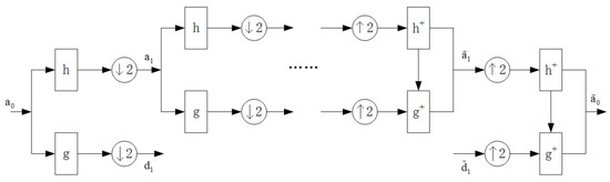
Figure 2.
Decomposition and reconstruction process of outflow sequence.
Where a0 denotes the original flow sequence, a1, d1 denote the approximation sequence and the detail sequence after one wavelet decomposition, respectively. , and denote the approximation sequence and detail sequence during wavelet reconstruction, and denotes the final sequence obtained from wavelet reconstruction.
2.5. Overall Structural Design of the Model
The decomposition and reconstruction prediction model put forward in this section is based on the theory of discrete wavelet decomposition and reconstruction, and it breaks down the flow sequence into wavelets to produce an approximation sequence with a number of detail sequences. An M-layer wavelet decomposition will eventually provide an approximation sequence with M detail sequences, since the number of sequences acquired during decomposition is inversely linked to the number of layers of wavelet decomposition [25]. Figure 3 depicts the general layout of the decomposition reconstruction model put forward in this paper.
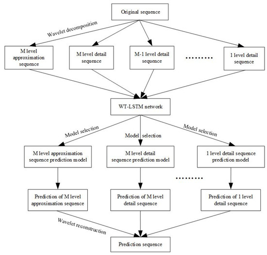
Figure 3.
Structure of the proposed prediction model.
The initial sequence in this prediction model is made up of water flow data that spans several cycles, and the prediction sequence is made up of water flow data from the following cycle. The LSTM model was used to create one of the M+1 sub-models that make up the prediction model. All of the aforementioned sub-models are trained using the component sequences produced via wavelet decomposition, and the best model is chosen as the final component prediction model after comparing the prediction outcomes.
2.6. Component Prediction Model Design
This section will specify the method of constructing the component prediction model. Let the known flow sequence be , where K denotes the number of cycles included in the full data and P denotes the number of data included in each cycle. First, the above sequence is divided into K subseries.
Decomposition of each subsequence using the wavelet decomposition algorithm yields a sequence of components of the form.
When , M denotes the number of wavelet decomposition layers, denotes the M-layer approximation sequence obtained from the jth subsequence decomposition, and denotes the M-layer detail sequence obtained from the jth subsequence decomposition. By analogy, denotes the 1-layer detail sequence obtained from the jth subsequence decomposition. Denoting Aj,m by denote the number of data points in this sequence as N. Accordingly, the number of data points within the jth subsequence Sj is approximately N*2M. Combining all the approximation sequences ( to ) into a complete sequence is denoted as . This sequence will be used to generate the training data for the LSTM neural network. The maximum data in the sequence is denoted by scale, and each data in the sequence is divided by this value to obtain the initialized sequce which is simplified as . The above data are processed into data pairs of the following form [27].
With Sub_Model(x) denoting the input-output mapping relationship of the component model, the expanded training and prediction formulas are shown in the below Formulas (17) and (18).
where denotes the corrected forecast value, which serves to prevent values with a large degree of deviation from affecting the next forecast, and the correction method is shown in the below Formula (19) where θ is an adjustable threshold parameter.
is not yet the final predicted value, the final predicted value is . Then the prediction of the final M-layer approximation sequence is , denoted as . Based on the above calculation, the prediction of the M-layer detail sequence to the 1-layer detail sequence can be obtained in the same way, and is denoted as to . The final prediction can be obtained by reconstructing the above predicted sequence using the wavelet reconstruction algorithm :
3. Experiments
3.1. Data Collection and Screening
This study uses Xiluodu hydropower station reservoir scheduling data every six hours from November 2012 to January 2021 in place of the missing outgoing and incoming data from November 2012 to May 2013. While the data’s validity is in question, operations for reservoir dispatching have been developing steadily since June 2014 and are now in accordance with the rules. The deep learning algorithm-based reservoir scheduling model was developed and trained for the time period starting on 30 June 2014, when all units were operational, and ending on 11 January 2021. The time-series of the water level change and intake and outlet flow of Xiluodu Reservoir from 2012 to 2021 is depicted in Figure 4 and Figure 5.
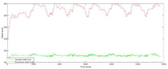
Figure 4.
Water level map of Xiluodu Reservoir from 2012 to 2021.
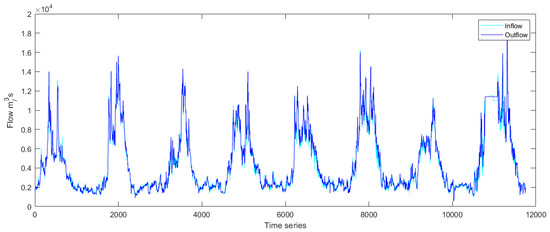
Figure 5.
Flow map of Xiluodu Reservoir from 2012 to 2021.
According to the analysis, the flow from Xiluodu Reservoir progressively increases starting in May each year, when the flood season starts and there is a lot of rainfall. The flow progressively declines after the end of October, and the non-flood season starts.
The Xiluodu hydropower station hub is made up of a barrage, facilities for electricity production, flood relief, and water diversion. The barrage is a double-bend arch dam made of concrete with a top elevation of 610 m, a maximum dam height of 278 m, and a centerline arc length of 698.09 m. The left and right banks are set up with underground plants, each with nine hydroelectric generating units with a single capacity of 700,000 kilowatts and an annual power generation capacity of 57.1 billion to 64 billion kilowatt hours. The Xiluodu Reservoir has a dead water level of 540 m and a normal storage level of 600 m. The reservoir’s overall volume is 12.67 billion cubic meters, and its regulating reservoir has a capacity of 6.46 billion cubic meters, which allows for annual partial regulation.
The hydroelectric plant at Xiluodu has numerous advantages. The primary purpose of the Xiluodu power station is to generate electricity, but it also significantly improves downstream shipping conditions, flood control, sand control, and ecology and social economics.
Efficiency of electricity generation: the Xiluodu power plant is currently not completely regulated annually. The assured output can reach 6.657 million kilowatts and the yearly power generating capacity is 64 billion kilowatt hours after the upstream terrace power station is finished. At the same time, after the power plant is finished, it can boost energy production during the dry season by 1.88 billion kilowatt-hours and enhance the guaranteed output of the power plants Three Gorges and Gezhouba by 379,200,000 kilowatts.
Benefit of sand interception: the middle reaches of the Jinsha River are one of the Yangtze River’s main sand-producing regions, and the Xiluodu dam site’s annual average sand content is 1.72 kg per cubic meter, or around 47% of the Three Gorges’ entering sand volume. Calculations and analyses show that, if the Xiluodu reservoir is run independently for 60 years, the amount of incoming sand in the Three Gorges reservoir area would be reduced by more than 34.1% compared to the natural state, and the median grain size would be refined by about 40%. This will be crucial in promoting the advantages of the Three Gorges project and minimizing the siltation of Chongqing port.
Benefits of flood control: Xiluodu reservoir has a 4.65 billion cubic meter capacity for flood control. By using the reservoir to transfer floods in conjunction with other measures, Yibin, Luzhou, Chongqing, and other cities along the Sichuan River can transition from a 20-year event to meeting the standards for urban flood control planning. When the Three Gorges reservoir is operating, the Xiluodu reservoir, which impounds the Jinsha River flood during the flood season, helps to further strengthen the Yangtze River’s middle and lower reaches’ flood control standards by directly reducing the flood volume into the Three Gorges reservoir. The study’s findings indicate that the joint operation of the Xiluodu reservoir and the Three Gorges reservoir can reduce the flood volume in the middle and lower sections of the Yangtze River by around 2.74 billion cubic meters during a 100-year flood.
Upstream navigational conditions have improved throughout the dry period: it is estimated that the dry period flow of the river section from Xinshi Town to Yibin will rise by about 500 m3/s in comparison to the natural state after the construction of Xiluodu Reservoir due to the water control and sand interception effects of the reservoir.
3.2. Input Factor Analysis
There is a water balance relationship between reservoir scheduling information such as reservoir inflow, reservoir outflow, water level above the dam, water level below the dam, and meteorological conditions such as precipitation and evaporation in the reservoir area. Month and hour information can characterize the time-series characteristics of reservoir scheduling, and the time average power plan of the power station is directly related to the reservoir’s outflow process. The model’s input factors were ultimately chosen taking into account the aforementioned variables, as given in Table 1.

Table 1.
Details of model input factors.
First, the network’s loss function was chosen. The Smooth L1 loss function, whose mathematical expression is as follows, was chosen as the network’s error function because of its higher robustness [19]. It can be calculated using the following equation: this loss function is a continuous segmentation function; it is equivalent to L2 loss function when the independent variable has values between (−1, 1) interval; it is equivalent to L1 loss function when the independent variable does not have values between the aforementioned intervals. The benefit of this segmented loss function is that it corrects both the L1 and L2 loss functions’ flaws. On one hand, it addresses the issue of the loss function’s lack of smoothness at the zero point, and on the other, it addresses the issue of gradient explosion brought on by the independent variables’ distance from the centroid [28].
Three activation functions are frequently used in deep learning: the sigmoid, tanh, and ReLU functions.
The values of (−∞, +∞) can be mapped by the sigmoid function to (0, 1). Due to the following disadvantages, the sigmoid function is not frequently utilized as a nonlinear activation function: 1. the gradient of the weights will be near to zero when x is extremely large or extremely small, which will cause the gradient update to be extremely slow, or the gradient to disappear altogether; 2. the function’s output is not mean 0, which will make it difficult to calculate the lowest layer.
More frequently than the sigmoid function, the tanh function (the hyperbolic tangent function) converts numbers with values of (−∞, +∞) to (1, 1). Within a very narrow range near 0, the tanh function can be seen to be linear. The inadequacies of the sigmoid function are compensated for by the fact that the tanh function has a mean of 0. The tanh function shares the same drawback as the sigmoid function: the gradient will be extremely small and the weights will update slowly when x is very large or very small, meaning the gradient will vanish.
The vanishing gradient issue with sigmoid and tanh functions is addressed by the ReLU function (modified linear unit), a piecewise linear function. The benefits of the ReLU function are that 1. the vanishing gradient problem does not exist when the input is positive (most of the time); 2. since the ReLU function is merely linear, it propagates information both forward and backward significantly more quickly than sigmod and tanh. A negative aspect of the ReLu function is the issue of vanishing gradient, arising when the input is negative because the gradient is zero.
Additionally, every gating unit in the LSTM network uses the ReLU function as its activation function. The weights of the gating units in the LSTM network are initialized using the Xavier technique during the initialization stage of the model training. The model’s iterative training optimization technique employs Adam’s algorithm. The network learning rate then employs the widely used exponentially decaying learning rate approach after the optimizer has been defined and a learning rate controller tied to it. To prevent any overfitting during network training, Dropout + L2 regularization + EarlyStopping is utilized, with Dropout being set to 0.5.
Thus, the regularized loss function for network training is
In the above equation, y denotes the true water level for the current month’s reservoir scheduling decision, and denotes the reservoir level at the output of the network prediction. denotes the ith weight in the network model, i denotes the number of weights, and λ is the regularization parameter, which takes values in the range [0, +∞) and is set here to 0.2. For the network output ỹ, the representation is illustrated by the following Equation (23).
In the equation above, n is the number of independent variables, and xi stands for the network input’s i-th state variable. In addition to the aforementioned network parameters, there are hyperparameters that must be decided during network training, including the number of network layers, the number of neurons in the hidden layer, the number of batches, and the size of the time window [15].
There are two typical tactics: greedy search and beam search. The greedy algorithm selects the option that is most advantageous, or the best or optimal choice under the present windowsill, at each step of the selection process, in the hopes that the outcome will also be the best or ideal. A heuristic graph search algorithm is beam search. In each step of depth expansion when the graph’s solution space is quite vast, some low-quality nodes are removed and some high-quality nodes are kept. This reduces the amount of time and space required for the search.
Greedy algorithms are especially effective when trying to solve issues with ideal substructures. The local optimal solution can determine the global optimal solution according to the optimal substructure. Correct greedy algorithms have several benefits, including minimal thought complexity, little code, great efficiency, low space complexity, etc.
In this study, we employ a greedy search strategy based on the empirical range and size of the hyperparameters and take the initiative in adjusting the hyperparameters that have the biggest impact on the network output, performing network calculations based on each preset hyperparameter, and evaluating the metrics for the prediction results until the most suitable hyperparameter size is selected, keeping the value constant after adjusting this hyperparameter, and then continuing. The task of determining parameter values is very difficult, and after numerous trials, it was discovered that the LSTM network with two hidden layers is superior to one layer (too few features cannot be learned) and three layers and above (too many network parameters are easily overfitted), since the amount of data is small. The two-layer network is also the best option [20]. The foregoing procedure of fine-tuning the parameters for the number of network layers was repeated for the other hyperparameters of the network, and the scheduling function hyperparameters were rate set for each flood season dispatching function independently.
3.3. Examining the Use of Models for Reservior Scheduling
In addition to achieving the standard accuracy requirements in terms of global errors, a successful reservoir scheduling model must be able to effectively represent specific aspects like rapid flood peaks during the flood season and very low flows during the dry season. As a result, the model’s simulation output for flood and dry periods was contrasted and examined. The models were run ten times concurrently under the assumption of optimal parameter choices, and the simulation outcomes were compared to examine the applicability scenarios for each model. The data from 1 May 2016 to 30 September 2016, and the data from 1 October 2017 to 30 April 2018 are presented here as the reservoir scheduling scenarios for the flood period and the non-flood period, respectively, due to the large number of findings.
The recurrent neural network (RNN) is a class of data that accepts sequence data as input. It is a recursive neural network in which all nodes (recurrent units) are connected in a chain, and recursion is performed in the direction of the sequence progression. The long-term reliance issue in RNN is improved by the LSTM network, and its performance is typically superior to that of the hidden Markov model and the temporal recurrent neural network (HMM). Larger deep neural networks can be built using LSTM as a complicated nonlinear unit because it is a nonlinear model. RNN is used to compare with LSTM in this paper since an enhanced LSTM network is being constructed.
When the number of hidden layers is low, the accuracy of RNN, LSTM, and WT-LSTM models are high and the distribution is more concentrated, whereas when the number of layers is high, the model accuracy decreases and the distribution is more dispersed. This is performed to investigate the impact of the number of hidden layers on the performance of the model. In terms of computation time, as the number of hidden layers rises, the model’s computation process becomes more intricate and computation time gradually increases. In order to set each model structure as having two hidden layers, the subsequent model development is unified after a thorough trade-off. The size of the training batch controls the gradient descent’s direction, which in turn impacts model performance. The test findings demonstrate that a model with a small batch value is easily diverged, and that a suitable batch value aids in the model’s quick convergence. The cause could be that when the batch value is low, the sample size of the model adjustment error gradient direction is seen as being low, and the randomness is high and challenging to converge. On the other hand, the larger the batch amount, the better the model convergence will be able to account for the global properties of the data throughout the training process, and the more accurately the direction of gradient descent will be established as a result. From the standpoint of training time, each model’s calculation time falls exponentially as the batch value rises. As a result, the training batch for all subsequent models is uniformly set to 256 under the assumption that model convergence will be achieved. The model tends to converge after there have been more than 50 iterations. After that, the model’s accuracy no longer varies dramatically with the number of iterations, and the number of iterations causes the model’s training time to steadily lengthen. In order to guarantee the model’s convergence, the number of iterations in the following construction model is uniformly set at 200.
The three deep learning time-series models can fit the actual scheduling scenario more effectively, as can be seen from Figure 5, Figure 6, Figure 7, Figure 8, Figure 9, Figure 10 and Figure 11. The WT-LSTM network is more resilient to errors and outliers than RNN and LSTM networks because it takes into consideration more information while accounting for the nonlinearity of the scheduling function. As can be shown, the reservoir operation simulated by the WT-LSTM scheduling function provides greater benefits for power generation and has strong trend prediction performance when compared to RNN and LSTM. In the real reservoir scheduling, the WT-LSTM can be utilized to determine the appropriate scheduling decision based on the particular situation of other state variables, such as the reservoir water level at the time. The output can then be assessed to see whether it is normal, increasing, or decreasing, providing a good indication of the trend. It is expected that the prediction accuracy of WT-LSTM would further increase with the accumulation of optimal scheduling techniques over several years.
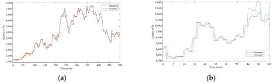
Figure 6.
Experimental results of LSTM model: (a) training set result in the flood season; (b) test set result in the flood season.
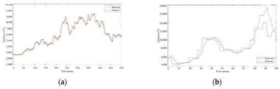
Figure 7.
Experimental results of RNN model: (a) training set result in the flood season; (b) test set result in the flood season.
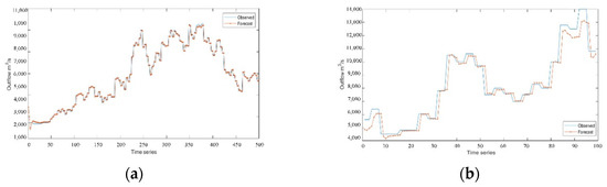
Figure 8.
Experimental results of WT-LSTM model: (a) training set result in the flood season; (b) test set result in the flood season.
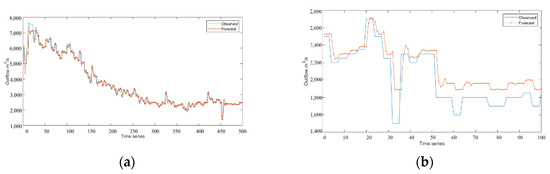
Figure 9.
Experimental results of LSTM model: (a) training set result in the non-flood season; (b) test set result in the non-flood season.
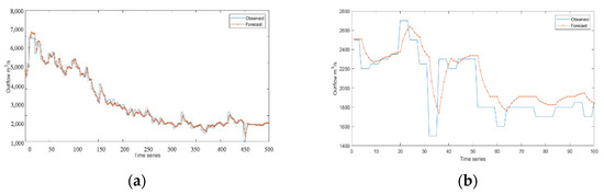
Figure 10.
Experimental results of RNN model: (a) training set result in the non-flood season; (b) test set result in the non-flood season.
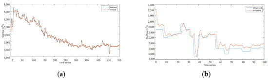
Figure 11.
Experimental results of WT-LSTM model: (a) training set result in the non-flood season; (b) test set result in the non-flood season.
3.4. Camparison of Predicted and Observed Outflow
The ranking of each model’s prediction accuracy for various hydrological periods is WTLSTM > LSTM > RNN, and the difference test of the model results for numerous simulations reveals that the difference does not reach a significant level, indicating that the three models’ prediction accuracy levels are close to one another. In addition, the three models’ prediction accuracy for non-flood seasons is higher than that of flood control during flood season. The experimental results demonstrate that all three time-series models can estimate reservoir outflows effectively and that they all have good trends for doing so.
3.5. Evaluation Metrics
Three mistakes are utilized to measure the predicting outcomes in this research in order to compare the forecasting performance of the three models mentioned above more precisely. The following formulas are used to determine the root mean square error (RMSE), rank-sum ratio (RSR), and Nash–Sutcliffe efficiency (NSE).
Standard error (or root-mean-square error, or RMSE) is the ratio of the square deviation between the observed value and its true value and the number of observations. The difference between the observed value and the true value is measured by the root mean square error. Standard errors can accurately reflect the accuracy of measurements since they are highly sensitive to very large or very small errors in a collection of measurements. The accuracy of this measuring procedure can be assessed using standard errors as a benchmark.
where denotes the true reservoir outflow, and denotes the predicted flow value.
The relative mean value of N rank for each evaluation object in the table in the multi-index comprehensive evaluation is known as the rank sum ratio (RSR) (if the weight of evaluation index is different, the index should be multiplied by the weight). RSR is a non-parametric measurement with continuous variable properties in the 0–1 range.
i indicates an object, and j indicates the serial number of each indicator.
The Nash–Sutcliffe efficiency coefficient (NSE) is generally used to verify the quality of hydrological simulation results.
The terms Qo and Qm in the formula stand for the observed value and the simulated value, respectively. Qt indicates a value at time t, while Qo stands for the sum of the observed value averages. E has a range from minus infinity to one, and when it is close to one, it means that the model is of high quality and believability. The average level of the observed values is quite near to the simulation result, meaning that the overall results are trustworthy but the process simulation error is significant when E is close to 0. If E is significantly below 0, the model is unreliable.
The above errors were calculated for the prediction results of the three models and the results are shown in Table 2. By contrasting the simulation results, the applicable situations for each model are addressed under the presumption of choosing the best settings.
Table 2.
Comparison of model performance.
The above table demonstrates that, in terms of MAE, RSR, and NSE, the prediction results of the wavelet transform-based LSTM model beat those of the LSTM model and the RNN model. This shows that the wavelet transform method and the LSTM kernel-based recurrent neural network proposed in this paper are well suited for each other, and when combined with the experimental plots, it can be demonstrated that the model can accurately and efficiently reflect the trend of the reservoir outflow and provide reliable predictions for the reservoir outflow with sudden nature. The WT-LSTM model used in the experiment is identical to other models, with the exception of the network structure, and it receives the same treatment during the training and prediction phases, as can be seen from the experimental methodology and experimental process described in the preceding section. As a result, the WT-LSTM model’s comparison environment is generally fair, and the experiment’s comparison results have high credibility and reference value. The WT-LSTM model uses more processing resources even though its prediction accuracy is greater. The LSTM model becomes more sophisticated as a result of the computation of the kernel layer and the fully connected layer, which increases the demands on resource allocation in real-world applications.
Figure 12, Figure 13, Figure 14 and Figure 15 compares the real dispatching effect with the simulated dispatching effect from the model. The figure shows that, in terms of water level requirements, the dispatching results simulated by the WT-LSTM model meet the power station’s water level requirements at various times, which is in compliance with the dispatching rules for power stations and can result in good power generation benefits.
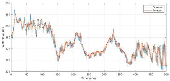
Figure 12.
Comparison of actual operating effect and simulated operating effect: WT-LSTM training result in non-flood season.
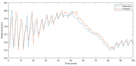
Figure 13.
Comparison of actual operating effect and simulated operating effect: WT-LSTM test result in non-flood season.
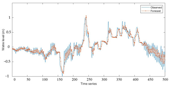
Figure 14.
Comparison of actual operating effect and simulated operating effect: WT-LSTM training result in flood season.
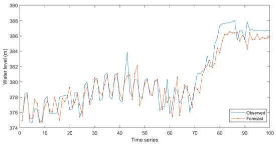
Figure 15.
Comparison of actual operating effect and simulated operating effect: WT-LSTM test result in flood season.
4. Conclusions
Scheduling models (such as linear functions and machine learning algorithms) and scheduling charts are the main tools used to schedule reservoirs, and both are simulated through extensive historical data sets. Because of its intuitive and practical benefits, the classic reservoir operation diagram is frequently used in actual operations. However, because it is rigid and does not take into account water and rain information, it has some limitations on reservoir optimization choices. Contrarily, the dispatching model extracts the reservoir dispatching rules based on the historical dispatching data of the reservoir, particularly the reservoir dispatching model based on machine learning algorithm, which can formulate a relatively flexible dispatching scheme based on the operation status of the reservoir, combined with inflow information and meteorological information, in order to significantly increase the efficiency of the reservoir. In this study, the theory of wavelet analysis is used to make the original irregular reservoir discharge series exhibit some variation features in high-dimensional space, making it possible to learn the variational laws of reservoir discharge using a time-series neural network method. A prediction model based on LSTM neural network coupled with wavelet transformation (WT-LSTM) is proposed in this paper to address the problem.
Data from the self-generating reservoir dispatch at the Xiluodu hydropower station were collected to examine the applicability of the time-series prediction model in the field of reservoir dispatch. RNN, LSTM, and WT-LSTM-based prediction models for the outflow of the Xiluodu reservoir were subsequently constructed. By contrasting evaluation indices such RRMSE, RRSR, and NNSE, the results show that the time-series deep learning network has a strong learning capability for reservoir scheduling. The experimental results show that the WT-LSTM recurrent neural network based on wavelet transform proposed in this paper has higher prediction accuracy, is able to adapt to nonlinear flow variation, offers helpful learning for unknown nonlinear flow systems, and accurately predicts low-dimensional reservoir outflow sequences.
The WT-LSTM used in this study has strong learning capabilities. When used to respond to different scenarios based on historical dispatching data from the reservoir, it can learn the dispatching rules and generate decision schemes that are remarkably similar to the actual dispatching process, which has some theoretical and practical advantages.
However, this model does still have certain flaws. The parameters used in phase space reconstruction were set by past flow data, which may not be entirely applicable to future reservoir flow. This is true even though the model can be improved over time, based on new data. More investigation and discussion are required regarding this problem’s optimization strategy. Additionally, the configuration of the number of wavelet decomposition layers is not thoroughly discussed in this study, and the degree of influence of the component sequence of each layer on the reconstructed sequence varies. The component model’s architecture can be appropriately scaled back while still maintaining acceptable levels of prediction accuracy, and the lower prediction accuracy can be sacrificed in favor of a more effective model training process. In the aforementioned areas, the model still has some space for development.
Author Contributions
Conceptualization, J.T. and R.Y.; methodology, J.T. and G.Y.; software, J.T. and G.Y.; validation, J.T., R.Y., G.Y. and Y.M.; formal analysis, J.T. and R.Y.; investigation, J.T., R.Y. and G.Y.; resources, J.T.; data curation, J.T.; writing—original draft preparation, J.T. and G.Y.; writing—review and editing, J.T. and R.Y.; visualization, G.Y.; supervision, Y.M.; project administration, Y.M. All authors have read and agreed to the published version of the manuscript.
Funding
This research was funded in part by Graduate research and innovation projects in Jiangsu Province (KYCX22 0609), and in part by the National Natural Science Foundation of China (61832005), in part by Excellent Doctoral Dissertation Cultivation Project of Hohai University (B220203006), in part by the Key Technology Project of China Huaneng Group, (HNKJ19-H12), in part by Program of the Ministry of Science and Technology of China, (2018YFC0407105).
Acknowledgments
The authors would like to acknowledge Hohai University for providing the materials used for experiments. We would like to express our gratitude to the journal editors and reviewers for the recognition of this paper, the comments and suggestions which are invaluable for the improvement of our manuscript.
Conflicts of Interest
The authors declare no conflict of interest.
References
- Simonovic, S.P.; Mariño, M.A. Reliability programing in reservoir management: 1. Single multipurpose reservoir. Water Resour. Res. 1980, 16, 844–848. [Google Scholar] [CrossRef]
- Windsor, J.S. Optimization model for the operation of flood control systems. Water Resour. Res. 1973, 9, 1219–1226. [Google Scholar] [CrossRef]
- Yu, G.; Zhang, C. Switching ARIMA model based forecasting for traffic flow. In Proceedings of the 2004 IEEE International Conference on Acoustics, Speech, and Signal Processing, Montreal, QC, Canada, 17–21 May 2004; IEEE: New York, NY, USA, 2004; Volume 2, p. 429. [Google Scholar]
- Chaves, P.; Chang, F.J. Intelligent reservoir operation system based on evolving artificial neural networks. Adv. Water Resour. 2008, 31, 926–936. [Google Scholar] [CrossRef]
- Simonović, S.P.; Mariño, M.A. The role of unconditioned and conditioned cumulative distribution functions in reservoir reliability programing. J. Hydrol. 1981, 52, 219–228. [Google Scholar] [CrossRef]
- Yang, T.; Gao, X.; Sorooshian, S.; Li, X. Simulating California reservoir operation using the classification and regression-tree algorithm combined with a shuffled cross-validation scheme. Water Resour. Res. 2016, 52, 1626–1651. [Google Scholar] [CrossRef]
- Zhang, D.; Lindholm, G.; Ratnaweera, H. Use long short-term memory to enhance Internet of Things for combined sewer overflow monitoring. J. Hydrol. 2018, 556, 409–418. [Google Scholar] [CrossRef]
- Malekmohammadi, B.; Kerachian, R.; Zahraie, B. Developing monthly operating rules for a cascade system of reservoirs: Application of Bayesian networks. Environ. Model. Softw. 2009, 24, 1420–1432. [Google Scholar] [CrossRef]
- Moeini, R.; Afshar, A.; Afshar, M. Fuzzy rule-based model for hydropower reservoirs operation. Int. J. Electr. Power Energy Syst. 2011, 33, 171–178. [Google Scholar] [CrossRef]
- Gers, F.A.; Schmidhuber, J.; Cummins, F. Learning to forget: Continual prediction with LSTM. Neural Comput. 2000, 12, 2451–2471. [Google Scholar] [CrossRef]
- Liang, C.; Li, H.; Lei, M.; Du, Q. Dongting lake water level forecast and its relationship with the three gorges dam based on a long short-term memory network. Water 2018, 10, 1389. [Google Scholar] [CrossRef]
- Chung, J.; Gulcehre, C.; Cho, K.; Bengio, Y. Empirical evaluation of gated recurrent neural networks on sequence modeling. arXiv 2014, arXiv:1412.3555. [Google Scholar]
- Moriasi, D.N.; Arnold, J.G.; Van Liew, M.W.; Bingner, R.L.; Harmel, R.D.; Veith, T.L. Model evaluation guidelines for systematic quantification of accuracy in watershed simulations. Trans. ASABE 2007, 50, 885–900. [Google Scholar] [CrossRef]
- Dominguez, G.; Guevara, M.; Mendoza, M.; Zamora, J. A wavelet-based method for time series forecasting. In Proceedings of the 2012 31st International Conference of the Chilean Computer Science Society, Valparaiso, Chile, 12–16 November 2012; IEEE: New York, NY, USA, 2012; pp. 91–94. [Google Scholar]
- Yanchong, C.; Darong, H.; Ling, Z. A short-term traffic flow prediction method based on wavelet analysis and neural network. In Proceedings of the 2016 Chinese Control and Decision Conference (CCDC), Yinchuan, China, 28–30 May 2016; IEEE: New York, NY, USA, 2016; pp. 1034–7030. [Google Scholar]
- Madan, R.; Mangipudi, P.S. Predicting computer network traffic: A time series forecasting approach using DWT, ARIMA and RNN. In Proceedings of the 2018 Eleventh International Conference on Contemporary Computing (IC3), Noida, India, 2–4 August 2018; IEEE: New York, NY, USA, 2018; pp. 1–5. [Google Scholar]
- Wang, W.; Du, Y.; Chau, K. A Comparison of BPNN, GMDH, and ARIMA for Monthly Rainfall Forecasting Based on Wavelet Packet Decomposition. Water 2021, 13, 2871. [Google Scholar] [CrossRef]
- Quilty, J.; Adamowski, J. A maximal overlap discrete wavelet packet transform integrated approach for rainfall forecasting—A case study in the Awash River Basin (Ethiopia). Environ. Model. Softw. 2021, 144, 105119. [Google Scholar] [CrossRef]
- Cardoso, A.; Vieira, F.H. Adaptive estimation of Haar wavelet transform parameters applied to fuzzy prediction of network traffic. Signal Process. 2018, 151, 155–159. [Google Scholar] [CrossRef]
- Xue, Z.; Xue, Y. Multi long-short term memory models for short term traffic flow prediction. IEICE Trans. Inf. Syst. 2018, 101, 3272–3275. [Google Scholar] [CrossRef]
- Lee, Y.J.; Min, O. Long short-term memory recurrent neural network for urban traffic prediction: A case study of Seoul. In Proceedings of the 2018 21st International Conference on Intelligent Transportation Systems (ITSC), Maui, HI, USA, 4–7 November 2018; IEEE: New York, NY, USA, 2018; pp. 1279–1284. [Google Scholar]
- Chunmei, Z.; Xiaoli, X.; Changpeng, Y. The research of method of short-term traffic flow forecast based on ga-bp neural network and chaos theory. In Proceedings of the 2nd International Conference on Information Science and Engineering, Hangzhou, China, 4–6 December 2010; IEEE: New York, NY, USA, 2010; pp. 1617–1620. [Google Scholar]
- Farajpanah, H.; Lotfirad, M.; Adib, A. Ranking of hybrid wavelet-AI models by TOPSIS method for estimation of daily flow discharge. Water Supply 2020, 20, 3156–3171. [Google Scholar] [CrossRef]
- Wang, X.; Zhang, C.; Zhang, S. Modified Elman neural network and its application to network traffic prediction. In Proceedings of the 2012 IEEE 2nd International Conference on Cloud Computing and Intelligence Systems, Hangzhou, China, 30 October 2012–1 November 2012; IEEE: New York, NY, USA, 2012; Volume 2, pp. 629–633. [Google Scholar]
- Shao, H.; Soong, B.H. Traffic flow prediction with long short-term memory networks (LSTMs). In Proceedings of the 2016 IEEE region 10 conference (TENCON), Singapore, 22–25 November 2016; IEEE: New York, NY, USA, 2016; pp. 2986–2989. [Google Scholar]
- Graves, A. Long short-term memory. In Supervised Sequence Labelling with Recurrent Neural Networks; Springer: Berlin/Heidelberg, Germany, 2012; pp. 37–45. [Google Scholar]
- Tian, Y.; Pan, L. Predicting short-term traffic flow by long short-term memory recurrent neural network. In Proceedings of the 2015 IEEE International Conference on Smart City/SocialCom/SustainCom (SmartCity), Chengdu, China, 19–21 December 2015; IEEE: New York, NY, USA, 2015; pp. 153–158. [Google Scholar]
- Fu, R.; Zhang, Z.; Li, L. Using LSTM and GRU neural network methods for traffic flow prediction. In Proceedings of the 2016 31st Youth Academic Annual Conference of Chinese Association of Automation (YAC), Wuhan, China, 11–13 November 2016; IEEE: New York, NY, USA, 2016; pp. 324–328. [Google Scholar]


Publisher’s Note: MDPI stays neutral with regard to jurisdictional claims in published maps and institutional affiliations. |
© 2022 by the authors. Licensee MDPI, Basel, Switzerland. This article is an open access article distributed under the terms and conditions of the Creative Commons Attribution (CC BY) license (https://creativecommons.org/licenses/by/4.0/).