Power Quality Disturbance Recognition Using Empirical Wavelet Transform and Feature Selection

Abstract

With the growth of nonlinear electrical equipment, power quality disturbances (PQDs) often appear in electrical systems. To solve this, a practical heuristic methodology for PQD detection and classification based on empirical wavelet transform has been proposed. By using a multiresolution analysis tool, empirical wavelet transform, the voltage waveform signal is decomposed into several sub-signals, and some potential features are extracted in the statistical method. To reduce the feature vector dimensions, the ReliefF algorithm is used for feature selection and optimized for dimensionality reduction, which reduces the complexity of system calculation while ensuring accuracy. Finally, a classifier based on support vector machines (SVM) was built, and with the ranked feature vectors’ input, the PQD can be recognized. The experimental results verify that the classification results achieved high accuracy, which confirms the properties and robustness of the proposed approach in noisy environments.

1. Introduction

Power quality disturbances (PQDs) are generated with the growth of nonlinear loads, such as solid-state switching equipment, electronically switched devices, industrial rectifiers, and inverters. Warped voltage waveforms adversely affect electronic devices, such as electrical system failures, disk crashes, and microcontroller failures [1]. Therefore, it is essential to evaluate the power quality of the electric system by recognizing detailed disturbance events. By recognizing power quality events, an efficient strategy can be carried out to stabilize power grids. The patterns and the reasons for PQDs are multiple. For example, a short trouble may result in a voltage fluctuation, which creates sag or other events [2]. The use of DC–AC inverters may result in harmonics. High-power cost equipment may lead to voltage flickers. Transient and spike events may be caused by electric discharge or sudden switching-off with overrides.

In this paper, a new algorithm is proposed for PQD detection and classification on an experimental microgrid platform. Considering the deficiencies in the reviewed literature, this proposed method is based on the EWT for decomposition, permutation entropy, and the ReliefF algorithm to obtain the relative classification features. The inspiration for the proposed approach comes from [3], in which the EWT applies three practical criteria to segment the noisy and nonstationary signal spectrum. In particular, the proposed method is based on five steps: analytical PQD signal generation, signal segmentation, feature extraction, feature selection, and pattern classification. By using a multiresolution analysis tool, an enhanced empirical wavelet transform, the voltage waveform signal is decomposed into several sub-signals. Then, some potential features are extracted from decomposed signals in the statistical method. To reduce feature vector dimensions, permutation entropy and ReliefF algorithm are used for feature selection. Finally, the optimal features are selected as the input of the SVM model to prove PQ recognition. Several experiments are performed on both simulation data and a real test platform to verify the effectiveness of the proposed method.

The main contributions of this article are as follows:

(1)

Compared with EMD, the EWT is more suitable and robust to a segmented PQD signal, especially in the selection of decomposed parameter optimization.

(2)

Based on experiment results, the permutation entropy and ReliefF algorithm are vital for feature selection, which help to filter the significant components, eliminating redundant features.

(3)

The proposed algorithm observes the characteristics of the PQD signal from a multiresolution perspective and improves the robustness and the precision of the classifier model.

2. Related Work

Different studies have been promoted for detecting power quality events. Most PQD-detecting solutions are implemented with the following processes: feature extraction, feature dimension optimization, and pattern recognition. Feature extraction is essential for PQD classification. It is noted that features can be extracted directly from the original signal or the transformed formalization. Fourier transform (FT) is a famous method, but only suitable for stationary signal processing. In other words, FT cannot resolve local information with fluctuations or transient components. Short-time Fourier transform (STFT) utilizes a sliding window on the original signal. Then, the small slice signal can be treated as many small stationary segments for FT analysis. However, time–frequency resolutions are settled along with the determined window size [4]. In [5], the authors combine wavelet transforms (WTs) to characterize PQD events. Additionally, it was certified that WT performance is better in less-noisy environments but sensitive to noise interference when detecting PQDs [6]. In a practical scene, the noises are always coupled with PQD signals, which would limit the application of a WT based algorithm. Hence, it is urgent to search for an effective multiresolution decomposition method with noisy-tolerance robustness.

To overcome the problems of the algorithms referred to above, S-transform (ST) is imported as an optimal time–frequency analysis tool by utilizing an adaptive Gaussian window. In [7,8], Mahela et al. and He et al. presented a method for PQD classification by adopting ST, respectively. In [9], the ST technique was combined with long short-term memory network structures for automatic PQD classification. Furthermore, an S-transform connected with a fuzzy system for PQD recognition was presented in [10]. Moreover, wavelet packet transform (WPT) is also popular in PQD detection due to its excellent performance [11,12]. These referred algorithms have achieved in PQD events recognition. Nevertheless, it is known that STFT, ST and WPD all utilized a fixed transform base for signal decomposition. They may be effective only in some specific scenario due to its fixed decomposition. Therefore, recently, the adaptive decomposition algorithm has been widely used in signal processing. For instance, empirical mode decomposition (EMD) shows excellent local adaptive performance in PQD research. In [13], Manjula et al. employed EMD to recognize voltage sag disturbances. The core of EMD is that it decomposes a nonstationary signal into monocomponent and symmetric signals, which are called intrinsic mode functions (IMFs). In [14], the authors investigated ensemble empirical mode decomposition performance for PQD signal processing. Although EMD has achieved many successes in PQD detection, the restriction cannot be ignored for practical application. To be specific, some IMFs cannot reveal effective details in frequency domains. Additionally, most decomposed IMFs are not analytical in mathematical theory.

Considering modal aliasing and a lack of mathematical applications, Gilles [15] developed empirical wavelet transform (EWT) to decompose a signal based on wavelet transform and spectrum dividing. The core idea of EWT is utilizing the local maximum criterion to divide the spectra into several segmentations. Then, a series of wavelet filters can be adopted to adaptively reconstruct different sub-components from the target signal. In [16,17], EWT is used to analyze voltage and current signals for PQD recognition. As concluded from the experimental results, it was noted that the EWT produces a better result than DWT and WPT in terms of the percentage of errors. Additionally, the modes revealed by the EWT benefit in terms of feature extraction.

Thereafter, the features can be extracted from the processed signals, which reveal significant information for PQDs. Common statistical features include root-mean-square values (RMS), variances, standard deviations, means, ranges, maximum values, minimum values, skewness, kurtosis, and entropies [18]. Then, the extracted features are fed into a classifier model to recognize different PQD events. Decision tree (DT), support vector machines (SVM), and artificial neural networks (ANNs) are widely used for PQD classification [19]. In [20], Naderian et al. proposed a novel algorithm to detect PQ events by combining Discrete Gabor Transform with Type-2 Fuzzy Kernel-based Support Vector Machine. Liu et al. utilized ensemble empirical mode decomposition and Ranked Wavelet SVM to classify complex PQD events [21]. In [22], authors adopted WT, hyperbolic S-transform, and DT to detect PQD events on modified Nordic 32-bus test systems. Experimental results revealed that the proposed algorithm showed better classification accuracy. In [23], an ST combined with an ANN classifier in conjunction with a Kalman filter based on maximum likelihood was developed to recognize PQD events. The ANN exhibits superior performance but struggles in small sample learning problems. The DT requires less training samples but may produce a complex model with less generalization, which would lead to a overfitting result. Compared with these classification methods, the SVM shows excellent performance for the following reasons: nonlinear classification boundary, comparatively multi-dimensional space, dependent data.

Through the literature review, numerous works have achieved outstanding results, but several limitations still exist. For instance, most of the research has discussed the importance of signal processing and feature extraction. Feature-extraction algorithms are usually based on experiential knowledge or are directly handcrafted. Unfortunately, few studies developed feature selection algorithms for PQD recognition. It is apparent that not all features are valid for classifier models. Redundant features carrying useless information may decrease PQD classification accuracy and increase the computational expense.

3. Theoretical Background

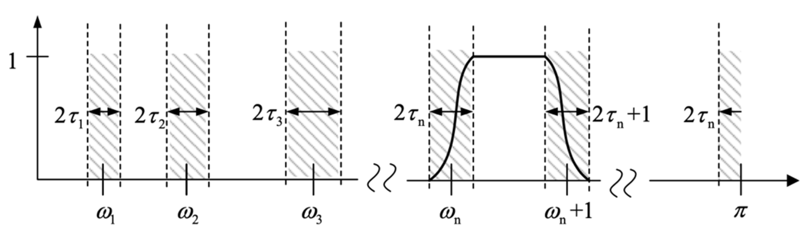
3.1. Basic Theory of Empirical Wavelet Transform

EWT’s main principle is decomposing a signal f(t) into several intrinsic mode functions (IMFs) based on wavelet transform and spectrum dividing. According to the local maximum characteristics in frequency spectrums, a series of wavelet filters are adaptively adopted to extract different IMFs. The extracted IMFs are defined as c_k. Additionally, a residual error, defined as r_n, is reserved after decomposition. Specifically, the frequency spectrum of the target signal is adaptively segmented based on local maximum values by conducting empirical wavelet filters. Then, the separation of AM–FM components in the Fourier domain is concluded. Among them, the instantaneous frequency and the instantaneous amplitude are procured from the AM–FM module by Hilbert transformation. Based on the definition, EWT has a clear wavelet theoretical framework, which avoids modal aliasing in EMD. Moreover, the decomposed IMFs are explicable for further processing.

$$f(t)={\displaystyle \sum _{k=1}^N{c}_k}+r_n$$

(1)

To adaptively separate the Fourier spectrum, the signal is divided into N-continuous components, and the local maximum values in the spectrogram are detected and arranged in descending order. Then, we can use the midpoint of two consecutive maxima as the boundaries for segments. As shown in Figure 1, the spectrum range is limited to between 0 and π, and the boundary of each adjacent segment is defined as ω_n. Meanwhile, we can define a transition zone with a width of T_n = 2τ_n. Each segment is expressed as between ω_n−1 and ω_n as Equation (2).

$$\begin{array}{l}{\Lambda }_n=\left[{\omega }_{n-1},{\omega }_n\right],\hspace{0.17em}\hspace{0.17em}\hspace{0.17em}\hspace{0.17em}n=1,2,\cdots ,N\\ {\cup }_{n=1}^N{\Lambda }_n=\left[0,\pi \right]\end{array}$$

(2)

The Meyer wavelet is selected by Gilles [15] based on the construction criterion. The empirical scale function and the empirical wavelet function are defined as Equations (3) and (4), respectively.

$${\widehat{\psi }}_n\left(\omega \right)=\{\begin{array}{c}\begin{array}{ccc}1\hfill & ,& \left|\omega \right|\hfill \end{array}\le \left(1-\gamma \right){\omega }_n\hfill \\ \cos \left[\frac{\pi }{2}\beta \left(\frac{1}{2\gamma {\omega }_n}\left(\left|\omega \right|-\left(1-\gamma \right){\omega }_n\right)\right)\right]，\hfill \\ \left(1-\gamma \right){\omega }_n\le \left|\omega \right|\le \left(1+\gamma \right){\omega }_n\\ \begin{array}{ccc}0\hfill & ,\hfill & \mathrm{others}\hfill \end{array}\hfill \end{array}$$

(3)

$${\widehat{\phi }}_n\left(\omega \right)=\{\begin{array}{r}\begin{array}{ccc}1\hfill & ,\hfill & \left|\omega \right|\hfill \end{array}\le \left(1-\gamma \right){\omega }_n\hfill \\ \cos \left[\frac{\pi }{2}\beta \left(\frac{1}{2\gamma {\omega }_n}\left(\left|\omega \right|-\left(1-\gamma \right){\omega }_n\right)\right)\right]，\\ \left(1-\gamma \right){\omega }_n\le \left|\omega \right|\le \left(1+\gamma \right){\omega }_n\\ \begin{array}{ccc}0\hfill & ,\hfill & \mathrm{others}\hfill \end{array}\hfill \end{array}$$

(4)

The parameter τ_n is chosen to guarantee the transform that provides a tight frame. The function β(x) is the auxiliary function of the Meyer wavelet, which is defined as follows:

$$\beta (x)=x^4\left(35-84x+70x^2-20x^3\right)$$

(5)

$${\tau }_n=\gamma {\omega }_n$$

(6)

$$\gamma <{\min }_n\left(\frac{{\omega }_{n+1}-{\omega }_n}{{\omega }_{n+1}+{\omega }_n}\right)$$

(7)

After deriving the empirical wavelets and the scaling function, the approximated coefficients are defined as the inner product of the signal and the scaling function:

$$W_f^{\epsilon }\left(0,t\right)=\langle f,{\varphi }_1\rangle ={\displaystyle \int f\left(\tau \right)}\overline{{\varphi }_1\left(\tau -t\right)}d\tau$$

(8)

The detail coefficients are defined as the inner product of the signal and the empirical wavelets:

$$W_f^{\epsilon }\left(n,t\right)=\langle f,{\psi }_n\rangle ={\displaystyle \int f\left(\tau \right)}\overline{{\psi }_n\left(\tau -t\right)}d\tau$$

(9)

Then, the empirical modes f_k(t) decomposed from the signal are given by:

$$\begin{array}{l}{f}_0\left(t\right)=W_f^{\epsilon }\left(0,t\right)\ast {\varphi }_1\left(t\right)\\ f_k\left(t\right)=W_f^{\epsilon }\left(n,t\right)\ast {\psi }_k\left(t\right)\end{array}$$

(10)

Then, the signal reconstruction is calculated as follows, where:

$$\begin{array}{l}f\left(t\right)=W_f^{\epsilon }\left(0,t\right)\ast {\phi }_1\left(t\right)+{\displaystyle \sum _{n=1}^N{W}_f^e\left(n,t\right)\ast {\psi }_n\left(t\right)}\\ =F^{-1}\left[{\widehat{W}}_f^e\left(0,\omega \right){\widehat{\phi }}_1+{\displaystyle \sum _{n=1}^N{\widehat{W}}_f^e\left(n,t\right)\ast {\widehat{\psi }}_n\left(t\right)}\right]\end{array}$$

(11)

3.2. Permutation Entropy

As concluded from information theory, entropy is an effective method to calculate the uncertainty degree of stochastic systems. For an observation system, when the randomness increases, the entropy value increases as well. According to entropy’s definition, it can be adopted to evaluate chaotic degrees for PQD signals. Moreover, entropy is also able to qualify for feature extraction in signal processing. Specifically, permutation entropy is an effective tool in feature statistics [24]. By calculating the sequence signal in time domains, the transient features can be extracted. In another word, the permutation entropy can assess the sequence complicacy after balancing the neighboring values. According to a mathematical model, the permutation entropy is computed by the time sequence probability density function, which is similar to Shannon entropy. For a time data series x(t) with a limited length of N, where t is increased from 1 to N, a fragment can be structured by an m-order dimension. Then, the obtained fragment is ranked in an increasing sequence that is annotated as π. After, we can set the time delay as α, and the m-order fragment X is defined as follows:

$$X_i^m=\left\{x\left(i+\alpha \left(j_1-1\right)\right),x\left(i+\alpha \left(j_2-1\right)\right),\cdots ,x\left(i+\alpha \left(j_m-1\right)\right)\right\}$$

(12)

From experimental trials, the time delay parameter α is selected as 1, and the value m is selected from three to seven. Hence, the number of m-order permutations π is the factorial of m. The relative occurrence frequency of each permutation π is presented as follows:

$$p\left(\pi \right)=\frac{H\left\{X_i^m\hspace{0.17em}has\hspace{0.17em}type\hspace{0.17em}\pi ,i|1,2,\dots ,N-m+1\right\}}{N-m+1}$$

(13)

where H represents the count number. After, the permutation entropy is estimated by the probability density function for the relative frequency:

$$PE(m)=-{\displaystyle \sum _{i=1}^{m!}p\left({\pi }_i\right)\log \left(p\left({\pi }_i\right)\right)}$$

(14)

3.3. ReliefF-Based Feature Selection Method

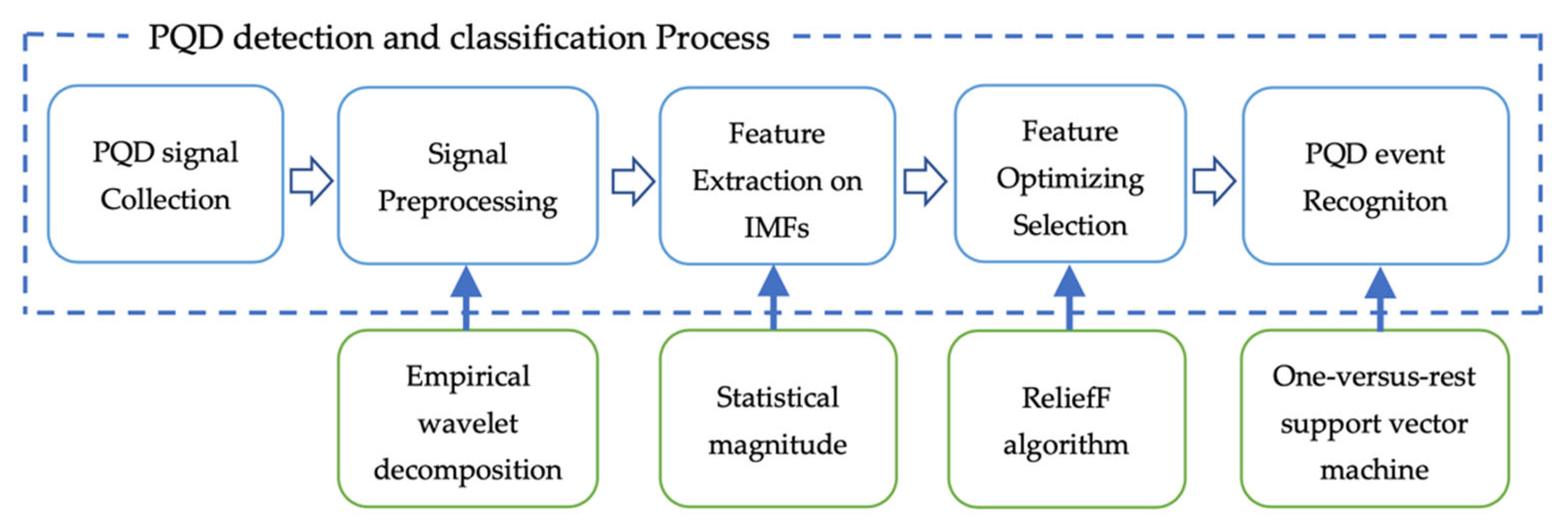
The ReliefF algorithm [25], which is a part of the Relief series, is a supervised approach for selecting features. The gap between cases from a similar classification and those from a different classification is closer for a distinguishing feature. As a result, by analyzing the relevant weight between features and classifications, the Relief algorithm can be used as a filter to select the best characteristics. The ReliefF algorithm was created to address multiclass problems because the original Relief algorithm was limited to binary classification. It is more robust and noise tolerant.

Each instance in a training dataset, D = d₁, d₂,..., d_m, has p features, which are defined as the parameter i. The i value ranges from 1 to m. The ReliefF algorithm selects an instance d_i from the dataset when utilizing binary classification. The next step is to check for two neighbors at a reasonable distance. One of the neighbors belongs to the same class as the nearest hit H, while the other belongs to a different class as the nearest miss M. For each feature t, the weight coefficient W_t is calculated as:

$$W_t=W_t-\mathit{diff}\left(t,d_i,H\right)/r+\mathit{diff}\left(t,d_i,M\right)/r$$

(15)

For numerical features, diff(t, Ri, Rj) is defined as:

$$diff(t,R_i,R_j)=\left|\frac{R_{it}-R_{jt}}{{\max }_t-{\min }_t}\right|$$

(16)

where min_t and max_t are the minimum and maximum values of feature t in dataset S, respectively. The class label for a multiclass problem is C = C₁, C₂,..., C_l. In the same class, the ReliefF algorithm looks for the k closest neighbors. Additionally, it searches for the k closest neighbors in each class.

4. Proposed Method

Figure 2 depicts the suggested methodology’s implementation process, which is broken down into five steps: PQD signal collection, signal pre-processing, feature extraction on IMFs, feature-optimizing selection, and PQD event recognition. Then, the performance of the algorithm is discussed to verify its effectiveness. Although the proposed methodology is effective in PQD recognition, it still has limitations in some application scenarios when dealing with the wrong training tags. In other words, our classifier model is obtained under supervised learning, which requires that the training samples are well-tagged. When facing wrongly tagged samples, our model may not be applicable. It is noted that this situation is universal for all supervised learning models. However, we can import a semi-supervised learning strategy, such as cooperative training, to solve this problem.

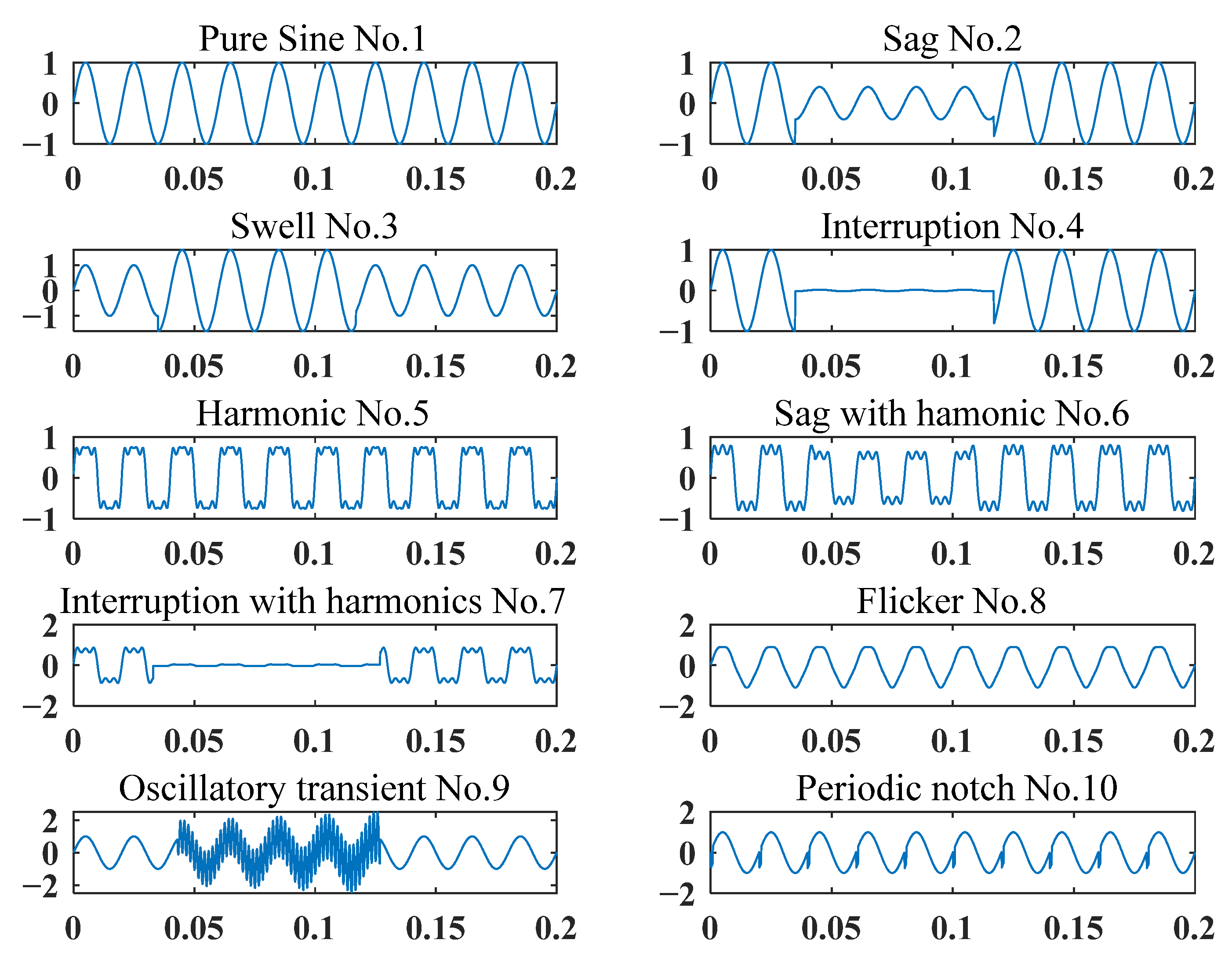
4.1. PQD Signal Simulation

Following the IEEE-1159 standard [26], a collection of signals is generated artificially in this work using mathematical models. Ten different PQD signals are selected, and the detailed models are shown in Figure 3. Specifically, the waveform is collected at 2000 data points per second at a frequency of 10 kHz. The amplitude of the fundamental sine signal, annotated as A, is normalized as 1, which randomly varies within ±10%. Moreover, to simulate real scenes, the artificial signal is coupled with Gaussian white noise. The different signal-to-noise ratios (SNRs) are set at 30 dB.

Among

Table 1. PQD mathematical model [27].

Label	PQD Type	Mathematical Model	Parameters
C1	Pure Sine	$y\left(t\right)=A\sin \left(\omega t\right)$	$\begin{array}{l}A=1\\ \omega =2\pi \ast 50\end{array}$
C2	Sag	$y\left(t\right)=A\left[1-\alpha \left(u\left(t-t_1\right)-u\left(t-t_2\right)\right)\right]\sin \left(\omega t\right)$	$\begin{array}{l}0.1\le \alpha \le 0.9\\ T\le t_2-t_1\le 9T\end{array}$
C3	Swell	$y\left(t\right)=A\left[1+\alpha \left(u\left(t-t_1\right)-u\left(t-t_2\right)\right)\right]\sin \left(\omega t\right)$	$\begin{array}{l}0.1\le \alpha \le 0.8\\ T\le t_2-t_1\le 9T\end{array}$
C4	Interrupt	$y\left(t\right)=A\left[1-\alpha \left(u\left(t-t_1\right)-u\left(t-t_2\right)\right)\right]\sin \left(\omega t\right)$	$\begin{array}{l}0.9\le \alpha \le 1;\\ T\le t_2-t_1\le 9T\end{array}$
C5	Harmonics	$y\left(t\right)=A\left[{\alpha }_1\sin \left(\omega t\right)+{\alpha }_3\sin \left(3\omega t\right)+{\alpha }_5\sin \left(5\omega t\right)+{\alpha }_7\sin \left(7\omega t\right)\right]$	$\begin{array}{l}0.05\le {\alpha }_3,{\alpha }_5,{\alpha }_7\le 0.15\\ {\displaystyle \sum {\alpha }_i^2}=1\end{array}$
C6	Sag with harmonics	$y\left(t\right)=A\left[1-\alpha \left(u\left(t-t_1\right)-u\left(t-t_2\right)\right)\right]\left[{\alpha }_1\sin \left(\omega t\right)+{\alpha }_3\sin \left(3\omega t\right)+{\alpha }_5\sin \left(5\omega t\right)\right]$	$\begin{array}{l}0.1\le \alpha \le 0.9;\\ T\le t_2-t_1\le 9T\\ 0.05\le {\alpha }_3,{\alpha }_5,{\alpha }_7\le 0.15;\\ {\displaystyle \sum {\alpha }_i^2}=1\end{array}$
C7	Interrupt with harmonics	$y\left(t\right)=A\left[1-\alpha \left(u\left(t-t_1\right)-u\left(t-t_2\right)\right)\right]\left[{\alpha }_1\sin \left(\omega t\right)+{\alpha }_3\sin \left(3\omega t\right)+{\alpha }_5\sin \left(5\omega t\right)\right]$	$\begin{array}{l}0.9\le \alpha \le 1\\ 0.05\le {\alpha }_3,{\alpha }_5,{\alpha }_7\le 0.15\\ {\displaystyle \sum {\alpha }_i^2}=1\end{array}$
C8	Flicker	$y\left(t\right)=A\left[1+{\alpha }_f\sin \left(\beta \omega t\right)\right]\sin \left(\omega t\right)$	$\begin{array}{l}0.1\le {\alpha }_f\le 0.2\\ 5\le \beta \le 20 \mathrm{Hz}\end{array}$
C9	Oscillatory transient	$y\left(t\right)=A\left[\sin \left(\omega t\right)+{\alpha }^{-c\left(t-t_1\right)/\tau }\sin \left({\omega }_n\left(t-t_1\right)t\right)\left(u\left(t_1\right)-u\left(t_2\right)\right)\right]$	$\begin{array}{l}0.1\le \alpha \le 0.8\\ 0.5T\le t_2-t_1\le 3T\\ 8 \mathrm{ms}\le \tau \le 40 \mathrm{ms}\\ 300\le f_n\le 900 Hz\end{array}$
C10	Periodic notch	$\begin{array}{l}y\left(t\right)=\sin \left(\omega t\right)-\mathrm{sign}\left(\sin \left(\omega t\right)\right)\\ \times \left\{{\displaystyle \sum _{n=0}^{9}K\times \left[u\left(t-\left(t_1-0.02n\right)\right)-u\left(t-\left(t_2-0.02n\right)\right)\right]}\right\}\end{array}$	$\begin{array}{l}0\le t_1,t_2\le 0.5T\\ 0.01T\le t_2-t_1\le 0.05T\\ 0.1\le K\le 0.4\end{array}$

, there are many parameters for PQD mathematical models [27]. The explanations are listed as follows. Symbol ω represents the fundamental angular frequency in the power grid. Symbol α is used to adjust the waveform’s amplitude. For instance, in the sag disturbance event, we set α ranging from 0.1 to 0.9. Then, the voltage amplitude would drop from 10% to 90%. Symbols t₁ and t₂ represent the start and end times for the occurring disturbances. Symbol T represents a cycle time for power grids, which is 20 milliseconds under 50 Hz. Symbol f_n represents the oscillatory frequency for the oscillatory transient event. Symbols α_f and β are used to tune the flickering shape. Symbol K is used to tune the amplitude for the notch events.

4.2. EWT Signal Segmentation

As can be observed from the mathematical models, the PQD signal is coupled with distinct components. Hence, it is essential to decompose the signal for feature extraction. In this work, the EWT is imported for signal processing. As mentioned in Section 2, the EWT can separate the objective signal into AM–FM components, which guarantees that the PQD changes can be traced more accurately. Moreover, the EWT can reserve useful components effectively and remove noisy components. The EWT parameters are optimized for PQD signals by experimental trials, which will be discussed in the following sections. In this work, the decomposition number selected is six, which means the target signal is decomposed into six segmentations in spectral domains.

4.3. Feature Extraction and Selection

After EWT decomposition, nine statistical features are extracted from the sub-components. The detailed features are listed in

Table 2. Statistical feature models.

No.	Statistical Feature	Expression
1	RMS	$\sqrt{\frac{1}{K}{\displaystyle \sum _{k=1}^K{\left[x(k)\right]}^2}}$
2	Average	${\displaystyle \sum _{k=1}^K\left[x(k)\right]}/K$
3	Standard Deviation	$\sqrt{{\displaystyle \sum _{k=1}^K{\left[x(k)-\overline{x}\right]}^2}/\left(K-1\right)}$
4	Variance	${\displaystyle \sum _{k=1}^K{\left[x(k)-\overline{x}\right]}^2}/K$
5	Range	$\max \{x(k)\}-\min \{x(k)\}$
6	Kurtosis	${\displaystyle {\sum }_{k=1}^K{\left[\left(x(k)-\overline{x}\right)/\sigma \right]}^4/K}$
7	Skewness	${\displaystyle {\sum }_{k=1}^K{\left[\left(x(k)-\overline{x}\right)/\sigma \right]}^3/K}$
8	Average Deviation	${\displaystyle {\sum }_{k=1}^K\left|x(k)-\overline{x}\right|/K}$
9	Permutation Entropy	$-{\displaystyle \sum _{i=1}^{m!}p\left({\pi }_i\right)\log \left(p\left({\pi }_i\right)\right)}$

, which is inspired by [28].

To be specific, since the PQD signal is decomposed into six IMFs, the referred nine statistical features are imported for each IMF. In other words, fifty-four features are obtained to construct feature vectors. As referred to in Equation (17), the constructed feature vectors are defined as F(i) = [F₁, F₂, …, F₉], where i is the i-th order of the data sample. F₁, F₂, …, F₉ are the RMS feature vectors, standard deviation annotated as σ, variance annotated as var, range, skewness annotated as SK, kurtosis annotated as KT, mean annotated as μ, average deviation annotated as $\overline{\sigma }$, and permutation entropy annotated as PE, respectively.

$$\begin{array}{l}{F}_1=\left[RM{S}_1\hspace{0.17em}RM{S}_2\hspace{0.17em}RM{S}_3\hspace{0.17em}RM{S}_4\hspace{0.17em}RM{S}_5 RM{S}_6\right]\\ F_2=\left[{\mu }_1\hspace{0.17em}{\mu }_2\hspace{0.17em}{\mu }_3\hspace{0.17em}{\mu }_4\hspace{0.17em}{\mu }_5 {\mu }_6\right]\\ F_3=\left[{\sigma }_1\hspace{0.17em}{\sigma }_2\hspace{0.17em}{\sigma }_3\hspace{0.17em}{\sigma }_4\hspace{0.17em}{\sigma }_5 {\sigma }_6\right] \\ F_4=\left[{\mathrm{var}}_1\hspace{0.17em}{\mathrm{var}}_2\hspace{0.17em}{\mathrm{var}}_3\hspace{0.17em}{\mathrm{var}}_4\hspace{0.17em}{\mathrm{var}}_5 {\mathrm{var}}_6\right]\\ F_5=\left[rang{e}_1\hspace{0.17em}rang{e}_2\hspace{0.17em}rang{e}_3\hspace{0.17em}rang{e}_4\hspace{0.17em}rang{e}_5 rang{e}_6\right]\\ F_6=\left[K{T}_1\hspace{0.17em}K{T}_2\hspace{0.17em}K{T}_3\hspace{0.17em}K{T}_4\hspace{0.17em}K{T}_5 K{T}_6\right]\\ F_7=\left[S{K}_1\hspace{0.17em}S{K}_2\hspace{0.17em}S{K}_3\hspace{0.17em}S{K}_4\hspace{0.17em}S{K}_5 S{K}_6\right]\\ F_8=\left[{\overline{\sigma }}_1\hspace{0.17em}{\overline{\sigma }}_2\hspace{0.17em}{\overline{\sigma }}_3\hspace{0.17em}{\overline{\sigma }}_4\hspace{0.17em}{\overline{\sigma }}_5 {\overline{\sigma }}_6\right]\\ F_9=\left[P{E}_1\hspace{0.17em}P{E}_2\hspace{0.17em}P{E}_3\hspace{0.17em}P{E}_4\hspace{0.17em}P{E}_5 P{E}_6\right] \\ F\left(i\right)=\left[F_1\hspace{0.17em}{F}_2\hspace{0.17em}{F}_3\hspace{0.17em}{F}_4\hspace{0.17em}{F}_5\hspace{0.17em}{F}_6\hspace{0.17em}{F}_7\hspace{0.17em}{F}_8\hspace{0.17em}{F}_9\hspace{0.17em}\right]\end{array}$$

(17)

One more point should be noticed in that these statistical features are calculated in different units. Therefore, the extracted features should be normalized, ranging from 0 and 1, for classifier models. As shown in Equation (18), the min–max normalization method is used in this work. Z_i is defined as the normalized data, F_i is the corresponding feature of the i-th training sample, F_max is the maximum value of the features, and F_min is the minimum value.

$$Z_{\mathrm{i}}=\frac{F_i-F_{\min }}{F_{\max }-F_{\min }}$$

(18)

Once the features are extracted, the ReliefF algorithm is adopted to select the optimal features from the original vectors. On the other hand, the feature selection algorithm can also be regarded as a dimensionality reduction. By importing the ReliefF algorithm, the vector dimensions are shortened, which benefits computational expenses.

4.4. Multiclass Pattern Recognition

In this study, the multiclass SVM is imported to recognize PQD events. Considering that the basic SVM is only able to achieve binary classification, it is essential to expand a multiclass strategy for PQD recognition. Specifically, the “one-versus-rest” (OVR) technique is widely used for multiclass categorization [27]. When facing an N-class problem, N numbers of hyperplanes are essential for the SVM classifier model. When dealing with the k-th pattern recognition, the multiclass SVM model regards the samples in the k-th class as the positive samples for training. Obviously, the rest of the samples are negative. Then, the nearest distance searching strategy is utilized to judge where the new sample belongs.

Moreover, the SVM parameters are vital for the recognition results. For this research, the radial basis function (RBF) is selected as the SVM kernel function. The RBF kernel has smooth characteristics, which are applicable for training data without prior knowledge. For the RBF, the penalty parameter, annotated as C, is used to tune the tolerance for classification error. When the penalty value is set high, it means the SVM model has a small error tolerance to the training results. In this circumstance, it may make the classifier overfitted, which means the generalization ability will be poor. Oppositely, when the penalty value is small, it means the SVM model allows a relatively large error in the classification results. In this circumstance, the SVM model may exhibit bad precision. Based on the definition, the grid search strategy is performed to optimize the penalty parameter C. After experimental trials, the penalty parameter C is selected as 25.6.

5. Experimental Results and Discussion

5.1. Experimental Setup

A microgrid platform is developed in a laboratory environment to test the suggested method as shown in Figure 4. The microgrid platform adopts a double-layer structure approach with a flexible topology, which is composed of loads, distributed power sources, and energy storage devices. Specifically, typical loads in the microgrid platform include electric motors, transmission mechanisms, induction motors, electric vehicle charging loads, and a 100 kW programmable PLC load. Additionally, distributed power sources include photovoltaic cells, photovoltaic simulators, diesel generator simulators, and wind generators, and energy storage devices consisting of lead batteries. The microgrid platform is able to work at 400 V at 50 Hz. The microgrid topology used in the simulation verification adopts the standard low-voltage microgrid system proposed by the European Union Microgrid Project (ENK5-CT-2002-00610). A variety of lines and load types can be configured in the system, with two sub-micro grid layers coupled with bidirectional converters, allowing the bidirectional flow of power transmission. More specifically, the microgrid platform can use the line impedance simulator to recreate different line faults under the logic program control.

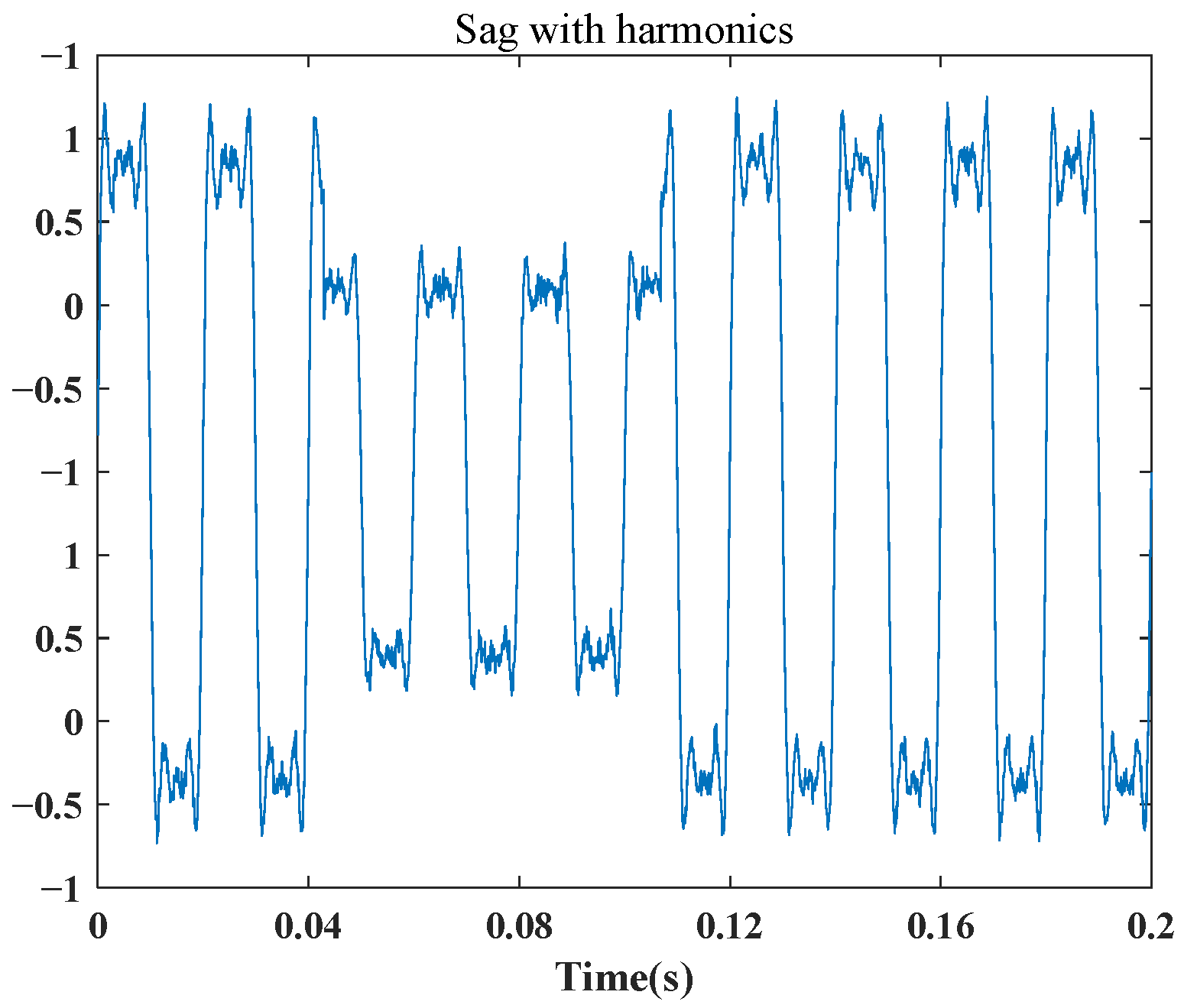
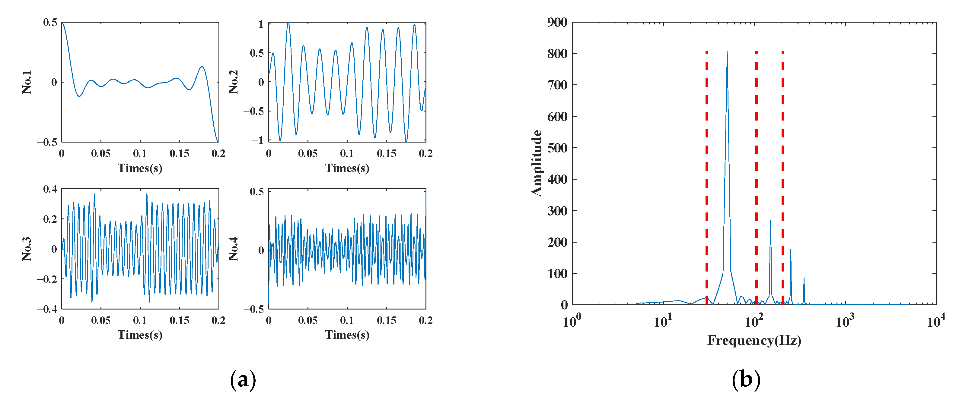
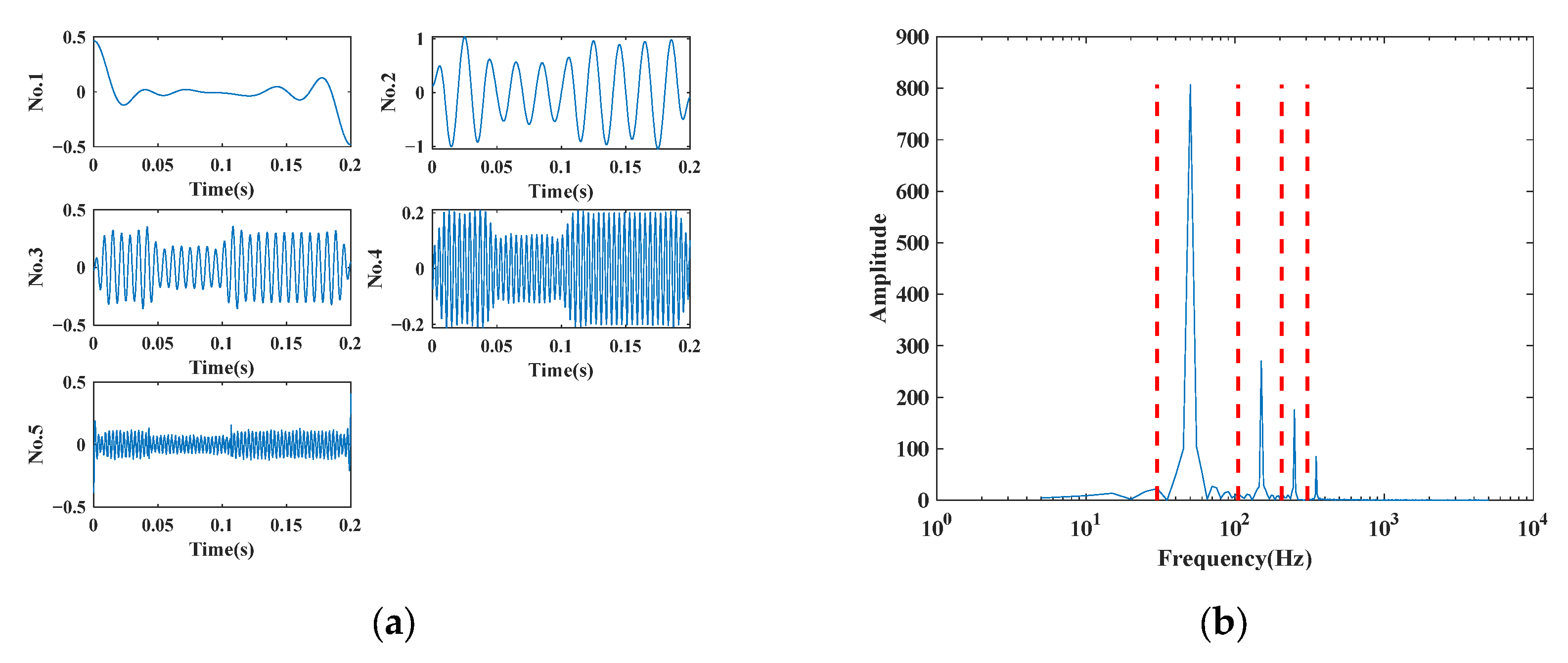
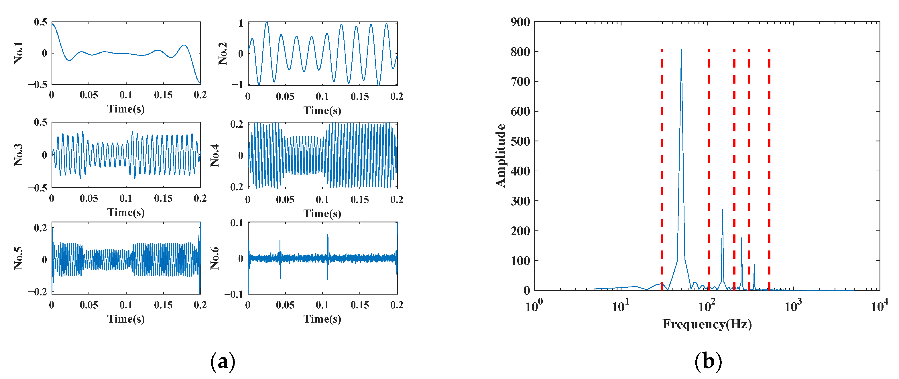
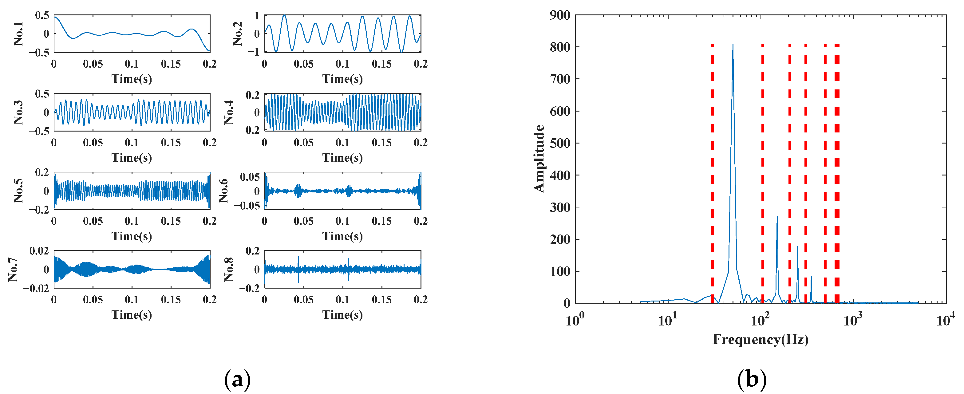
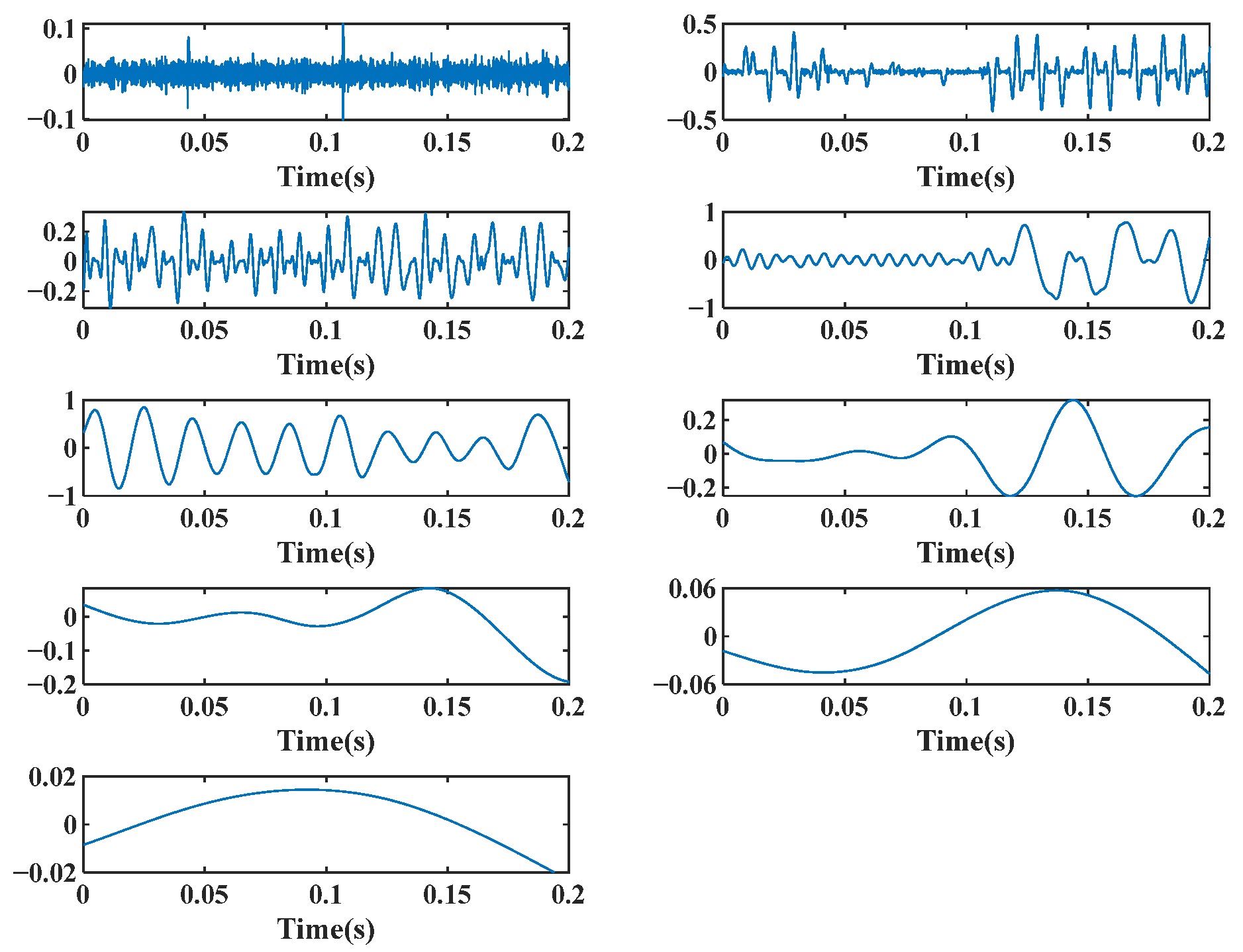
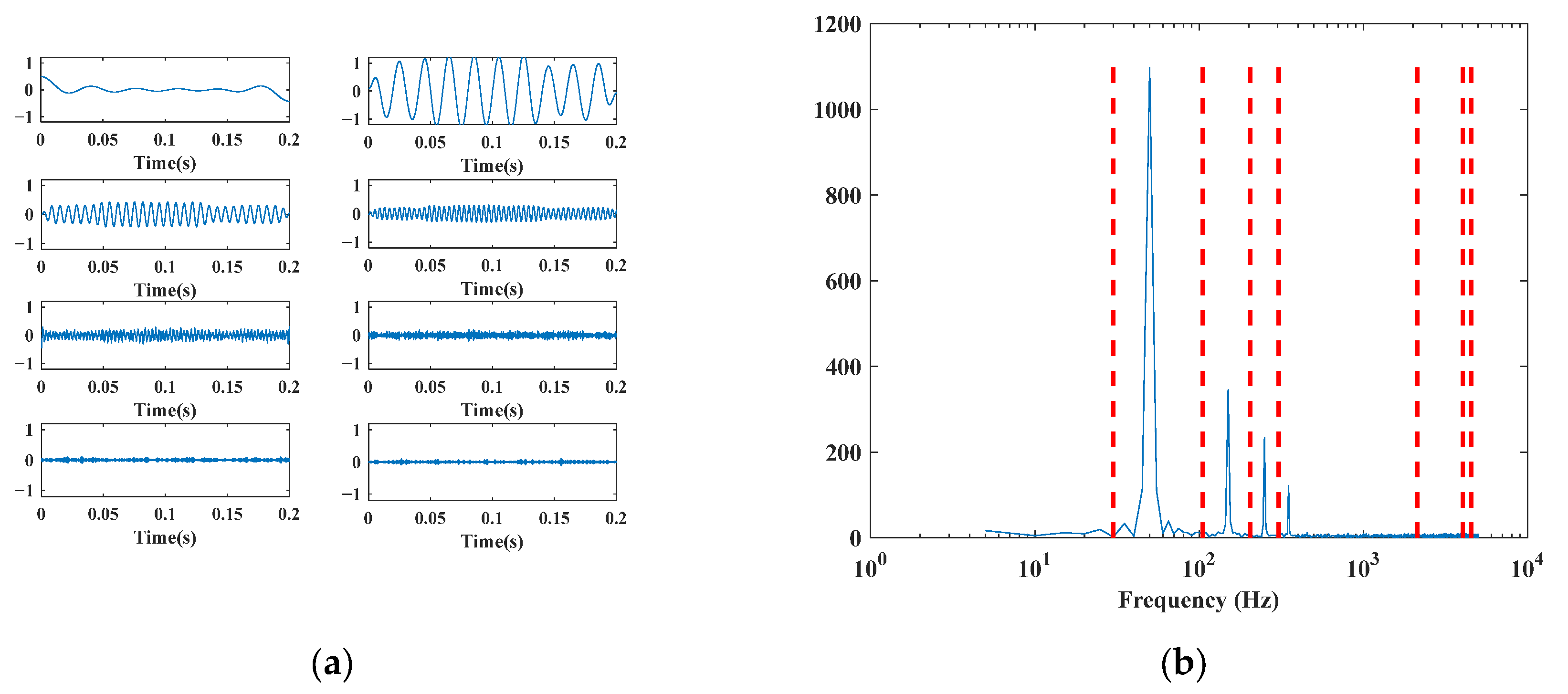
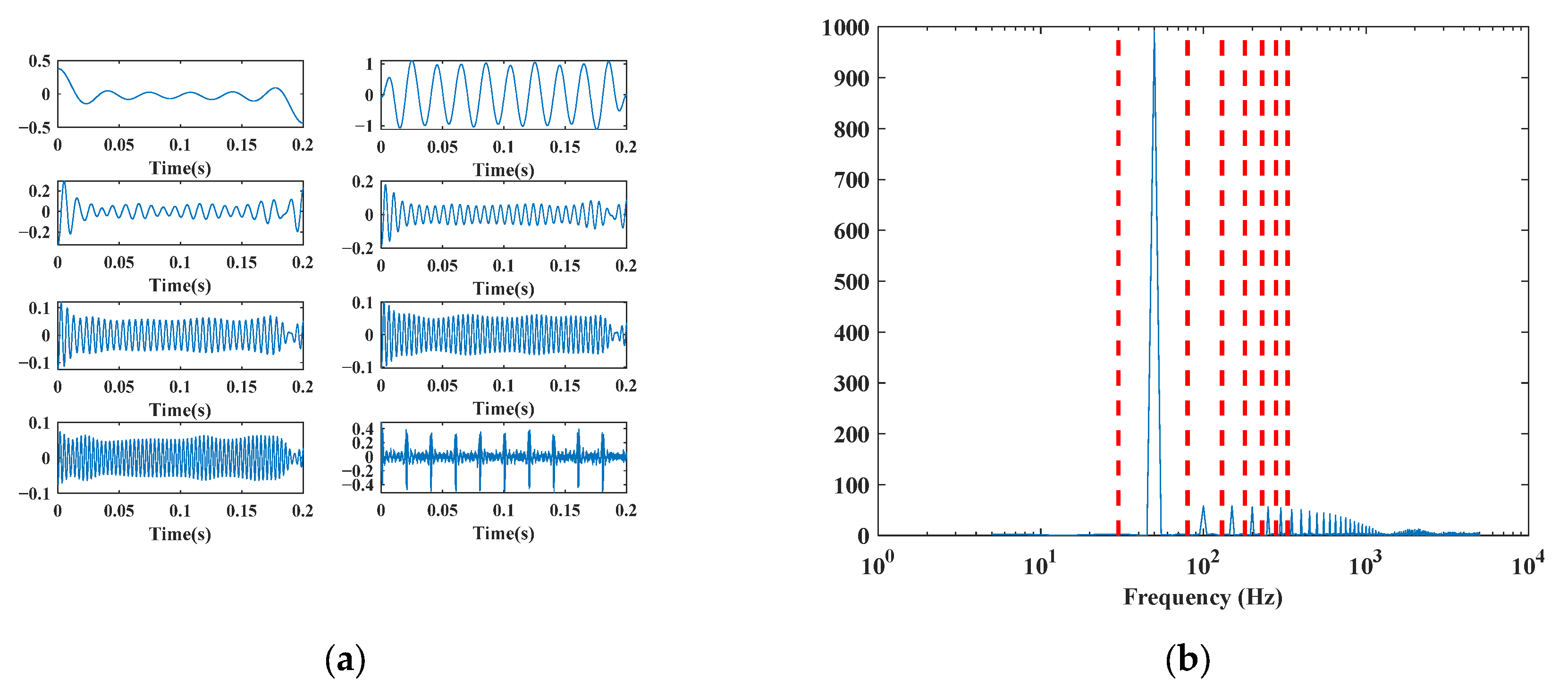
5.2. EWT Decomposition

A simulated signal representing the sag with harmonics is shown to verify the efficiency for EWT. The PQD signal waveform is presented in Figure 5. Observed from the time-series signal, the voltage sag occurs from 40 milliseconds and 110 milliseconds. Meanwhile, the signal is coupled with third, fifth, and seventh harmonics.

Figure 6, Figure 7, Figure 8 and Figure 9 show the decomposition results by EWT in time domains, where the band number N is selected as 4, 5, 6, and 8. The spectrum with segmentation lines is also shown. When N = 4 in Figure 6a, the No. 1, No. 2, and No. 3 sub-components are separated effectively in each IMF. However, the No. 4 subcomponent reveals that two different harmonics are mixed together. It is also more obvious in Figure 6b that the No. 4 spectral segmentation contains the fifth and seventh harmonics. Based on this result, it was found that the decomposition results are less decomposed. This means that the decomposition number N should increase. When N = 5 in Figure 7, although the No. 5 component still contains Gaussian noise, the decomposition results show that all the main components are separated effectively. Furthermore, there is less noise influence with the No. 2, No. 3, No. 4, and No. 5 components. Figure 8a shows that components are separated cleanly when N = 6. It is further confirmed in Figure 8b that the fundamental, third, fifth, and seventh harmonics are reserved in No. 2, No. 3, No. 4, and No. 5 spectral segmentations. Figure 8 proves that the segmentation bands are well fitted. The significant information is extracted by the EWT.

Furthermore, in Figure 9a, when N = 8, the PQD signal is over-decomposed. The key harmonics are reserved in No. 2, No. 3, No. 4, and No. 5 spectral segmentations. Interestingly, No. 6, No. 7, and No. 8 components reveal some valid information. For instance, the No. 8 component exhibits two pulses in 40 milliseconds and 110 milliseconds, which corresponds to the disturbance times. Then, we can import the entropy calculation to evaluate the chaos degree for each IMF. The permutation entropy of each IMF is 0.1246, 0.1434, 0.1980, 0.2468, 0.2874, 0.3876, 0.3868, and 0.9723, respectively. Due to the entropy analysis, the No. 8 component is chaotic and should be removed for further processing.

Moreover, as mentioned in [29], EMD is adopted to present the effectiveness of the EWT. Figure 10 presents the decomposition result by EMD. As can be observed from Figure 10, the decomposition level is nine in self-adaption. Unfortunately, most decomposed components are chaotic, and it is difficult to extract useful features. From the comparison, it was found that EMD has some limitations in PQD recognition. Specifically, the number of intrinsic mode functions (IMFs) changes according to the waveform of PQ events, which proves that the EMD does not behave well in dealing with noisy and nonstationary signals. Besides this, the decomposed IMF is not analytical compared with the IMF from EWT. According to the above analysis, the EWT is adaptable and robust for the PQD signal process, which exhibits excellent performance in mode mixing and decomposed-number-selection problems.

Additionally, two other PQD events, swell with harmonics and periodic notch, are imported to verify the effectiveness of EWT in further investigations. The results are exhibited in Figure 11 and Figure 12. In these two events, the decomposition number N is selected as eight. This is to guarantee that the PQD signal can be decomposed sufficiently. As can be observed from Figure 11 for swell with harmonics, it was found that the disturbance components are separated adaptively by EWT. The results are similar to the sag with harmonics. The difference is only in the No. 2 component. In Figure 9a, the fundamental wave at 50 Hz is reserved, while the amplitude is dropped during 40 milliseconds to 110 milliseconds. Inversely, in Figure 11a, the fundamental wave also remained, but the amplitude rose during the same time. In Figure 12, the periodic notch event is also decomposed by EWT. As can be seen from Figure 12a, it is found that the periodic notch signal consists of numerous periodic impulse components in the time domain, which is obviously detected in the frequency domain. After EWT decomposition, the key information of these PQD signals can be extracted in further processes.

As in [15], “if for a given class of signals it should be possible to guess the best number of modes, this is not the case in general where no a priori information are available”. In such cases, it is essential to estimate the appropriate number of modes. In the referred article, the author suggested offering a deeper analysis but using a simple method to estimate the number of mode N. To be specific, Gills suggested that “the most important maxima in the magnitude of the Fourier transform of the input signal (corresponding to the center of each desired Fourier segments) are significantly larger than the other existing maxima”. In this framework, the above idea is equivalent to keep all maxima that are greater than the amount of the difference between the bigger maximum and the smaller maximum. We can formulate this as “keeping all maxima larger than the threshold”. Moreover, we also have the prior information of the PQD events from the mathematical model. Hence, we can select several different numbers of EWT for trials.

However, the EWT has a problem with the local maxima method. In other words, the EWT has issues with spectrum division. Therefore, we can firstly adopt the EWT to process the PQD signals. The decomposition results are presented in Figure 5, Figure 6, Figure 7, Figure 8, Figure 9, Figure 10, Figure 11 and Figure 12. As can be observed from these figures, it was found that the EWT has a flexible ability to divide the spectrum into segmentations for each component. The time and spectrum domains show that the main components are well separated. The corresponding boundary obtained will fall in the largest support of the first mode due to the local maxima algorithm. Therefore, we chose the “poly” global trend removal to estimate the global trend by a polynomial interpolation with 6 degrees for the first mode. Then, we can see the second mode of the EWT is obtained as the fundamental signal wave of the power grid. Besides that, it was also found that the amplitude of the high-order harmonics is larger than the background noise, which also guarantees the effectiveness of the local maxima method.

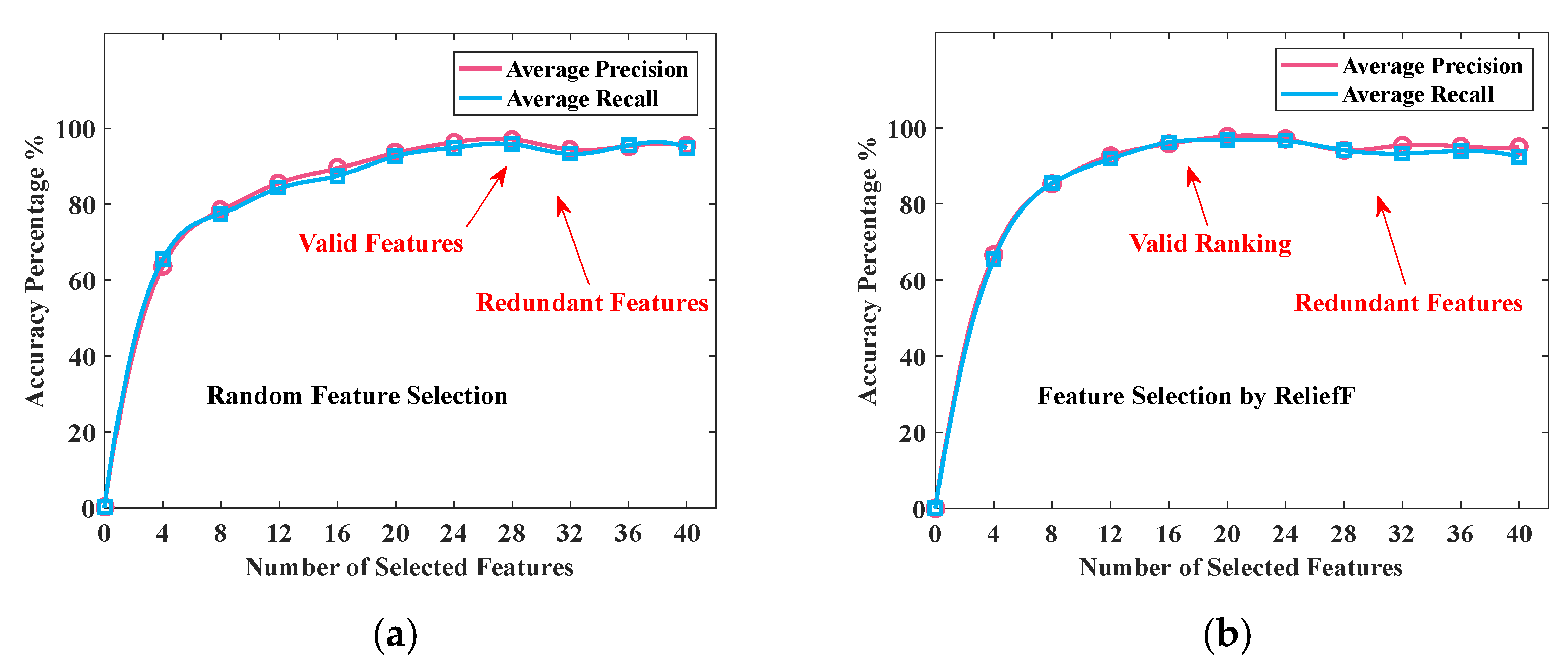
5.3. ReliefF Feature Selection

As an optimal feature selection approach, the ReliefF algorithm was adopted to achieve dimension reduction for the original feature vectors. The embedded dimension parameter of the permutation entropy was set to six in this case. The permutation entropy’s time delay parameter was set as one. The permutation entropy hard barrier was set to 0.6.

Two feature selection methods, random feature selection and ReliefF algorithm, were used for comparison. Figure 13a,b present the precision and recall results through random feature selection and ReliefF algorithm, respectively. All the accuracy trends rise with the feature number increasing at the early stage. This is because the first selected features would help to train the classifier model directly. In Figure 13a, the random feature selection algorithm obtains the highest accuracy when selecting 22 top-ranked features. At this time, the average precision and average recall ratio reached 97.3 percent and 96.5 percent, respectively. As a comparison, in Figure 13b, the ReliefF feature selection algorithm obtains the highest accuracy when selecting 17 top-ranked features. Meanwhile, the average precision and average recall ratio achieved by ReliefF reached 98.2 percent and 97.9 percent, respectively. The reason for the rising accuracy is easy to understand. When the feature number is small, the classifier model lacks training. Hence, increasing features would help to construct the classification hyperplane for SVM models.

Nevertheless, after the best-feature dimension, both classifier models drop in accuracies due to the redundant features involved. After decreasing, the precision and the recall values rise a little again. The reason for this is that we selected the RBF as the SVM kernel. The slack variable and the penalty parameters import soft intervals, which contribute to building a decision boundary under a tolerant error. The soft interval boundary improves the robustness and generalization of SVM models.

Then, the classifier accuracy is tested under different ratios of training sets to further investigate the effectiveness and robustness of the feature selection procedure. The training set’s percentages were increased by 10 percent, 20 percent, 30 percent, 40 percent, 50 percent, and 60 percent, respectively. For each training set percentage, 1000 trials were performed to reduce random effects. Figure 14a,b presents the average accuracy bar graph for different percentages of verification and testing datasets. In the figures, the error standard deviations are also indicated. To be specific, 22 top-ranked features were chosen for training and testing by random feature selection, which is shown in Figure 14a. Meanwhile, 17 top-ranked features were chosen for training and testing by the ReliefF algorithm, as shown in Figure 14b.

Overall, it was observed that both training and testing accuracies with the optimal selection perform better than the randomly selected results. In Figure 14a,b, the training accuracy was greater than the testing accuracy when the training percentage was only 10%. This indicates that the classifier is underfitting. Then, the accuracy for test sets rises with the increasing percentage for training sets. It is understandable that the classifier is well trained, with increasing training samples for both optimal selection and random selection. When the training percentage increased to 60%, the training and testing accuracies were closed by the ReliefF selection algorithm in Figure 14a. Moreover, the accuracy error between verification and test results decreased gradually for ReliefF selection. To be specific, when the training percentage was 10%, 20%, 30%, 40%, 50%, and 60%, the average accuracy difference between verification and test was 1.8%,1.4%, 1.6%, 0.8%, 0.6%, and 0.3%, respectively. However, for random feature selection in Figure 14b, the error between the verification and test accuracy was not reduced with an increasing training percentage. The average accuracy difference between verification and test was 4.1%, 2.7%, 2.3%, 1.8%, 1.7%, and 1.9%. Comparing the average accuracy difference between verification and test, it was found that the accuracy of the ReliefF algorithm was always better than random selection, even on the same training percentage. As referred to above, for each training set percentage, 1000 trials were performed to reduce random effects. Therefore, each training result varies, and the error results are marked in a black line on the bar. For a specific training percentage, the error bar shows that the accuracy error by ReliefF is much smaller than random selection. For instance, the verification accuracy error by ReliefF is 0.83%, 0.72%, 0.70%, 0.65%, 0.59%, and 0.48% when the training percentage is 10%, 20%, 30%, 40%, 50%, and 60%, respectively. However, the verification accuracy error by random selection is 0.93%, 0.90%, 0.91%, 0.92%, 0.90%, and 0.94% when the training percentage is 10%, 20%, 30%, 40%, 50%, and 60%. Obviously, the error does not decrease, which also shows that the randomly selected classifier is less robust than ReliefF. Based on this comparison, it was verified the constructed model by random selection is always underfitting. In other words, the randomly selected features are not optimal for the classifier model. Therefore, it is essential to perform the feature selection procedure before constructing the classifier model.

5.4. Performance with Real Experiments

To present the results of the proposed algorithm, the following indicators [30] were used as follows: precision for correctly recognizing the PQD event, defined as P_event; recall for correctly recognizing the PQD event, R_event; precision for incorrectly recognizing the PQD event, defined as P_others; and recall for incorrectly recognizing the PQD event, defined as R_others.

$$\begin{array}{l}{P}_{\mathrm{event}}=\frac{TP}{TP+FP}\\ R_{\mathrm{event}}=\frac{TP}{TP+FN}\\ P_{\mathrm{others}}=\frac{TN}{TN+FN}\\ R_{\mathrm{others}}=\frac{FP}{FP+TN}\\ A\mathrm{ccuracy}=\frac{TP+TN}{TP+FP+TN+FN}\times 100\%\end{array}$$

(19)

In Equation (20), the parameter TP denotes the example number for true positive, which represents that the predicted PQD event was truly recognized. The parameter FP stands for the example number of false positives, which signifies that another PQD was mistakenly identified as the anticipated PQD event. The number of false-negative instances represents the number of times the estimated PQD event was mistakenly identified as another PQD event. TN stands for true negative occurrences, which indicates that another PQD type was correctly identified as the associated PQD event [31]. The confusion matrix is imported to exhibit the PQD classification results, and the validation datasets are shown in

Table 3. Confusion matrix of the classification results.

Assigned Class	True Class
	C1	C2	C3	C4	C5	C6	C7	C8	C9	C10
C1	423	0	0	0	0	0	0	0	0	0
C2	0	435	0	0	0	0	0	0	0	0
C3	1	0	406	0	0	0	0	0	0	0
C4	0	3	0	411	0	0	0	0	0	0
C5	0	0	0	0	428	0	0	0	0	0
C6	0	0	0	0	0	403	0	0	0	0
C7	0	0	0	0	0	0	415	0	0	0
C8	0	0	0	0	0	0	0	437	0	0
C9	0	0	0	0	0	0	0	0	429	0
C10	0	0	0	0	0	0	0	0	2	422

.

The confusion matrix verifies that the classification results achieved high accuracy. Unfortunately, some samples were assigned to incorrect classes. For instance, one C3 (Swell) case was incorrectly recognized as C1 (pure sine). This was because a swelling event occurred less than 3 T. The amplitude parameter α was also close to 0.1. Additionally, three C4 (interrupt) cases were recognized as C2 (sag). As seen in the PQD mathematical model, the definitions of C4 and C2 are the same. The only difference is the value selection for the parameter α.

5.5. Performance with Noisy Data

Table 4. Classification accuracy performance in a noisy environment.

Recognized Class	Signal-to-Noise Ratio
	15 dB	25 dB	35 dB
C1	95.2%	99.2%	100%
C2	100%	100%	100%
C3	98.2%	100%	100%
C4	100%	100%	100%
C5	95.2%	96.8%	98.0%
C6	96.4%	98.2%	100%
C7	93.8%	97.4%	98.2%
C8	98.2%	98.8%	100%
C9	100%	100%	100%
C10	97.6%	98.2%	99.2%
Overall	97.41%	98.86%	99.54%

illustrates the proposed classifier’s performance at 15 dB, 25 dB, and 35 dB SNRs for 500 test samples. As can be observed from the table, the accuracy results verify that the proposed model exhibits excellent noise tolerance in the dataset. The number of PQDs and the corresponding event types were chosen at random from the training dataset. As can be observed from Table 4, the classification accuracy improved with the SNR’s increase. Clearly, the classifier performs more admirably in a less-noisy environment on a 35 dB SNR. Moreover, the test results reveal that the developed method was less sensitive to noise in the practical environment. For instance, the lowest accuracy was achieved at 93.8% at C7 classes under 15dB SNR. This might be credited to the EWT algorithm’s good performance, which uses empirical wavelet filters to divide signals into independent components in frequency spectrums. The signal’s effective elements with noisy disturbance are then extracted. The feature extraction approach that follows is also beneficial to EWT decomposition.

6. Conclusions

This paper presents a practical method for PQD event recognition. By using empirical wavelet transform and optimized parameters, the obtained signal is transformed into several intrinsic mode function components. After, the statistical features are extracted from the decomposed subcomponents. Then, the feature selection algorithm, ReliefF, is adopted to reconstruct the optimal feature vectors. Finally, the improved feature vectors are loaded into a multiclass SVM model to identify various PQD event instances. To test the effectiveness of the proposed algorithm, a simulation dataset, as well as a real dataset on the microgrid platform, was used for several experimental investigations. By using the ReliefF algorithm, 17 top-ranked features were valid for reconstruction. The final classification accuracy achieved 97.41%, 98.86%, and 99.54% when the SNR is 15 dB, 25 dB, and 35 dB, respectively. The main conclusions of this work are summarized as follows. Compared with the EMD, the EWT is more adaptive and robust in signal segmentation and denoising. Feature selection techniques, such as the ReliefF algorithm, are effective and essential in filtering the significant components and eliminating redundant features. After selection, both the accuracy and the computing efficiency improved when the prominent features were identified. Based on the performance analysis, the proposed method demonstrates significant adaptability in various noisy situations, whether for PQD detection sensitivity or specificity.

References

1. Xiao, F.; Ai, Q. Data-Driven Multi-Hidden Markov Model-Based Power Quality Disturbance Prediction That Incorporates Weather Conditions. IEEE Trans. Power Syst. 2019, 34, 402–412. [Google Scholar] [CrossRef]
2. Xiao, F.; Lu, T.; Ai, Q.; Wang, X.; Chen, X.; Fang, S.; Wu, Q. Design and Implementation of a Data-Driven Approach to Visualizing Power Quality. IEEE Trans. Smart Grid 2020, 11, 4366–4379. [Google Scholar] [CrossRef]
3. Jena, M.K.; Panigrahi, B.K.; Samantaray, S.R. A New Approach to Power System Disturbance Assessment Using Wide-Area Postdisturbance Records. IEEE Trans. Ind. Inform. 2018, 14, 1253–1261. [Google Scholar] [CrossRef]
4. Liang, C.; Teng, Z.; Li, J.; Yao, W.; Hu, S.; Yang, Y.; He, Q. A Kaiser Window-Based S-Transform for Time-Frequency Analysis of Power Quality Signals. IEEE Trans. Ind. Inform. 2021, 18, 965–975. [Google Scholar] [CrossRef]
5. Gu, T.Y.; Gao, Y.P.; Wu, C.; Lin, C.H.; Fan, Q.; Xu, M.M. Power quality disturbance detection based on improved wavelet threshold function and singular value decomposition. Electr. Meas. Instrum. 2020, 57, 111–118. [Google Scholar]
6. Solis-Munoz, F.J.; Elvira-Ortiz, D.A.; Jaen-Cuellar, A.Y.; Romero-Troncoso, R.; Osornio-Rios, R.A. A Novel Methodology for Power Quality Disturbances Detection and Classification in Industrial Facilities. J. Sci. Ind. Res. 2020, 79, 819–823. [Google Scholar]
7. Mahela, O.P.; Khan, B.; Alhelou, H.H.; Tanwar, S. Assessment of power quality in the utility grid integrated with wind energy generation. IET Power Electron. 2020, 13, 2917–2925. [Google Scholar] [CrossRef]
8. He, S.; Li, K.; Zhang, M. A Real-Time Power Quality Disturbances Classification Using Hybrid Method Based on S-Transform and Dynamics. IEEE Trans. Instrum. Meas. 2013, 62, 2465–2475. [Google Scholar] [CrossRef]
9. Abdelsalam, A.A.; Hassanin, A.M.; Hasanien, H.M. Categorisation of power quality problems using long short-term memory networks. IET Gener. Transm. Distrib. 2021, 15, 1626–1639. [Google Scholar] [CrossRef]
10. Om Prakash, M.; Abdul Gafoor, S. Power quality recognition in distribution system with solar energy penetration using S-transform and Fuzzy C-means clustering. Renew. Energy 2017, 106, 37–51. [Google Scholar]
11. Yu, Y.; Zhao, W.; Li, S.; Huang, S. A Two-Stage Wavelet Decomposition Method for Instantaneous Power Quality Indices Estimation Considering Interharmonics and Transient Disturbances. IEEE Trans. Instrum. Meas. 2021, 70, 1–13. [Google Scholar] [CrossRef]
12. Choe, S.; Yoo, J. Wavelet Packet Transform Modulus-Based Feature Detection of Stochastic Power Quality Disturbance Signals. Appl. Sci. 2021, 11, 2825. [Google Scholar] [CrossRef]
13. Manjula, M.; Mishra, S.; Sarma, A. Empirical mode decomposition with Hilbert transform for classification of voltage sag causes using probabilistic neural network. Int. J. Electr. Power Energy Syst. 2013, 44, 597–603. [Google Scholar] [CrossRef]
14. Singh, R.H.; Mohanty, S.R.; Kishor, N.; Thakur, K.A. Real-Time Implementation of Signal Processing Techniques for Dis-turbances Detection. Electr. Power Syst. Res. 2019, 66, 3550–3560. [Google Scholar]
15. Gilles, J. Empirical wavelet transform. IEEE Trans. Signal. Process. 2013, 61, 3999–4010. [Google Scholar] [CrossRef]
16. Kamble, S.; Thote, P.; Rathore, C.; Marothiya, A. Estimation of various PQ indices at point of common coupling using empirical wavelet transform. IET Sci. Meas. Technol. 2019, 13, 862–873. [Google Scholar] [CrossRef]
17. Thirumala, K.; Umarikar, A.C.; Jain, T. Estimation of Single-Phase and Three-Phase Power-Quality Indices Using Empirical Wavelet Transform. IEEE Trans. Power Deliv. 2014, 30, 445–454. [Google Scholar] [CrossRef]
18. Fu, L.; Zhu, T.; Pan, G.B.; Chen, S.H.; Zhong, Q.; Wei, Y.D. Power Quality Disturbance Recognition Using VMD-Based Feature Extraction and Heuristic Feature Selection. Appl. Sci. 2019, 9, 4901. [Google Scholar] [CrossRef] [Green Version]
19. Chaudhary, P.; Rizwan, M. Voltage regulation mitigation techniques in distribution system with high PV penetration: A review. Renew. Sustain. Energy Rev. 2018, 82, 3279–3287. [Google Scholar] [CrossRef]
20. Naderian, S.; Salemnia, A. Method for classification of PQ events based on discrete Gabor transform with FIR window and T2FK-based SVM and its experimental verification. IET Gener. Transm. Distrib. 2017, 11, 133–141. [Google Scholar] [CrossRef]
21. Liu, Z.; Cui, Y.; Li, W. A Classification Method for Complex Power Quality Disturbances Using EEMD and Rank Wavelet SVM. IEEE Trans. Smart Grid 2015, 6, 1678–1685. [Google Scholar] [CrossRef]
22. Achlerkar, P.D.; Samantaray, S.; Manikandan, M.S. Variational Mode Decomposition and Decision Tree Based Detection and Classification of Power Quality Disturbances in Grid-Connected Distributed Generation System. IEEE Trans. Smart Grid 2016, 9, 3122–3132. [Google Scholar] [CrossRef]
23. Xi, Y.; Li, Z.; Tang, X.; Zeng, X. Classification of power quality disturbances based on KF-ML-aided S-transform and multilayers feedforward neural networks. IET Gener. Transm. Distrib. 2020, 14, 4010–4020. [Google Scholar] [CrossRef]
24. Fu, L.; Wei, Y.; Fang, S.; Zhou, X.; Lou, J. Condition Monitoring for Roller Bearings of Wind Turbines Based on Health Evaluation under Variable Operating States. Energies 2017, 10, 1564. [Google Scholar] [CrossRef] [Green Version]
25. Xie, S.; Li, K.; Xiao, M.; Zhang, L.; Li, W. Key Quality Indicators Prediction for Web Browsing with Embedded Filter Feature Selection. Appl. Sci. 2020, 10, 2141. [Google Scholar] [CrossRef] [Green Version]
26. IEEE. 1159-1995 IEEE Recommended Practice for Monitoring Electric Power Quality. 1995, pp. 1–80. Available online: https://webstore.ansi.org/standards/ieee/11591995 (accessed on 1 December 2021).
27. Khokhar, S.; Zin, A.A.M.; Memon, A.P.; Mokhtar, A.S. A new optimal feature selection algorithm for classification of power quality disturbances using discrete wavelet transform and probabilistic neural network. Measurements 2017, 95, 246–259. [Google Scholar] [CrossRef]
28. Fu, L.; Zhu, T.; Zhu, K.; Yang, Y. Condition Monitoring for the Roller Bearings of Wind Turbines under Variable Working Conditions Based on the Fisher Score and Permutation Entropy. Energies 2019, 12, 3085. [Google Scholar] [CrossRef] [Green Version]
29. Thirumala, K.; Pal, S.; Jain, T.; Umarikar, A.C. A classification method for multiple power quality disturbances using EWT based adaptive filtering and multiclass SVM. Neurocomputing 2019, 334, 265–274. [Google Scholar] [CrossRef]
30. Zhu, T.; Qu, Z.; Xu, H.; Zhang, J.; Shao, Z.; Chen, Y.; Prabhakar, S.; Yang, J. RiskCog: Unobtrusive Real-Time User Authentication on Mobile Devices in the Wild. IEEE Trans. Mob. Comput. 2020, 19, 466–483. [Google Scholar] [CrossRef]
31. Zhu, T.; Fu, L.; Liu, Q.; Lin, Z.; Chen, Y.; Chen, T. One Cycle Attack: Fool Sensor-Based Personal Gait Authentication with Clustering. IEEE Trans. Inf. Forensics Secur. 2021, 16, 553–568. [Google Scholar] [CrossRef]
Figure 1. EWT partitioning of the Fourier spectrum axis.
Electronics 11 00174 g001
Figure 2. Main flowchart of the proposed method.
Electronics 11 00174 g002
Figure 3. The waveform of 10 representative PQD signals.
Electronics 11 00174 g003
Figure 4. Experimental platform for electronic system simulation.
Electronics 11 00174 g004
Figure 5. Original sag with harmonics signal.
Electronics 11 00174 g005
Figure 6. PQD signal decomposition results by EWT when K = 4. (a) Results in the time domain; (b) Segmented spectrum.
Electronics 11 00174 g006
Figure 7. PQD signal decomposition results by EWT when K = 5. (a) Results in the time domain; (b) Segmented spectrum.
Electronics 11 00174 g007
Figure 8. PQD signal decomposition results by EWT when K = 6. (a) Results in the time domain; (b) Segmented spectrum.
Electronics 11 00174 g008
Figure 9. PQD signal decomposition results by EWT when K = 8. (a) Results in the time domain; (b) Segmented spectrum.
Electronics 11 00174 g009
Figure 10. Decomposition results in time domain by EMD.
Electronics 11 00174 g010
Figure 11. Swell with harmonics decomposition results by EWT when K = 8. (a) Results in the time domain; (b) Results in the frequency domain.
Electronics 11 00174 g011
Figure 12. Periodic notch decomposition results by EWT when K = 8. (a) Results in the time domain; (b) Results in the frequency domain.
Electronics 11 00174 g012
Figure 13. Recognition accuracy under different selected features. (a) Training result by random selection; (b) Training result by ReliefF selection.
Electronics 11 00174 g013
Figure 14. Accuracy comparison with different training percentages. (a) Accuracy with feature selection; (b) Accuracy without feature selection.
Electronics 11 00174 g014