
Cooperative Multi-Node Jamming Recognition Method Based on Deep Residual Network
Abstract
:1. Introduction
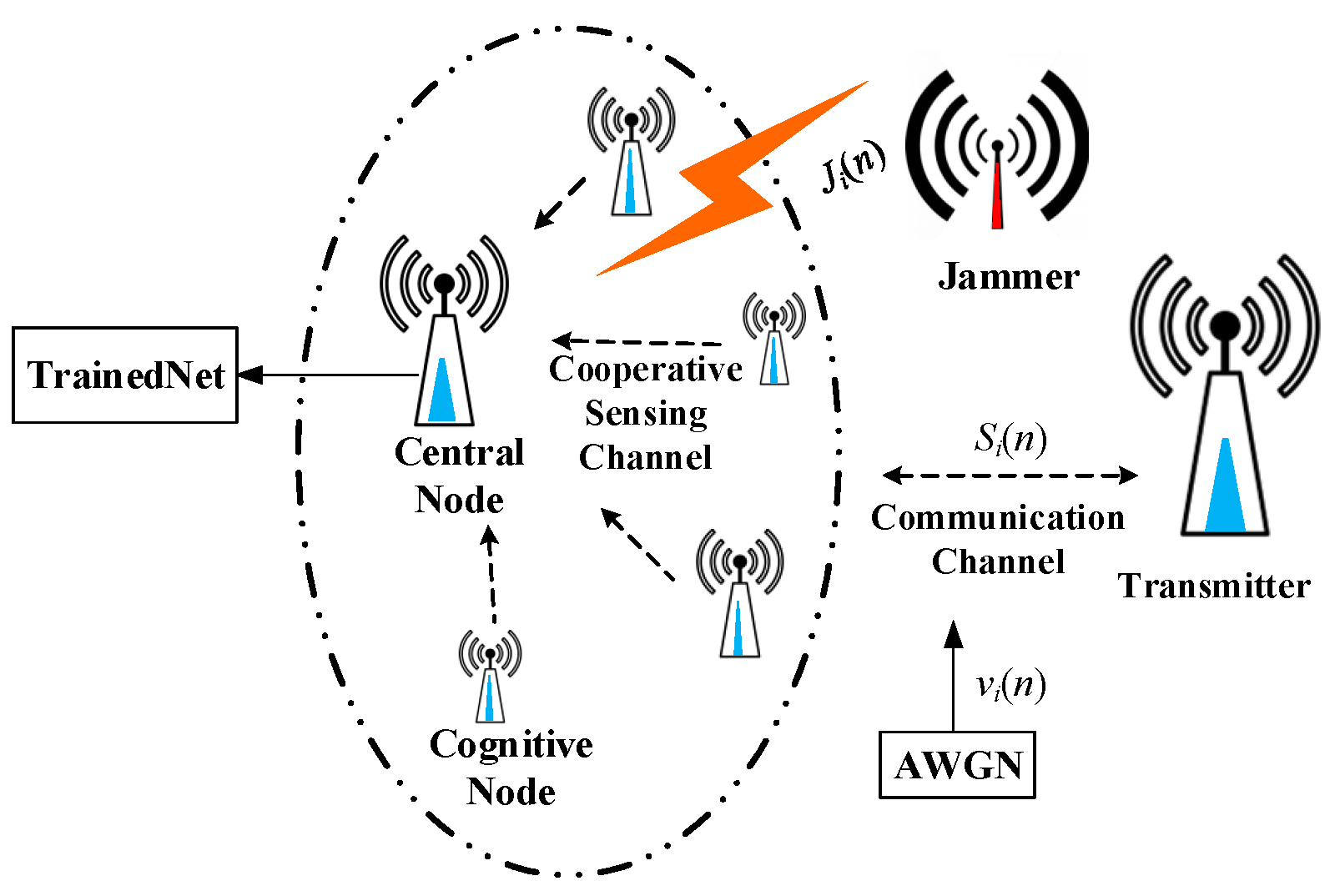
2. System Model
3. Cooperative Multi-Node Jamming Recognition Method Based on Deep Residual Network
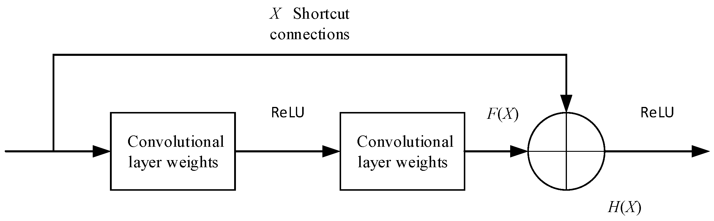
3.1. Residual Connections
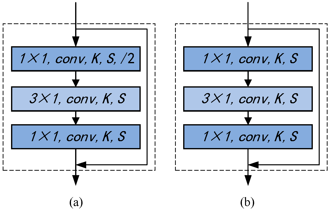
3.2. Residual Network Structure
3.3. Multi-Node Cooperative Jamming Recognition Method
4. Simulation Result and Analysis
4.1. Parameter Settings
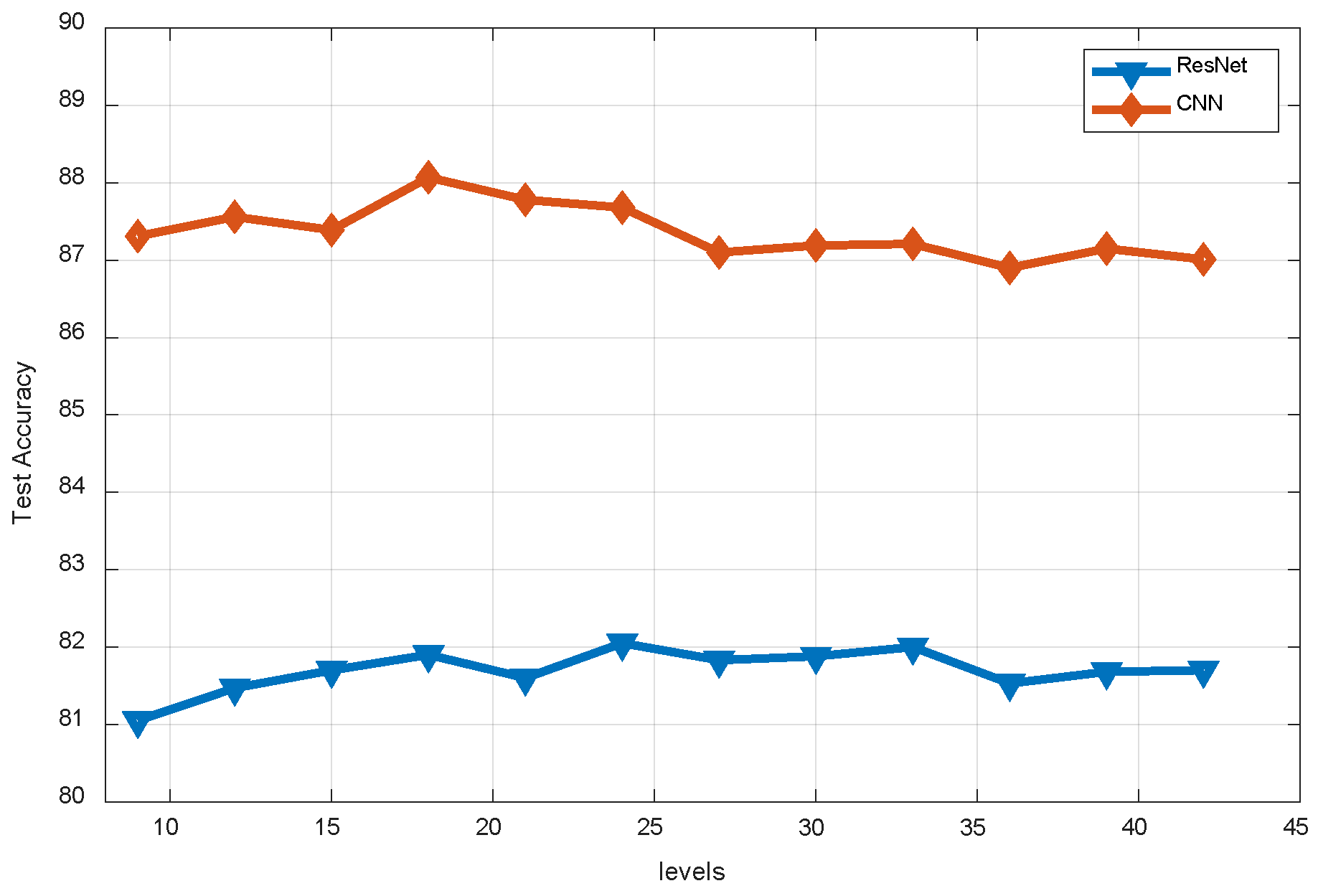
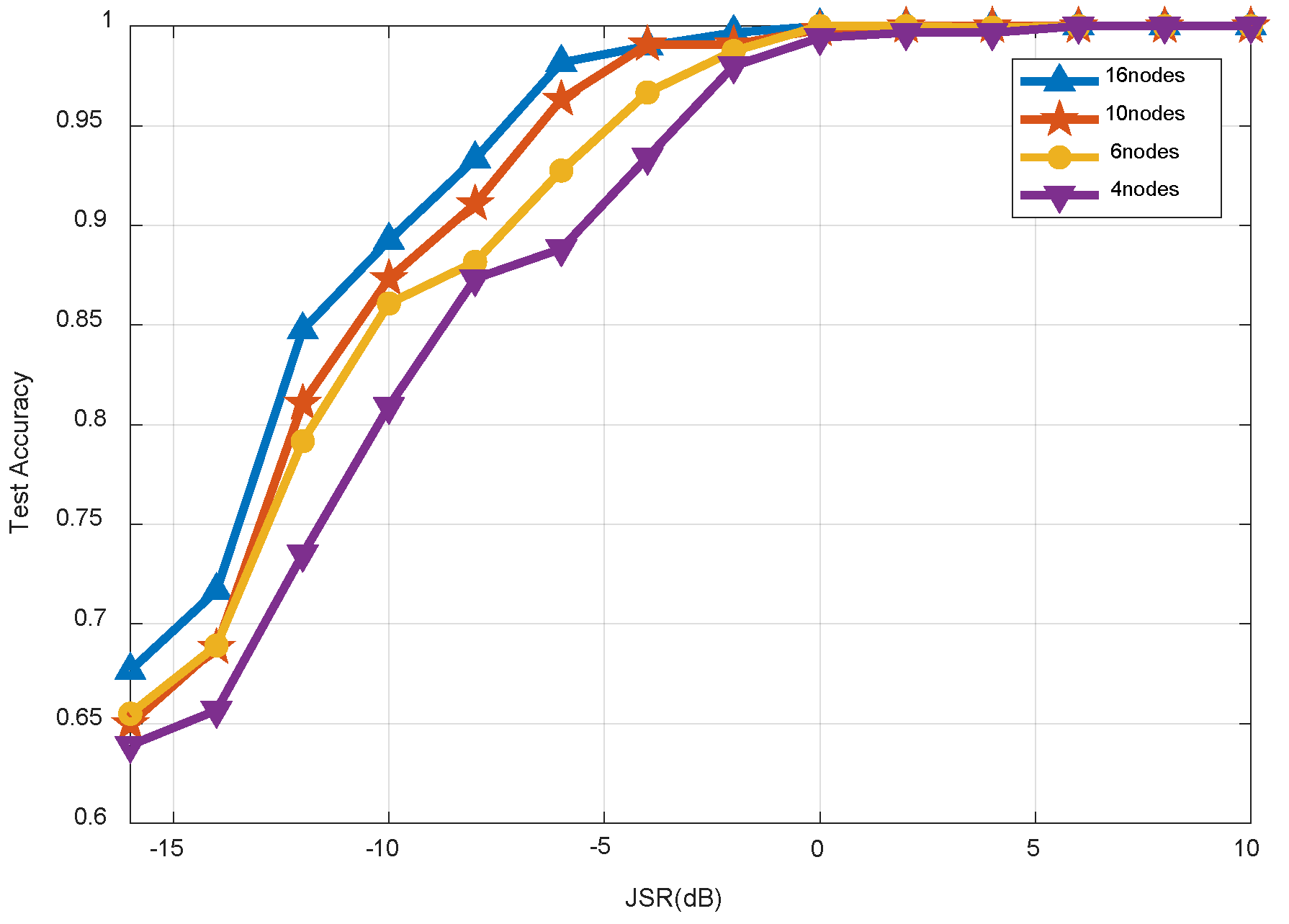
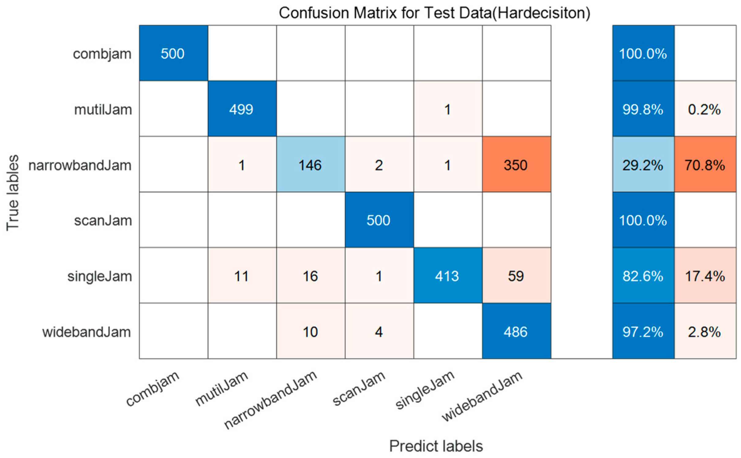
4.2. Performance Analysis
5. Conclusions
Author Contributions
Funding
Conflicts of Interest
References
- Yao, F. Communication Anti-Interference Engineering and Practice; Electronic Industry Press: Beijing, China, 2012. [Google Scholar]
- Lang, B.; Gong, J. JR-TFViT: A Lightweight Efficient Radar Jamming Recognition Network Based on Global Representation of the Time–Frequency Domain. Electronics 2022, 11, 2794. [Google Scholar] [CrossRef]
- Choi, H.; Park, S.; Lee, H. Covert Anti-Jamming Communication Based on Gaussian Coded Modulation. Appl. Sci. 2021, 11, 3759. [Google Scholar] [CrossRef]
- Jia, L.; Xu, Y.; Sun, Y.; Feng, S.; Anpalagan, A. Stackelberg game approaches for anti-jamming defence in wireless networks. IEEE Wirel. Commun. 2018, 25, 120–128. [Google Scholar] [CrossRef] [Green Version]
- Xuan, Y.; Shen, Y.; Shin, I.; Thai, M.T. On Trigger Detection against Reactive Jamming Attacks: A Clique-Independent Set Based Approach. In Proceedings of the PERFORMANCE Computing and Communications Conference, Scottsdale, AZ, USA, 14–16 December 2009; pp. 223–230. [Google Scholar]
- Yang, X.; Ruan, H. A Recognition Method of Deception Jamming Based on image Zernike Moment Feature of Time-frequency Distribution. Mod. Radar 2018, 40, 91–95. [Google Scholar]
- Fang, F.; Li, Y.; Niu, Y. Jamming signal recognition based on decision tree algorithm. Commun. Technol. 2019, 52, 2617–2623. [Google Scholar]
- Julian, W.; Kazuto, Y.; Norisato, S.; Yafei, H.; Eiji, N.; Toshihide, H.; Abolfazl, M.; Yoshinori, S. WLAN Interference Identification Using a Convolutional Neural Network for Factory Environments. J. Commun. 2021, 16, 276–283. [Google Scholar]
- Lan, X.; Wan, T.; Jiang, K.; Xiong, Y.; Tang, B. Intelligent Recognition of Chirp Radar Deceptive Jamming Based on Multi-Pulse Information Fusion. Sensors 2021, 21, 2693. [Google Scholar] [CrossRef]
- Zhou, H.; Dong, C.; Wu, R.; Xu, X.; Guo, Z. Feature Fusion Based on Bayesian Decision Theory for Radar Deception Jamming Recognition. IEEE Access 2021, 9, 16296–16304. [Google Scholar] [CrossRef]
- Yu, C.; Zhao, M.; Song, M.; Wang, Y.; Li, F.; Han, R.; Chang, C.-I. Hyperspectral image classification method based on CNN Architecture embedding with hashing semantic feature. IEEE J. Sel. Top. Appl. Earth Obs. Remote Sens. 2019, 12, 1866–1881. [Google Scholar] [CrossRef]
- Lu, S.; Meng, Z.; Huang, J.; Yi, M.; Wang, Z. Study on Quantum Radar Detection Probability Based on Flying-Wing Stealth Aircraft. Sensors 2022, 22, 5944. [Google Scholar] [CrossRef] [PubMed]
- Cheng, D.; Fan, Y.; Fang, S.; Wang, M.; Liu, H. ResNet-AE for Radar Signal Anomaly Detection. Sensors 2022, 22, 6249. [Google Scholar] [CrossRef]
- Malik, M.; Magaña-Loaiza, O.S.; Robert, W.B. Quantum-secured imaging. Appl. Phys. Lett. 2012, 101, 241103. [Google Scholar] [CrossRef] [Green Version]
- You, S.; Diao, M.; Gao, L. Implementation of a combinatorial-optimisation-based threat evaluation and jamming allocation system. IET Radar Sonar. Navig. 2019, 13, 1636–1645. [Google Scholar] [CrossRef]
- Zhao, S.; Yi, M.; Liu, Z. Cooperative Anti-Deception Jamming in a Distributed Multiple-Radar System under Registration Errors. Sensors 2022, 22, 7216. [Google Scholar] [CrossRef]
- Shen, J.; Li, Y.; Shi, Y.; An, K. Multi-node Cooperative Jamming Recognition Method Based on Deep Convolutional Neural Network. Radio Commun. Technol. 2022, 48, 711–717. [Google Scholar]
- Zhao, Y.; Zhang, X.; Feng, W.; Xu, J. Deep Learning Classification by ResNet-18 Based on the Real Spectral Dataset from Multispectral Remote Sensing Images. Remote Sens. 2022, 14, 4883. [Google Scholar] [CrossRef]
- Li, X.-X.; Li, D.; Ren, W.-X.; Zhang, J.-S. Loosening Identification of Multi-Bolt Connections Based on Wavelet Transform and ResNet-50 Convolutional Neural Network. Sensors 2022, 22, 6825. [Google Scholar] [CrossRef] [PubMed]
- He, K.; Zhang, X.; Ren, S.; Sun, J. Deep residual learning for image recognition. In Proceedings of the IEEE Conference on Computer Vision and Pattern Recognition, Las Vegas, NV, USA, 27–30 June 2016; pp. 770–778. [Google Scholar]
- Nair, R.G.; Narayanan, K. Cooperative spectrum sensing in cognitive radio networks using machine learning techniques. Appl. Nanosci. 2022. [Google Scholar] [CrossRef]
- Sarikhani, R.; Keynia, F. Cooperative Spectrum Sensing Meets Machine Learning: Deep Reinforcement Learning Approach. IEEE Commun. Lett. 2020, 24, 1459–1462. [Google Scholar] [CrossRef]
- Xie, J.; Fang, J.; Liu, C.; Li, X. Deep Learning-Based Spectrum Sensing in Cognitive Radio: A CNN-LSTM Approach. IEEE Commun. Lett. 2020, 24, 2196–2200. [Google Scholar] [CrossRef]
- Zhou, F.; Beaulieu, N.; Li, Z.; Si, J. Feasibility ofmaximum eigenvalue cooperative spectrum sensing based on Cholesky factorisation. IET Commun. 2016, 10, 199–206. [Google Scholar] [CrossRef]
- Thilina, K.; Choi, K.; Saquib, N.; Hossain, E. Machinelearning techniques for cooperative spectrum sensing incognitive radio networks. IEEE J. Sel. Areas Commun. 2013, 31, 2209–2221. [Google Scholar] [CrossRef]
- Liu, X.; Yang, D.; Gamal, A. Deep Neural Network Architectures for Modulation classification. In Proceedings of the 2017 51st Asilomar Conference on Signals, Systems, and Computers, Pacific Grove, CA, USA, 29 October 2017–1 November 2017. [Google Scholar]
- Niu, Y.; Yao, F.; Chen, J. Fuzzy Jamming Pattern Recognition Based on Statistic Parameters of Signal’s PSD. J. China Ordnance 2011, 7, 15–23. [Google Scholar]
- Gai, J.; Xue, X.; Wu, J. Cooperative Spectrum Sensing Method Based on Deep Convolutional Neural Network. J. Electron. Inf. 2021, 43, 2911–2919. [Google Scholar]
- Valadão, M.; Amoedo, D.; Costa, A.; Carvalho, C.; Sabino, W. Deep Cooperative Spectrum Sensing Based on Residual Neural Network Using Feature Extraction and Random Forest Classifier. Sensors 2021, 21, 7146. [Google Scholar] [CrossRef] [PubMed]
- Janu, D.; Singh, K.; Kumar, S. Machine learning for cooperative spectrum sensing and sharing: A survey. Trans. Emerg. Telecommun. Technol. 2021, 33, e4352. [Google Scholar] [CrossRef]
- Woongsup, L.; Minhoe, K.; Dong-Ho, C. Deep Cooperative Sensing: Cooperative Spectrum Sensing Based on Convolutional Neural Networks. IEEE Trans. Veh. Technol. 2019, 68, 3005–3009. [Google Scholar]


| Index | Layers | Output Dimension |
|---|---|---|
| 1 | Input | 512 × 1 |
| 2 | 15 × 1,conv,48 | 512 × 1 |
| 3 | 7 × 1,conv,64 | 512 × 1 |
| 4 | 3 × 1,maxpool,/2 | 256 × 1 |
| 5 | Residual-block1 (64) | 128 × 1 |
| 6 | Residual-block2 (64) | 128 × 1 |
| 7 | Residual-block1 (128) | 64 × 1 |
| 8 | Residual-block2 (128) | 64 × 1 |
| 9 | Residual-block2 (128) | 64 × 1 |
| 10 | 32 × 1,average pooling layer | 1 × 256 |
| 11 | fc × 32 | 1 × 32 |
| 12 | Softmax, fc × 6 | 1 × 6 |
| Training Parameters | Numerical Values |
|---|---|
| Initial learning rate | 0.001 |
| Number of iterative rounds | 6 |
| Small batch size | 128 |
| Parameter optimizer | Adam |
| Learning rate drop period | 9 |
| Convolution kernel size Desampling step size | 1 × 1, 3 × 1, 7 × 1, 15 × 1 2 |
| Input: sensory information from M co-cognitive nodes Output: global jamming signal classification judgement |
| Step 1: (Training phase) The central node trains a neural network “Trainednet” using the perceptual information of the M co-cognitive nodes and distributes the network parameters to each co-cognitive node. |
| Step 2: (Testing phase) The M co-cognitive nodes use the trained neural network to perform classification judgments, independently obtain recognition results Hi and send the recognition results back to the central node. |
| Step 3: (Data fusion phase) The central node performs data fusion based on the sensory information of each cooperative cognitive node and derives the global recognition result Hw based on the majority judgment criterion, which is used as the final recognition result of the multi-node cooperative jamming recognition network. |
| Input: sensory information from M co-cognitive nodes Output: global jamming signal classification judgement |
| Step 1: (Training phase) The central node trains a neural network “Trainednet” using the sensory information of the M co-cognitive nodes and distributes the network parameters to each co-cognitive node. |
| Step 2: (Testing phase) The M co-cognitive nodes use the trained neural network to perform classification judgments, obtain recognition vectors Vi independently and transmit the recognition results back to the central node. |
| Step 3: (Data fusion phase) The central node performs data fusion based on the sensory information of each cooperative cognitive node, all vectors are added to obtain the global judgment vector Vw, and the jamming with the highest probability is used as the global recognition result Hw. |
| Jamming Pattern | Jamming Parameters |
|---|---|
| Single-tone Jamming | The frequency point is randomly located near the carrier frequency fc. |
| Multi-tone Jamming | The frequency point is randomly located near the carrier frequency fc. The number of tones is random. |
| Narrow-band Jamming | The central frequency is located at fc and the band width is randomly generated. |
| Broad-band Jamming | The central frequency is located at fc and the band width is randomly generated. |
| Comb Jamming | Initial frequency is random around fc and the number and intervals of frequency points are random. |
| Sweep Jamming | Initial frequency is random around fc. |
| Net | Average Correct Recognition Rate |
|---|---|
| ResNet | 88.08% |
| CNN (Lenet) | 82.41% |
Publisher’s Note: MDPI stays neutral with regard to jurisdictional claims in published maps and institutional affiliations. |
© 2022 by the authors. Licensee MDPI, Basel, Switzerland. This article is an open access article distributed under the terms and conditions of the Creative Commons Attribution (CC BY) license (https://creativecommons.org/licenses/by/4.0/).
Share and Cite
Shen, J.; Li, Y.; Zhu, Y.; Wan, L. Cooperative Multi-Node Jamming Recognition Method Based on Deep Residual Network. Electronics 2022, 11, 3280. https://doi.org/10.3390/electronics11203280
Shen J, Li Y, Zhu Y, Wan L. Cooperative Multi-Node Jamming Recognition Method Based on Deep Residual Network. Electronics. 2022; 11(20):3280. https://doi.org/10.3390/electronics11203280
Chicago/Turabian StyleShen, Junren, Yusheng Li, Yonggang Zhu, and Liujin Wan. 2022. "Cooperative Multi-Node Jamming Recognition Method Based on Deep Residual Network" Electronics 11, no. 20: 3280. https://doi.org/10.3390/electronics11203280