Efficient Microwave Filter Design by a Surrogate-Model-Assisted Decomposition-Based Multi-Objective Evolutionary Algorithm

Abstract

As a crucial frequency selection device in modern communication systems, the microwave filter plays an increasingly prominent role. There is a great demand for the multi-objective design of microwave filters. The filter’s performance affects the quality of the whole communication system directly. However, traditional multi-objective electromagnetic (EM) optimization design demands repetitive EM simulations to adjust the physical parameters of the microwave filters. Accordingly, using electromagnetic simulation directly to design optimization is quite expensive. Given this situation, this paper applies a novel surrogate model based on one-dimensional convolutional autoencoders (1D-CAE) into the multi-objective algorithm evolutionarily based on decomposition (MOEA/D) for the first time. This approach uses MOEA/D as the multi-objective optimizer, and a novel low-complexity surrogate model based on one-dimensional convolutional autoencoders (1D-CAE) is constructed to predict the expensive EM simulation results. The surrogate model based on 1D-CAE is used to generate the results of scalar subproblems of MOEA/D, which greatly improves the design efficiency. Compared with the traditional design methods based on an EM solver, this method not only effectively optimizes multiple design objectives but also completes the design of microwave filters in a shorter time. The proposed method is verified using the design of a sixth-order ceramic filter and a seventh-order metal cavity filter.

1. Introduction

The microwave filter is quite a vital RF device in wireless communication systems. With the rapid development of wireless communication technology, it is very important to improve the efficiency of filter design. In recent years, a variety of optimization algorithms, such as particle swarm optimization (PSO), ant colony optimization (ACO), and differential evolution (DE), are receiving widespread attention. PSO, ACO, DE, and population-based incremental learning (PBIL) have gained recognition in filter design [1,2,3,4,5,6]. However, in the design process of microwave filters, engineers cannot just consider a single design objective but need to achieve equilibrium among multiple different objectives, so as to make microwave filters meet the prescribed requirement. For example, in the wideband balun bandpass filters (BPFs), the phase imbalance, magnitude imbalance, and frequency responses are important indicators to determine the filter performance. If any response parameter fails to meet the prescribed requirement, it will directly affect the final performance of the filter balun structure [7]. Therefore, multi-objective optimization is gradually replacing single-objective optimization and has become the mainstream optimization form of modern microwave filter design [8,9,10].

For the multi-objective optimization method, MOEA/D [11] is one of the most commonly used methods for multi-objective optimization problems. MOEA/D uses the aggregation function to disassemble multi-objective problems into several scalar optimization subproblems with neighborhood relations and to co-evolve rather than relying on Pareto domination. Due to the decomposition operation, MOEA/D has prominent advantages to maintain the distribution of solutions. Several MOEA/D variants have been proposed to improve MOEA/D. A variant called MOEA/D-ACDP is proposed in [12], which improves the population diversity in infeasible regions through the angular information of the objective function. Qi et al. proposed a variant that can adaptively adjust weights (MOEA/D-AWA) [13], which initializes and adjusts the weight vector in a new way. A form of fusion (MOEA/DD) that combines decomposition and domination is proposed in [14]. Li et al. proposed MOEA/D-STM [15], which utilizes a matching model to coordinate the selection process in MOEA/D to balance convergence and diversity.

In addition to a better optimization algorithm, a more important problem is how to improve the efficiency of multi-objective microwave filter design. Recently, EM-based optimization methods were developed into a vital optimization approach for microwave filter design. The meshes applied to EM simulations are usually produced by mesh adaptation methods. For traditional coarse- and fine-mesh SM, as long as the geometric parameter value changes, it is necessary to regenerate the coarse mesh to adapt to this change. However, in the optimization design of microwave filters, a great deal of EM simulations is required to acquire the optimal design space parameters commonly. Therefore, the traditional direct EM-based microwave filter design takes a long time to meet design requirements. Space mapping (SM) is the key technology to solving the above problem. SM has shown great usability in computer-aided optimization design [16,17,18,19]. The SM concept combines the computational efficiency of coarse models with the accuracy of fine models [20]. Although the fine models are accurate, they may be expensive. The SM technique constructs a mathematical relation between the coarse and the fine models, orients a large number of CPU-intensive computations to the coarse model, and preserves the accuracy offered by the fine model [21]. At present, the maturity of applying SM to microwave component optimization design is increasing day by day [22,23,24,25].

In recent years, in order to improve the efficiency of filter design, many optimization methods based on SM have been proposed. Still, these methods only consider specific types of filter structures [26]. A surrogate-model-assisted PSO algorithm is proposed in [27]. The algorithm can effectively shorten the design time, but it can only be used for single-objective microwave filter design. Hence, most of the available methods cannot combine better optimizers and shorter design time at the same time. In [28], a novel off-line surrogate model is proposed to design filters with more than 10 variables. More than 2000 samples are used to construct this single high-accuracy surrogate model [28]. However, this is unrealistic for more complex filters, and most filter design/optimization methods try to avoid such a step.

To address the above problems, a novel microwave filter design technique is presented, called MOEA/D based on 1D-CAE. Convolutional autoencoder (CAE) is an important type of deep learning model that is widely applied into various fields, such as image denoising, neural style transfer, and so on. Masci et al. [29] developed CAE to process 3D image data. In [30], a deep CAE is proposed to process high-resolution SAR images. Combining stack and CAE, [31] put forward a new type of structure of low-light image enhancement. In [32], a three-layer CAE architecture and an effective algorithm are designed to learn CAE parameters for device-free localization. However, CAE, as a surrogate model, is introduced into the research of microwave filter design, which is still blank. Only [27] has made efforts in this regard, but it cannot complete the design of a multi-objective microwave filter. Therefore, in this paper, CAE and MOEA/D are combined for the first time to realize the fast multi-objective design of microwave filters.

In this paper, the 1D-CAE network structure predicts the filter’s S-parameters at potentially better sampling points by building an inexpensive surrogate model. Autoencoder is an artificial neural network that learns the efficient representation of input data. However, in the traditional autoencoder training process, it is very easy to copy the input to the output, which leads to the poor predictive ability of the trained model. The model’s prediction ability will be greatly reduced when the input samples are too complex. For filter design, the relationship between the physical parameters of the filter and the S-parameters is complex. Therefore, it is difficult for autoencoders to extract effective features from filter data. The convolutional neural network (CNN) can perceive adjacent dimensions of data and obtain local features through receptive fields and parameter sharing. This process is based on convolution of the kernel. A variety of local features can be obtained by constructing data samples with multiple convolution kernels. In addition, the pooling layer can reduce the parameters in the whole neural network. Therefore, iterative convolution and pooling can be utilized to extract the final features of the data samples. The framework of 1D-CAE is as follows. In the encoder part, features are extracted by CNN, which continuously iterates the convolution and pooling of multiple convolution kernels to reduce the number of features. In the decoder part, the extracted features are used to reconstruct the sample data by the reshape operation and full connection layer. It can be said that CAE combines the advantages of CNN and AE in feature learning and data reconstruction.

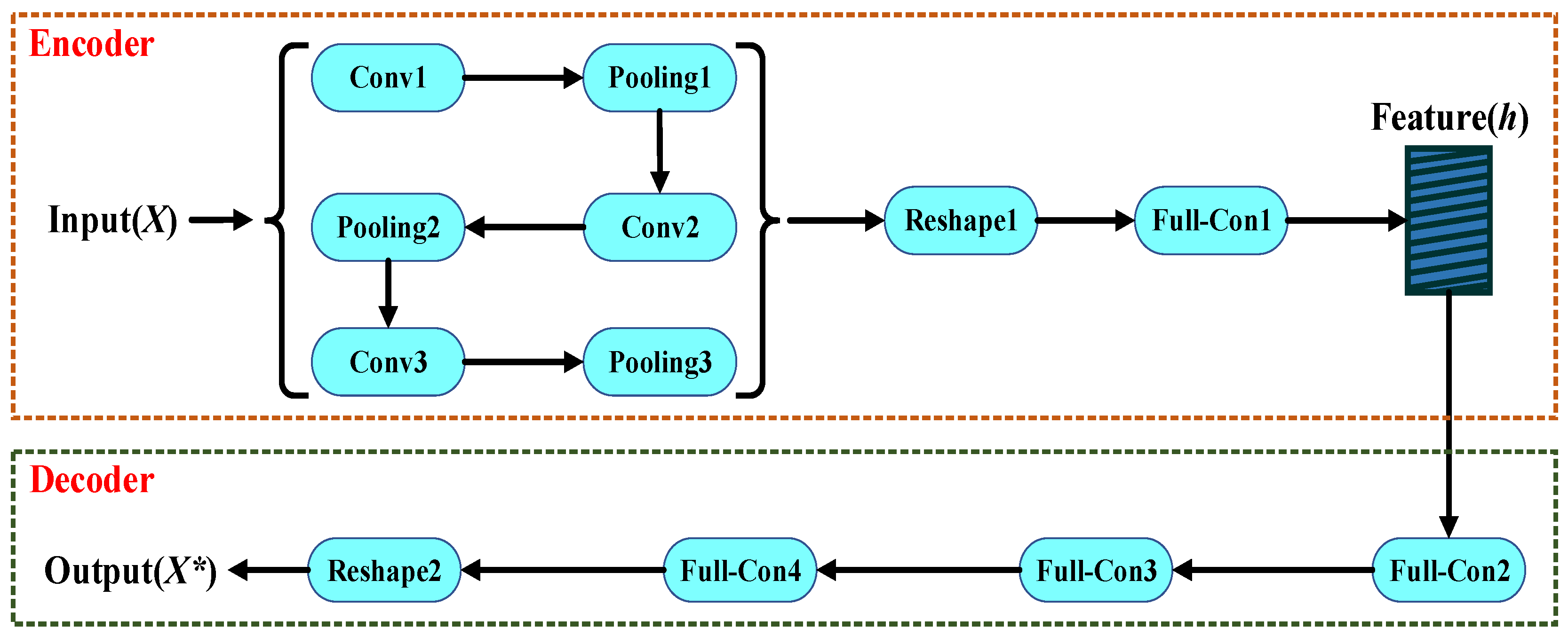
In this paper, the 1D-CAE network structure uses the one-dimensional convolutional neural network (1D-CNN) as an encoder for feature extraction. That is, the relationship between a microwave filter’s physical parameters and responses is established. After fully learning by the encoder, the physical parameters are predicted into the characteristic response by the decoder directly. As shown in Figure 1, the decoding part of 1D-CAE is applied to construct a novel surrogate model to displace the full-wave EM simulation, which greatly shortens the calculation time of MOEA/D. This paper uses the loss function to determine whether the 1D-CAE prediction is accurate. The MOEA/D algorithm based on the 1D-CAE network structure aims to:

(1) Multiple design objectives can be jointly optimized;

(2) Obtain comparable results as the traditional multi-objective design approach (directly using EM solver for MOEA/D);

(3) Finish the multi-objective design of the filter in a shorter time (a few hours to one day or so);

(4) When the specific characteristics of the filter are not considered, it can be universally used in most types of filters.

The remainder of this article is structured as follows. Section 2 discusses related works and methods, illustrates the basic theory of 1D-CAE network structure and the MOEA/D algorithm in terms of mathematical formulation, and introduces a detailed framework of 1D-CAE-based MOEA/D. In Section 3, the practicability and effectiveness of the presented technology are confirmed by two practical microwave filter design examples. Section 4 concludes the paper.

2. Materials and Methods

2.1. D-CAE Network Structure

2.1.1. Autoencoder’s Framework

Autoencoder is an artificial neural network that learns the efficient representation of input data. It is trained to try to reproduce input to output. The dimension of the encoder part is universally much smaller than that of the input data. So, AE can be applied for dimensionality reduction. By extracting features, AE also has the function of generating model, that is, it can randomly generate data similar to training data.

As shown in Figure 2, the typical structure of AE has two parts (encoder part and decoder part). The encoder part is composed of an input layer and a hidden layer, and it is used to extract latent features from original inputs. The original input data are $X=(x_1,\dots ,x_n)$, and the function of an encoder is to map the input sample into the latent space as the feature $h$:

$$h=Encoder(X),$$

(1)

The decoder part is composed of a hidden layer and an output layer. To obtain a decoded output vector $X*$, the decoder part maps the feature $h$ to the original input space:

$$X*=Decoder(h),$$

(2)

AE is committed to infinitely narrowing the gap between input samples and output samples. This gap is represented by the loss function:

$$L=K(X,X*),$$

(3)

2.1.2. One-Dimensional Convolutional Autoencoders

The traditional autoencoder can easily copy the input sample to the output sample. However, the scope of application of this model is limited. The model’s prediction ability will be greatly reduced when the input samples are too complex. For filter design, the relationship between the physical parameters of the filter and the S-parameters is complex. In this paper, the 1D-CAE network structure based on AE and 1D-CNN is adopted to build the surrogate model. Including three convolution layers, three pooling layers, a reshape module, and a full connection layer, namely conv1, pooling1, conv2, pooling2, conv3, pooling3, reshape1, and full-con1, the encoder module is used to encode the input data. The decoder module consists of the reshape operation and full connection layer, namely full-con2, full-con3, full-con4, and reshape2. Figure 3 is an internal detailed structure diagram of 1D-CAE. Different types of layers are described in detail below.

As a feature extractor, the convolution layer makes use of several convolution kernels for convolution calculation to obtain more features. Let $f_z$ indicate the output of the Z-th kernel. $f_z$ is determined as follows [33]:

$$f_z=ReLU\left(\sum X\odot {\omega }_z+b_z\right),$$

(4)

$$\mathrm{Re}\mathrm{LU}(x)=\max (0,x),$$

(5)

where $\odot$ represents convolution operation, ${\omega }_z$ is the Z-th convolution kernel, and $b_z$ is the offset corresponding to the Z-th convolution kernel. $Z$ indicates the number of channels. ReLU is a rectifier linear unit.

The pooling layer can reduce the parameters in the whole neural network. The common types of pooling layers are max pooling and average pooling. This paper adopts max pooling. Max pooling only retains the most significant features so that it can reduce the size of the training sample and improve computational efficiency. For the k-length feature of the convolution layer in the Z-th channel, the output of the pooling layer is determined by the following formula [33]:

$$P_z(n)=\underset{0\le n\le \frac{k}{st}}{\max }\left\{f_z(nS,(n+1)S)\right\},$$

(6)

where $f_z$ represents the input. $S$ is the size of the pooling window, and $st$ is the step size.

The reshape module transforms the extracted feature vector into a one-dimensional form to facilitate coding in the full connection layer. The calculation process is as follows [34]:

$$F=\sin \left(w_f\ast E+b_f\right),$$

(7)

where $E$ is the eigenvector output by the last level pooling layer, $w_f$ is the weight of the full connection layer, $b_f$ indicates the offset of a full connection layer, and sin represents a kind of activation function.

2.1.3. 1D-CAE Network Structure Introduction in Filter Design

For the encoding part of the 1D-CAE, the input is the real part and imaginary part of the filters S11 and S21, and the output is the geometric parameters of the filter to be optimized. On the contrary, the input of the decoding part is the geometric parameters to be optimized, and the real and imaginary parts of S11 and S21 are their outputs. Therefore, the whole 1D-CAE network structure is a system in which the input part is the real S11 and S21 and the output part is the predicted S11 and S21, that is, the generation model function of the 1D-CAE network structure.

For the actual optimization of this paper, the performance of the 1D-CAE network structure is reflected by the combination of rebuild loss ($L_r$) and forecast loss ($L_f$). Let us use rebuild loss to assess the performance of 1D-CAE network structure reconstruction filter features. Rebuild loss is determined by the following formula [27]:

$$L_r=\frac{1}{M}{\displaystyle \sum }_{i=1}^M\left|S_{em}-S_{pr}\right|,$$

(8)

where $M$ represents the total training data, $S_{em}$ represents the simulated S-parameters, and $S_{pr}$ is the S-parameters of the reconstructed 1D-CAE network structure.

The predicted losses are expressed as follows [27]:

$$L_f=\frac{1}{M}{\displaystyle \sum }_{i=1}^M\left|H_{em}-H_{pr}\right|,$$

(9)

where $M$ represents the total training data, $H_{em}$ represents the realistic value of the physical parameters, and $H_{pr}$ is the predicted physical parameters’ value.

The total loss function is determined by the following formula [27]:

$$L_t=L_r+k{L}_f,$$

(10)

where $k$ is a regularization parameter. So as to make the network prediction more accurate, it is essential to minimize the value of the loss function ($L_t$). In this paper, the Adam optimizer is used to optimize the loss function of the network.

2.2. MOEA/D Algorithm

2.2.1. Multi-Objective Optimization Problem

The multi-objective optimization problem (MOPs) makes multiple objectives as best as possible in a given region at the same time. It is expressed by the following formula:

$$\mathrm{Minimize}f(x)=\left(f_1(x),\dots ,f_M(x)\right)\mathrm{subject}\mathrm{to}x\in \mathrm{X},$$

(11)

where $x=(x_1,\dots ,x_{\mathrm{e}})$ represents the e-dimensional vector to be solved, $\mathrm{X}$ represents the boundary range of $x$, $f_i(x)$ represents the i-th objective function to be optimized, and $M$ is the dimension of the goal vector. MOPs cannot receive a single solution that can meet all objectives concurrently. Accordingly, the solution of MOPs is usually a set of equilibrium solutions. Suppose $x_{}^E$ and $x_{}^F$ are two solutions of the MOPs in (11); $x_{}^E$ is said to Pareto dominate $x_{}^F$ if and only if $f_i(x_{}^{{\rm E}})\le f_i(x_{}^{\mathrm{F}})$ for all $i\in \{1,2,\dots ,M\}$ and $f_j(x_{}^{{\rm E}})\le f_j(x_{}^{\mathrm{F}})$ for at least one $j\in \{1,2,\dots ,M\}$. A solution $x_{}^E$ is Pareto optimal when there is no $x_{}^{\mathrm{G}}\in \mathrm{X}$ that Pareto dominates $x_{}^E$. The Pareto optimal set consists of all Pareto optimal solutions, and the Pareto front (PF) is the projection of the Pareto optimal set in the objective space.

2.2.2. MOEA/D

MOEA/D disassembles the MOPs into several single-objective optimization subproblems with neighborhood relations, and each subproblem is a dissimilar set of all objectives. Then, by analyzing the information of adjacent problems, all subproblems are optimized concurrently by an evolutionary algorithm. Due to the decomposition operation, this method can well maintain the distribution of solutions. In addition, by analyzing the information of adjacent problems to optimize, it is effective to avoid falling into local optimum. The detailed introduction to the important part of the MOEA/D is as follows.

I.

Weight vector

In order to disassemble the MOPs into several single-objective subproblems, MOEA/D needs to distribute even weight vectors in the target space. The number of weight vectors is the same as the population size. If the population size is $N$, the number of weight vectors is $N$. Each weight vector turns the MOPs into a single-objective problem. $N$ sets of weight vectors are $N$ single-objective optimization problems and${\mathrm{w}}_N^{}=(w_{N1}^{},w_{N2}^{},\dots ,w_{NM}^{})$ is the N-th weight vector, so:

$$w_{N1}^{}+w_{N2}^{}+\dots +w_{NM}^{}=1,$$

(12)

where $M$ represents the number of problems to be optimized. In addition, the uniformity of weight vector distribution should be as good as possible to improve the accuracy of optimization results.

II.

Decomposition strategy

The MOEA/D aims to convert the multi-objective optimization problem to single-objective optimization problem through an aggregation function. The generally applied decomposition strategies include penalty-based boundary intersection (PBI), weighted sum (WS), and Tchebycheff (TCH), among which the WS cannot solve nonconvex functions. The Tchebycheff method is used in this paper. The formula of Tchebycheff method is expressed by the following formula:

$$\mathrm{Minimize}{g}^{\mathrm{TCH}}\left(xǀw,z^{\ast }\right)=\underset{i=1,2,\dots ,M}{\max }\left\{w_i\cdot \left|z_i^{\ast }-f_i(x)\right|\right\},$$

(13)

where $z$ is the optimization result to be achieved (the reference point). Take double objectives as an example, calculating $w_1\cdot \left|z_1^{\ast }-f_1(x)\right|$ and $w_2\cdot \left|z_2^{\ast }-f_2(x)\right|$, respectively, to take the maximum value. The larger the value, the farther away from the reference point on this objective function. Supposing $w_1\cdot \left|z_1^{\ast }-f_1(x)\right|$ is larger, please gradually change $x$ so that this value is closer and closer to $z^{\ast }$ until it reaches the corresponding point on Pareto front. This process is actually finding the minimum value of the function $g^{\mathrm{TCH}}(x)=w_1\cdot \left|z_1^{\ast }-f_1(x)\right|$. If $w_1\cdot \left|z_1^{\ast }-f_1(x)\right|$ reaches its minimum value, $w_2\cdot \left|z_2^{\ast }-f_2(x)\right|$will also reach its minimum value. This is true for weight vector $w$. Each weight vector obtains the corresponding solution in this way.

III.

Neighborhood structures

Neighborhood structure is determined by the Euclidean distance among the weight vectors, which is the key to generating a new solution. The MOEA/D assumes that the solutions on adjacent weight vectors are similar, and each weight vector has neighbors. After generating a new solution, compare the newly generated solution with all solutions in its neighborhood (including the current solution of the current subproblem). When the newly generated solution is better, all poor neighbors will be displaced by the newly generated solution.

2.3. Filter Design by Surrogate-Modeling-Assisted MOEA/D

In this paper, the samples generated by full-wave EM simulation are used to train a 1D-CAE network to obtain the microwave filter responses in a shorter time in the design space. MOEA/D is applied to calculate the geometric parameters of the filter that meet the design requirements. The complete process of microwave filter design by 1D-CAE-network-assisted MOEA/D is given in Figure 4. In this process, there are several key points that need to be described in detail:

(a) Step 2: Data collection step. The purpose of data acquisition is to collect a certain number of training and test sets to develop a surrogate model. A set of data sets consists of a set of geometric parameters of the filter and its corresponding S-parameters. Electromagnetic simulations were performed by a high frequency structure simulator (HFSS) to obtain training and test sets. The values of the geometric parameters (H) are determined by the following formulas:

$$H=H_0+k{H}_0,$$

(14)

where$H_0$is the initial geometric parameter of the filter (center point), $k$ is a random number in the data collection range, and this range is around the center point and is determined considering the characteristics of the filter in this example.

Next, we input $H_0$, $k$, the number of data acquisitions and the center frequency of the filter, and so on into the data acquisition system. The data acquisition system will automatically drive the HFSS to complete the acquisition process until the preset number of data acquisitions is reached and the system stops running. The entire process requires no human intervention.

(b) Step 3: Surrogate model construction step. In this step, the data set generated in step 2 is divided into test set and training set according to 1:5. The value of the loss function is calculated by Equation (10). The Adam optimizer is used to optimize the loss function of the network.

The complete steps of 1D-CAE-network-aided MOEA/D to design filter are as follows:

Input:

$〈1〉$ $H_0$,$k$, the number of data acquisitions;

$〈2〉$ A multi-objective filter design problem with m objectives;

$〈3〉$ Termination conditions (e.g., filter design goal, maximum number of iterations);

$〈4〉$ MOEA/D parameters: the number of sub-problems (N); the number of neighbors of each weight vector (T); the population size; uniformly distributed weight vector.

Output:

$〈1〉$ Filter geometry parameter values that meet design requirements.

Step 1: Determine a model step.

 Step 1.1: Establish a microwave filter model.

 Step 1.2: Determine the initial geometric parameters of the microwave filter, that is, $H_0$ in Equation (14).

Step 2: Data collection step.

 Step 2.1: The geometric parameter value H is obtained according to Equation (14), and then the response (S parameter) of this microwave filter is generated by HFSS simulation.

 Step 2.2: Save the S-parameters in the form of the real part and the imaginary part.

Step 3: Surrogate model construction step.

 Step 3.1: Training 1D-CAE network structure. The value of the loss function is calculated by Equation (10). The Adam optimizer is used to optimize the loss function of the network.

 Step 3.2: The surrogate model is constructed via the trained 1D-CAE network structure.

Step 4: MOEA/D step.

 Step 4.1: Based on the multiple design requirements of the microwave filter, the corresponding optimization subproblems are set up.

 Step 4.2: Initialize population.

  Step 4.2.1: Create an external population (EP) to store outstanding individuals, initially empty.

  Step 4.2.2: Calculate the Euclidean distance between any two weight vectors and find the T closest weight vectors to each weight vector. For $i=1,2,\dots ,N$, let $B(i)=\{i_1,\dots ,i_T\}$. $x_{{}_{}}^1,x_{}^2,\dots ,x_{}^N$are the nearest T weight vectors of $w_{j_{}}^{}$.

  Step 4.2.3: Generate an initial number of random $x_{{}_{}}^1,x_{}^2,\dots ,x_{}^N$, using the surrogate model to calculate the fitness function value.

  Step 4.2.4: Initialize $z=\{z_1,\dots ,z_M\}$.

 Step 4.3: Assign a weight vector to each subproblem.

 Step 4.4: Each subproblem crosses and mutates in the neighbor.

 Step 4.5: Update parent population according to the aggregation function value.

For $z_j=f_j(y_{}^{·})$,

  Step 4.5.1: Copy: randomly choose two indices l, q from B(i), and then generate a new solution $y$ from $x_{}^l$ and $x_{}^q$.

  Step 4.5.2: Repair: if an element of $y$ exceeds a preset bound, its value will be reset to the max or min of the bound (generates $y_{}^{·}$ from $y$).

  Step 4.5.3: Update$z$: For each$\mathrm{j}=1,2,\dots ,m$, judge whether $y$ can replace the original extreme value. If$z_j<f_j(y_{}^{·})$, set $F(y_{}^{·})$.

  Step 4.5.4: Update the domain solution B(i) for each weight vector $w_{j_{}}^{}$in the domain; if it is optimized, update it.

  Step 4.5.5: Update EP: Remove all vectors dominated by $F(y_{}^{·})$ from EP. Add $F(y_{}^{·})$ to EP if no vector dominates $F(y_{}^{·})$ in outer population (EP).

 Step 4.6: If the maximum number of iterations is reached, go to step 5. Otherwise, go to Step 4.2.

Step 5: Verification optimization result step.

 Step 5.1: The optimization results obtained in step 5 are simulated with HFSS.

 Step 5.2: If the results meet the design requirements, go to step 7. Otherwise, go to step 6.

Step 6: Update the geometric parameters online and then go to step 1.2 directly.

Step 7: Complete the design of a microwave filter.

3. Design Results

3.1. Sixth-Order Ceramic Filter

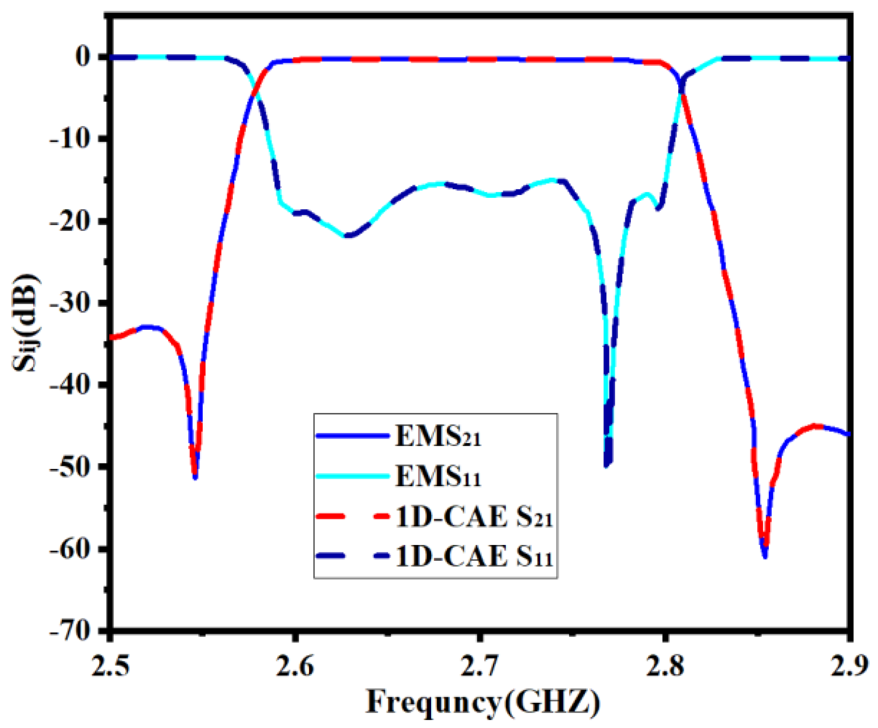
The first example shows the optimization design of a sixth-order ceramic bandpass filter. The structure of the sixth-order ceramic filter is shown in Figure 5. The finite transmission zeros of this microwave filter are$f_1$ = 2.552 GHz and$f_2$ = 2.858 GHz. The design geometric variables are H = [h1, h2, h3, h4, h5, h6]^T, and the design requirements of this filter are as follows:

• |S11| ≤ −20 dB, for 2.6 GHz ≤ ω ≤ 2.8 GHz;
• |S21| ≤ −50 dB, for ω = 2.552 GHz;
• |S21| ≤ −50 dB, for ω = 2.858 GHz.

The starting geometric parameter value of this example is H = [3.4, 3.3, 3.85, 3.9, 3.4, 3.4]^T (mm), and its EM response indicates that the response at the starting point is far away from the design requirements.

This example consists of two main steps. The first step is to develop a surrogate model based on 1D-CAE with the real part and imaginary part of the filter’s S11 and S21 as the model output and geometrical parameters as model inputs, i.e., H = [h1, h2, h3, h4, h5, h6]^T. The EM data are used to train the 1D-CAE. The second step is to apply the trained surrogate model to the multi-objective optimization design, and the geometric parameters can be adjusted repeatedly in the optimization process.

At first, the engineer needs to construct a 1D-CAE network structure. In Figure 6, the encoder part has a convolution layer, pooling layer (down-sampling), and full connection layer. A three-layer full connection constitutes the decoder part. The Conv1D (3, 32, 1) indicates a convolution layer. The first number (3) indicates that the convolution kernel is 3, the second number (32) indicates the number of output channels of this layer is 32 and the third number (1) indicates the stride is 1. Maxpool (3,3) represents a maximum pooling layer with a down-sampling factor value of 3 and stride size of 3. Full connection (N) represents a full connection layer with N nodes, where N is the dimension of the geometric parameters to be predicted by the filter. The input information includes real and imaginary parts of the S-parameters of 301 frequency points. After Conv1D (3, 32, 1), the input data are transformed into a matrix of 301 × 32 (32 channels, 301 indicates the length of a single channel). Next, the matrix became 101 × 32 after Maxpool (3,3).

Developing a 1D-CAE network structure requires a certain number of training sets and test sets. EM simulations are performed by a high-frequency structure simulator (HFSS) to obtain training sets and test sets. We set the range of the surrogate model to be k = [2% 2% 2% 2% 2% 2%]^T. This range is around the center point and is determined considering the characteristics of the filter in this example. Every time the geometric parameters change, the filter model is simulated based on this through the EM solver to gain the real part and imaginary part sample data of S11 and S21. So as to ensure the high accuracy of this model, 360 sets of data are obtained, including 288 training sample data and 72 test sample data. It should be noted that in the design process of the microwave filter, tuning is usually the most time consuming and may take several months. In contrast, the efficiency of this approach is sufficient even without parallel computing. If parallel computing is applied, the efficiency is quite high. In Figure 7, the comparison between EM responses and 1D-CAE network structure prediction is shown. It can be observed that the two results are completely consistent.

Table 1. Comparison of CPU time between HFSS and 1D-CAE.

	EM Simulation	1D-CAE Prediction
Completion time	3 min	0.017 s

shows a comparison of the two approaches (EM responses and 1D-CAE network structure prediction) in terms of CPU time. The EM responses time is viewed through the HFSS simulation process information interface after the simulation. 1D-CAE network structure prediction time is calculated by Equation (15). It can be observed that 1D-CAE not only achieves almost the same accuracy as HFSS simulation but also completes faster than EM simulation.

$$tim{e}_{1D-CAE}=\frac{time\_total}{n},$$

(15)

where $time\_total$ is the total predicted time of 1D-CAE. $n$ is the number of 1D-CAE predictions over this total time.

Once the surrogate model is trained well, it can be applied to the MOEA/D, in which the geometric parameters can be adjusted repeatedly. In MOEA/D, multiple design objectives of the filter are set as multiple subproblems. A low-complexity surrogate model based on 1D-CAE is constructed to form the results of the MOEA/D scalar subproblem, which tremendously improves the design efficiency. According to the design requirements of the filter, three objective functions are set for optimization:

$$Fi{t}_1=\max \left\{\left(f_l\le db\left(S_{11}\right)\le f_h\right)\right\}-(-20),$$

(16)

$$Fi{t}_2=\min \left\{\left(f_1-0.05\le db\left(S_{21}\right)\le f_1+0.05\right)\right\}-(-50),$$

(17)

$$Fi{t}_3=\min \left\{\left(f_2-0.05\le db\left(S_{21}\right)\le f_2+0.05\right)\right\}-(-50),$$

(18)

where $f_l$ is 2.6 GHz and $f_h$ is 2.8 GHz. $f_1$ = 2.552 GHz and $f_2$ = 2.858 GHz are the finite transmission zeros of this sixth-order ceramic bandpass filter.

About MOEA/D, the number of neighbors of each weight vector is set to 5, the population size is set to 350, and the maximum number of iterations is set to 60. In order to clearly show the optimization trend, every 10 iterations are defined as a stage, and the optimization results are extracted once. In the sixth stage, MOEA/D found the optimal solution of this sixth-order ceramic bandpass filter. Detailed general flow of this bandpass filter design is shown in Figure 8. The geometric parameters change in the whole process is shown in

Table 2. The geometric parameters’ change in the whole process.

Stage	h1	h2	h3	h4	h5	h6
0	3.400	3.300	3.850	3.900	3.400	3.400
1	3.374	3.365	3.845	3.883	3.370	3.407
2	3.350	3.370	3.845	3.853	3.370	3.385
3	3.335	3.370	3.845	3.845	3.370	3.360
4	3.330	3.370	3.845	3.845	3.370	3.357
5	3.330	3.369	3.845	3.845	3.370	3.348
6	3.329	3.369	3.845	3.845	3.373	3.330

. The EM responses at different stages are shown in Figure 9.

The comparisons of the proposed optimization and directly using the EM solver for MOEA/D are shown in

Table 3. Comparison of CPU time between two optimization design methods.

	Directly Using EM Simulation for MOEA/D	Proposed Optimization
Total EM simulation time	184.5 h	22.5 h
Time of surrogate model training	--	5 min
MOEA/D optimization time	185h	3.5min
Total time	185h	22.64h

. (The data values in Table 3 are missing because using the EM solver directly does not require training a surrogate model.) We can see that our proposed method can achieve an optimal EM solution in less time.

3.2. Seventh-Order Metal Cavity Bandpass Filter

In the second example, let us consider a seventh-order metal cavity bandpass filter with a center frequency of 1.791 GHz and a bandwidth of 30 MHz, as shown in Figure 10. The finite transmission zero of this seventh-order metal cavity bandpass filter is $f_1$ = 1.765 GHz. The design geometric variables are H = [w₁₂/w ₆₇, w₂₃/w₅₆, w₃₄/w_45, h₁/h₇, h₂/h₆, h₃/h₅, h₄]^T. The design requirements of the bandpass filter are as follows:

• | S11| ≤ −20dB, for 1.776 GHz ≤ ω ≤ 1.806 GHz;
• | S21| ≤ −90dB, for ω = 1.765 GHz;
• | S21| ≤ −40dB, for ω = 1.825 GHz.

The starting geometric parameter value of this example is H = [22.2, 17.23, 15.7, 6.63, 5.36, 5.6, 5.7]^T (mm), and its EM response indicates that the response at the starting point is far away from the design requirements.

The parameter values of each layer of 1D-CAE network structure are consistent with Figure 6. So as to guarantee the high accuracy of the 1D-CAE network structure, 550 sets of data, including 440 training sets and 110 test sets, are obtained by HFSS. In Figure 11, the comparison of EM responses with 1D-CAE network structure prediction is shown.

Table 4. Comparison of CPU time between HFSS and 1D-CAE.

	EM Simulation	1D-CAE Prediction
Completion time	12 min	0.02 s

shows a comparison for the two approaches (EM responses and 1D-CAE network structure prediction) in terms of the CPU time.

According to the design requirements of this filter, three objective functions are set for optimization:

$$Fi{t}_1=\max \left\{\left(f_l\le db\left(S_{11}\right)\le f_h\right)\right\}-(-20),$$

(19)

$$Fi{t}_2=\min \left\{\left(f_1-0.05\le db\left(S_{21}\right)\le f_1+0.05\right)\right\}-(-90),$$

(20)

$$Fi{t}_3=\min \left\{\left(f_2-0.05\le db\left(S_{21}\right)\le f_2+0.05\right)\right\}-(-40),$$

(21)

where $f_l$ is 1.776 GHz, $f_h$ is 1.806 GHz, $f_1$ = 1.765 GHz, and $f_2$ = 1.825 GHz.

MOEA/D parameters are the same as in the first example, but the maximum number of iterations is set to 50. In order to clearly show the optimization trend, every 10 iterations are defined as a stage, and the optimization results are extracted once. In the fifth stage, MOEA/D found the optimal solution. The geometric parameters’ change in the iterative process is shown in

Table 5. The geometric parameters’ change in the whole process.

Stage	w12/w67	w23/w56	w34/w45	h1/h7	h2/h6	h3/h5	h4
0	22.200	17.230	15.700	6.630	5.360	5.600	5.700
1	22.192	17.233	15.679	6.586	5.398	5.657	5.720
2	22.507	17.155	15.684	6.586	5.398	5.660	5.720
3	22.505	17.153	15.689	6.581	5.397	5.643	5.723
4	22.500	17.158	15.690	6.581	5.401	5.645	5.721
5	22.443	17.154	15.689	6.580	5.401	5.645	5.721

. The EM responses at different stages are shown in Figure 12.

The comparisons of the proposed optimization and directly using the EM solver for MOEA/D are shown in

Table 6. Comparison of CPU time between two optimization design methods.

	Directly Using EM Simulation for MOEA/D	Proposed Optimization
Total EM simulation time	615.5 h	110 h
Time of surrogate model training	--	7 min
MOEA/D optimization time	616 h	5 min
Total time	616 h	110.2 h

. (The data values in Table 6 are missing because using the EM solver directly does not require training a surrogate model.) We can see that our proposed method can achieve an optimal EM solution in less time.

4. Conclusions

A novel method merging MOEA/D and a 1D-CAE network structure is proposed to design microwave filters. In this new design method, the 1D-CAE network structure is introduced to replace the traditional full-wave simulation, which greatly reduces the design time of the filter. MOEA/D disassembles the MOPs into a set of single-objective optimization subproblems with neighborhood relations, and each subproblem is a dissimilar set of all objectives. Then, by analyzing the information of adjacent problems, all of the subproblems are optimized by an evolutionary algorithm concurrently. This new method is used to design two microwave filters in our examples. The design results show that the new method merging MOEA/D and the 1D-CAE network structure can be used to design filters that meet the requirements easily. With the help of the 1D-CAE network structure, the MOEA/D algorithm more easily avoids falling into the local optimum and completes the filter design in a shorter time than the EM-based microwave filter design.

In future work, we will continue our research from the following two aspects. First, we will try to apply the proposed technique to the design of other passive devices, such as antennas, couplers, duplexers, etc. Second, we will seek more reliable optimization methods to improve the generalization ability of surrogate models.

References

1. Cai, Y.X.; He, Y.J.; Zhou, H.W.; Liu, J.J. Design method of LCL filter for grid-connected inverter based on particle swarm optimi-zation and screening method. IEEE Trans. Power Electron. 2021, 36, 10097–10113. [Google Scholar] [CrossRef]
2. Zhang, D.H.; You, X.M.; Liu, S.; Yang, K. Multi-colony ant colony optimization based on generalized jaccard similarity rec-ommendation strategy. IEEE Access 2019, 7, 157303–157317. [Google Scholar] [CrossRef]
3. Chen, X.; Tian, Y.; Zhang, T.; Gao, J. Differential evolution based manifold gaussian process machine learning for microwave filter’s parameter extraction. IEEE Access 2020, 8, 146450–146462. [Google Scholar] [CrossRef]
4. Goudos, S.K.; Sahalos, J.N. Pareto optimal microwave filter design using multi-objective differential evolution. IEEE Trans. Antennas Propag. 2010, 58, 132–144. [Google Scholar] [CrossRef]
5. Yang, S.Y.; Ho, S.L.; Ni, G.Z.; Machado, J.M.; Wong, K.F. A new implementation of population based incremental learning method for optimizations in electromagnetics. IEEE Trans. Magn. 2007, 43, 1601–1604. [Google Scholar] [CrossRef]
6. Ho, S.L.; Yang, S. A population-based incremental learning method for robust optimal solutions. IEEE Trans. Magn. 2010, 46, 3189–3192. [Google Scholar] [CrossRef]
7. Yang, L.; Zhu, L.; Choi, W.-W.; Tam, K.-W.; Zhang, R.Q.; Wang, J.P. Wideband balanced-to-unbalanced bandpass filters syn-thetically designed with Chebyshev filtering response. IEEE Trans. Microw. Theory Technol. 2018, 66, 4528–4539. [Google Scholar] [CrossRef]
8. Li, X.; Zhang, X.; Lin, F. Multi-objective design of output LC filter for buck converter via the coevolving-AMOSA algorithm. IEEE Access 2020, 9, 11884–11894. [Google Scholar] [CrossRef]
9. Zobaa, A.F. Optimal multiobjective design of hybrid active power filters considering a distorted environment. IEEE Trans. Ind. Electron. 2013, 61, 107–114. [Google Scholar] [CrossRef] [Green Version]
10. Chen, B.-S.; Lee, M.-Y.; Chen, X.-H. Security-enhanced filter design for stochastic systems under malicious attack via smoothed signal model and multiobjective estimation method. IEEE Trans. Signal Process. 2020, 68, 4971–4986. [Google Scholar] [CrossRef]
11. Zhang, Q.; Li, H. MOEA/D: A multiobjective evolutionary algorithm based on decomposition. IEEE Trans. Evol. Comput. 2007, 11, 712–731. [Google Scholar] [CrossRef]
12. Fan, Z.; Li, W.; Cai, X.; Hu, K.; Lin, H.; Li, H. Angle-based constrained dominance principle in MOEA/D for constrained multi-objective optimization problems. IEEE Congr. Evol. Comput. 2016, 460–467. [Google Scholar] [CrossRef]
13. Qi, Y.; Ma, X.; Liu, F.; Jiao, L.; Sun, J.; Wu, J. MOEA/D with adaptive weight adjustment. Evol. Comput. 2014, 22, 231–264. [Google Scholar] [CrossRef] [Green Version]
14. Li, K.; Deb, K.; Zhang, Q.; Kwong, S. An evolutionary many-objective optimization algorithm based on dominance and decomposition. IEEE Trans. Evol. Comput. 2014, 19, 694–716. [Google Scholar] [CrossRef]
15. Li, K.; Zhang, Q.; Kwong, S.; Li, M.; Wang, R. Stable matching-based selection in evolutionary multi-objective optimization. IEEE Trans. Evol. Comput. 2014, 18, 909–923. [Google Scholar]
16. Feng, F.; Zhang, C.; Gongal-Reddy, V.-M.; Zhang, Q.-J.; Ma, J. Parallel space-mapping approach to EM optimization. IEEE Trans. Microw. Theory Technol. 2014, 62, 1135–1148. [Google Scholar] [CrossRef]
17. Feng, F.; Zhang, C.; Zhang, S.; Gongal-Reddy, V.-M.; Zhang, Q.-J. Parallel EM optimization approach to microwave filter design using feature assisted neuro-transfer functions. In Proceedings of the 2016 IEEE MTT-S International Microwave Symposium (IMS), San Francisco, CA, USA, 22–27 May 2016; pp. 1–3. [Google Scholar] [CrossRef]
18. Zhang, C.; Feng, F.; Gongal-Reddy, V.-M.; Zhang, Q.J.; Bandler, J.W. Cognition-driven formulation of space mapping for equal-ripple optimization of microwave filters. IEEE Trans. Microw. Theory Technol. 2015, 63, 2154–2165. [Google Scholar] [CrossRef]
19. Koziel, S.; Ogurtsov, S.; Bandler, J.W.; Cheng, Q. Reliable space-mapping optimization integrated with EM-based adjoint sensitivities. IEEE Trans. Microw. Theory Technol. 2013, 61, 3493–3502. [Google Scholar] [CrossRef]
20. Jin, J.; Feng, F.; Na, W.; Zhang, J.N.; Zhang, W.; Zhao, Z.H.; Zhang, Q.-J. Advanced cognition-driven EM optimization incor-porating transfer function-based feature surrogate for microwave filters. IEEE Trans. Microw. Theory Technol. 2021, 69, 15–28. [Google Scholar] [CrossRef]
21. Zhang, J.; Feng, F.; Na, W.; Jin, J.; Zhang, Q.J. Adaptively weighted training of space-mapping surrogates for accurate yield estimation of microwave components. In Proceedings of the 2020 IEEE/MTT-S International Microwave Symposium (IMS), Los Angeles, CA, USA, 18–27 June 2020; pp. 64–67. [Google Scholar] [CrossRef]
22. Zhang, W.; Feng, F.; Jin, J.; Zhang, Q.-J. Parallel multiphysics optimization for microwave devices exploiting neural network surrogate. IEEE Microw. Wirel. Components Lett. 2021, 31, 341–344. [Google Scholar] [CrossRef]
23. Zhang, C.; Na, W.; Zhang, Q.J.; Bandler, J.W. Fast yield estimation and optimization of microwave filters using a cogni-tion-driven formulation of space mapping. In Proceedings of the 2016 IEEE MTT-S International Microwave Symposium (IMS), San Francisco, CA, USA, 22–27 May 2016; pp. 1–4. [Google Scholar]
24. Zhang, J.; Feng, F.; Jin, J.; Zhang, Q.-J. Efficient yield estimation of microwave structures using mesh deformation-incorporated space mapping surrogates. IEEE Microw. Wirel. Components Lett. 2020, 30, 937–940. [Google Scholar] [CrossRef]
25. Feng, F.; Zhang, J.; Zhang, W.; Zhao, Z.; Jin, J.; Zhang, Q.-J. Coarse-and fine-mesh space mapping for EM optimization in-corporating mesh deformation. IEEE Microw. Wireless Compon. Lett. 2019, 29, 510–512. [Google Scholar] [CrossRef]
26. Sans, M.; Selga, J.; Rodríguez, A.; Bonache, J.; Boria, V.E.; Martín, F. Design of planar wideband bandpass filters from spec-ifications using a two-step aggressive space mapping (ASM) optimization algorithm. IEEE Trans. Microw. Theory Technol. 2014, 62, 3341–3350. [Google Scholar] [CrossRef]
27. Wang, Y.; Zhang, Z.; Yi, Y.; Zhang, Y. Accurate microwave filter design based on particle swarm optimization and one-dimensional convolution autoencoders. Int. J. RF Microw. Comput. Eng. 2021, 32, e23034. [Google Scholar] [CrossRef]
28. Zhang, Z.; Liu, B.; Yu, Y.; Cheng, Q.S. A microwave filter yield optimization method based on off-line surrogate model-assisted evolutionary algorithm. IEEE Trans. Microw. Theory Technol. 2022, 70, 1–10. [Google Scholar] [CrossRef]
29. Masci, J.; Meier, U.; Cireşan, D.; Schmidhuber, J. Stacked convolutional auto-encoders for hierarchical feature extraction. In Lecture Notes in Computer Science; Springer: Berlin/Heidelberg, Germany, 2011; pp. 52–59. [Google Scholar]
30. Geng, J.; Fan, J.C.; Wang, H.Y.; Ma, X.R.; Li, B.M.; Chen, F.L. High-resolution SAR image classification via deep convolu-tional autoencoders. IEEE Trans. Geosci. Remote Sens. 2015, 12, 2351–2355. [Google Scholar] [CrossRef]
31. Park, S.; Yu, S.; Kim, M.; Park, K.; Paik, J. Dual autoencoder network for retinex-based low-light image enhancement. IEEE Access 2018, 6, 22084–22093. [Google Scholar] [CrossRef]
32. Zhao, L.J.; Huang, H.K.; Li, X.; Ding, S.X.; Zhao, H.L.; Han, Z.Y. An accurate and robust approach of device-free local-ization with convolutional autoencoder. IEEE Internet Things J. 2019, 6, 5825–5840. [Google Scholar] [CrossRef]
33. Yu, J.; Zhou, X. One-dimensional residual convolutional autoencoder based feature learning for gearbox fault diagnosis. IEEE Trans. Ind. Informatics 2020, 16, 6347–6358. [Google Scholar] [CrossRef]
34. Wen, T.; Zhang, Z. Deep convolution neural network and autoencoders-based unsupervised feature learning of EEG signals. IEEE Access 2018, 6, 25399–25410. [Google Scholar] [CrossRef]
Figure 1. Surrogate model constructed by 1D-CAE.
Electronics 11 03309 g001
Figure 2. The typical structure of AE.
Electronics 11 03309 g002
Figure 3. The detailed structure of the 1D-CAE network structure.
Electronics 11 03309 g003
Figure 4. The complete flow diagram of the filter design technique.
Electronics 11 03309 g004
Figure 5. Structure of sixth-order ceramic filter.
Electronics 11 03309 g005
Figure 6. Detailed parameters of 1D−CAE network structure.
Electronics 11 03309 g006
Figure 7. Comparison between full−wave EM simulation result and 1D−CAE prediction result of the first example.
Electronics 11 03309 g007
Figure 8. General design flow of the filter.
Electronics 11 03309 g008
Figure 9. EM responses at different steps of the first example. (a) Return loss S11. (b) Insertion loss S21.
Electronics 11 03309 g009
Figure 10. Structure of seventh-order metal cavity bandpass filter.
Electronics 11 03309 g010
Figure 11. Comparison between full−wave EM simulation result and 1D−CAE prediction result of the second example.
Electronics 11 03309 g011
Figure 12. EM responses at different steps of the second example. (a) Return loss S11. (b) Insertion loss S21.
Electronics 11 03309 g012