Abstract
Knowledge distance is used to measure the difference between granular spaces, which is an uncertainty measure with strong distinguishing ability in a rough set. However, the current knowledge distance failed to take the relative difference between granular spaces into account under the given perspective of uncertain concepts. To solve this problem, this paper studies the relative knowledge distance of intuitionistic fuzzy concept (IFC). Firstly, a micro-knowledge distance (md) based on information entropy is proposed to measure the difference between intuitionistic fuzzy information granules. Then, based on md, a macro-knowledge distance (MD) with strong distinguishing ability is further constructed, and it is revealed the rule that MD is monotonic with the granularity being finer in multi-granularity spaces. Furthermore, the relative MD is further proposed to analyze the relative differences between different granular spaces from multiple perspectives. Finally, the effectiveness of relative MD is verified by relevant experiments. According to these experiments, the relative MD has successfully measured the differences in granular space from multiple perspectives. Compared with other attribute reduction algorithms, the number of subsets after reduction by our algorithm is in the middle, and the mean-square error value is appropriate.
1. Introduction
Granular computing (GrC) [1,2,3,4] is a new type of computing used to solve problems by simulating the cognitive mechanism of humans. Information granule is the fundamental element in GrC for constructing granular spaces. A granular space consists of several information granules and their relationships, while a granular structure consists of many granular spaces and their relationships. By fusing the structure and optimization approach of granularity, Pedrycz [2] introduced the notion of justifiable granularity. Yao [5,6] examined the two fields of three-way decision and GrC, as well as their interplay. Wang [7,8] reviewed the GrC work from three aspects, including granularity optimization, granularity switching, and multi-granulation computing.
As the main GrC model, rough set [9] is a useful tool for handling uncertain knowledge by utilizing existing information granules. Uncertainty measure is a crucial tool for data analysis in a rough set. Wang [10] introduced a series of uncertainty measures for selecting the optimal features effectively. Li [11] offered the axiom definition of uncertainty measure for covering information systems by using its information structures. Sun [12] investigated the fuzzy neighborhood multigranulation rough set model to construct uncertainty measures. In generalized rough set models, Wang [13] described new uncertainty measures from the perspectives of the upper and lower approximations. Nevertheless, these uncertainty measures struggle to distinguish the differences between granular spaces when they possess the same uncertainty. To address this issue, Qian [14,15] first introduced the concept of knowledge distance, and there have been several works on knowledge distance in recent years. Li [16] proposed an interval-valued intuitionistic fuzzy set to describe fuzzy granular structure distance, and proved that knowledge distance is a special form of intuitionistic fuzzy granular structure distance. Yang [17,18] proposed a partition-based knowledge distance based on the Earth Mover’s Distance and further established the fuzzy knowledge distance. Chen [19] presented a new measure formula of knowledge distance by using Jaccard distance to replace set similarity. To measure the uncertainty derived from the disparities between local upper and lower approximation sets, Xia [20] introduced the local knowledge distance.
In practical applications, the target concept may be vague or uncertain. As a classical soft computing tool, the intuitionistic fuzzy set [21] extends the membership from single value to interval value. For uncertain information, the intuitionistic fuzzy set has more powerful ability than the fuzzy set [22], and it is currently extensively applied in different fields, i.e., decision-making [23,24,25], pattern recognition [26,27], control and reasoning [28,29], and fuzzy reasoning [30,31]. In rough set, an intuitionistic fuzzy concept (IFC) can be characterized by a pair of lower and upper approximation fuzzy sets. There are many research works [32,33,34,35,36,37] on the combination between rough set and the intuitionistic fuzzy set. In particular, the uncertainty measure of IFC in granular spaces becomes a basic issue. A novel concept of an intuitionistic fuzzy rough set based on two universes was proposed by Zhang [32] along with a specification of the associated operators. On the basis of the rough set, Dubey [35] presented an intuitionistic fuzzy c-means clustering algorithm and applied it to the segmentation of the magnetic resonance brain images. Zheng [36] proposed an improved roughness method to measure the uncertainty of covering-based rough intuitionistic fuzzy sets. These works indicate that intuitionistic fuzzy set and rough set are suitable mathematical methods for studying vagueness and uncertainty. Current uncertainty measures failed to distinguish different rough granular spaces with the same uncertainty when they are used to describe an IFC; that is, it is difficult to reflect on the differences between them. However, in some situations, such as attribute reduction or granularity selection, the different rough granular spaces for describing an IFC are necessary to distinguish. To solve this problem, based on our previous works [17,18], two-layer knowledge distance measures—that is, micro-knowledge distance (md) and macro-knowledge distance (MD)—are constructed to reflect the difference between granular spaces for describing an IFC. Finally, in order to analyze the relative differences between rough granular spaces under certain prior granular spaces, the concept of relative MD applied to data analysis is also proposed.
The following are the main contributions of our paper: (1) Based on information entropy, md is designed to measure the difference among intuitionistic fuzzy information granules. (2) On the basis of md, MD with strong distinguishing ability is further constructed, which can calculate the difference between rough granular spaces for describing an IFC. (3) The relative MD is proposed to analyze the relative difference between two rough granular spaces from multiple perspectives. (4) An algorithm of attribute reduction based on MD or relative MD is presented, and its effectiveness is verified by relevant experiments.
The rest of this paper is arranged as follows. Section 2 introduces related preliminary concepts. In Section 3, the two types of information entropy-based distance measure (md and MD) are presented. Section 4 presents the concept of relative MD. The relevant experiments are reported in Section 5. Finally, in Section 6, conclusions are formed.
2. Preliminaries
This part will go through some of the core concepts. Let be an information system, where U, C, D and V represent the universe of discourse, condition attribute set, decision attribute set and attribute value set corresponding to each object, respectively, and is an information function that specifies the property value of each object x in U.
Definition 1
(Intuitionistic fuzzy set). Assume that U is the universe of discourse, the following is the definition of an intuitionistic fuzzy set I on U:
where and denote two nonempty finite sets on the interval [0, 1], which refer to the set of degrees of membership and non-membership of x on I, respectively, and satisfy the conditions: .
Note: For convenience, all I below are represented as intuitionistic fuzzy sets on U.
Definition 2
(Average step intuitionistic fuzzy set [38]). Assume that in , and , where , then,
where, . is therefore referred to as an average step intuitionistic fuzzy set on .
As well known, the information entropy as an uncertainty measure is proposed in rough set theory,
where, . Let U be a nonempty universe and I be an intuitionistic fuzzy set on U.
The information entropy of I can be expressed as follows:
- (1)
- When U is continuous.
- (2)
- When U is discrete.where, , and denotes the membership degree of belongs to the intuitionistic fuzzy set I.
To measure the information entropy of the rough granular space of the IFC, this paper further proposed the definition of average information entropy as follows:
- (1)
- When U is continuous, the average information entropy of the rough granular space of I can be denoted by:
- (2)
- When U is discrete, the average information entropy of the rough granular space of I can be denoted by:where, , and denotes the membership degree of x belongs to the intuitionistic fuzzy set I, is the average step intuitionistic fuzzy set of .
Definition 3
(Distance measure [39]). Assume that U is the universe of discourse; Y, P and Q are three finite sets on U. When meets the following criteria, it is considered a distance measure,
- (1)
- Positive: ;
- (2)
- Symmetric: ;
- (3)
- Triangle inequality: .
Definition 4
(Granularity measure [40]). Assume that in , G is a mapping from the power set of C to the real number set. For any , when G meets the following criteria, it is considered a granularity measure,
- (1)
- ;
- (2)
- ;
- (3)
- .
Definition 5
(Information measure [41]). Assume that in , H is a mapping from the power set of C to the real number set. For any , when H meets the following criteria, it is considered an information measure,
(1) ;
(2) ;
(3) .
3. Information-Entropy-Based Two-Layer Knowledge Distance Measure
Although there are many research works [42,43,44,45] on distance measures between intuitionistic fuzzy sets from different perspectives, when an IFC is characterized by different rough granular spaces, respectively, the present fuzzy set distance measures failed to capture the differences between these granular spaces. In addition, as explained in Section 1, when an IFC is defined by two granular spaces, the measure result (fuzziness or information entropy) may be the same. Nevertheless, this does not mean that these two granular spaces are absolutely equal, and the difference between them for characterizing an IFC cannot be reflected. To tackle the difficulties listed above, this paper proposed micro-knowledge distance and macro-knowledge distance based on information entropy, which construct the two-layer knowledge distance measure in this section.
Example 2.
Assume that in , , , and .
By Formula (2),
It shows that calculating the average information entropy does not necessarily distinguish and describe two different rough granular spaces. Although the average information entropy values of and are the same, is superior to in terms of granularity selection, since has a coarser granularity and has a stronger generalization ability for describing IFC.
Assume , A is a finite set on U. Then, we call the intuitionistic fuzzy set generated by A as the intuitionistic fuzzy information granule (), abbreviated as .
Example 3
(Continued example 1). Let and , then:
Definition 6
(Micro-knowledge distance). Assume in , and are two intuitionistic fuzzy information granules on U, hence, the following is the definition of the md formula:
Theorem 1.
is a distance measure.
Proof of Theorem 1.
Let , and be three intuitionistic fuzzy information granules. Let:
Because , then .
Then .
According to Definition 3, conditions (1) and (2) are obviously satisfied, Therefore, is a distance measure. □
Example 4.
Assume that in , , is an intuitionistic fuzzy set on U, and are two finite sets on U.
Then,
From Definition 6,
Theorem 2.
Let Y, P and Q be three intuitionistic fuzzy sets on U. If , then .
Proof of Theorem 2.
According to condition, because , obviously,
Then,
Therefore, holds. Similarly, it is easy to get . □
Theorem 3.
Let Y, P and Q be three intuitionistic fuzzy sets on U. If , then .
Proof of Theorem 3.
Theorem 3 obviously holds.
Then
Therefore, . □
Based on md, this research further created MD, which is formulated as follows, to express the difference between two rough granular spaces for characterizing an IFC.
Definition 7
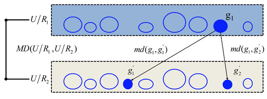
(Macro-knowledge distance). Assume that in , , and are two granular spaces induced by and , respectively. Then, the following is the definition of MD between and .
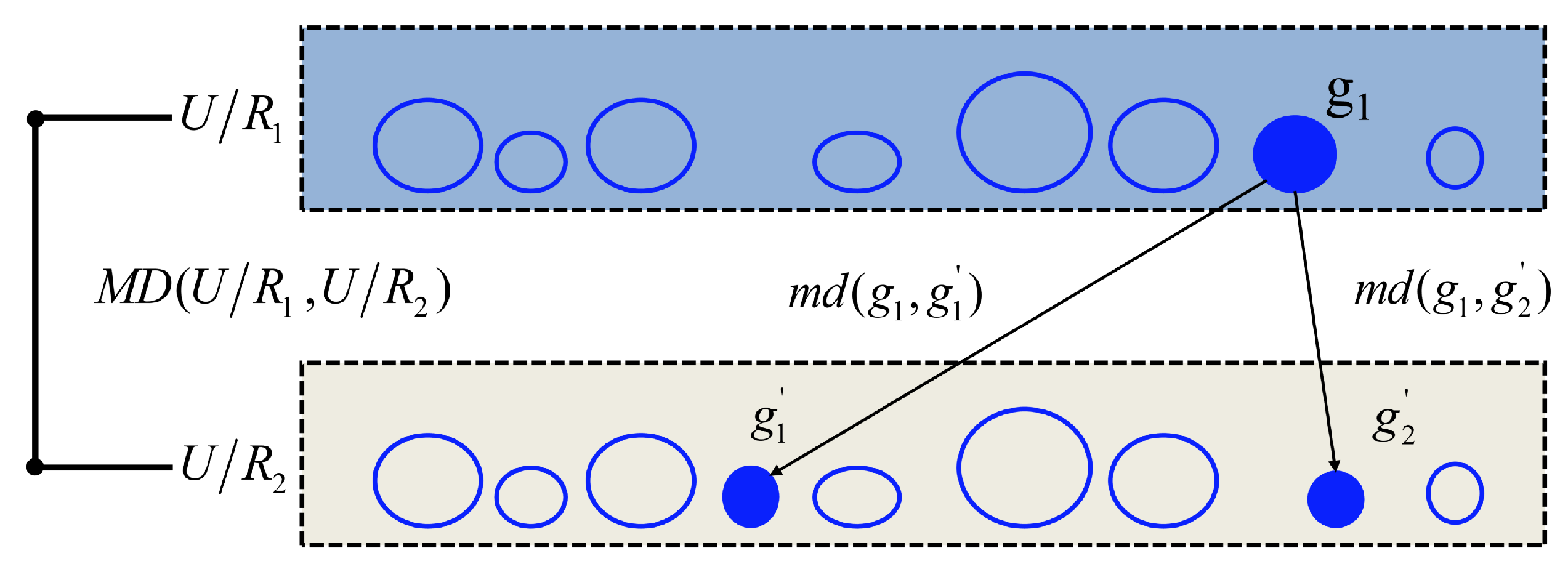
where, and . Figure 1 shows the relationship between md and MD.

Figure 1.
The relationship between md and MD.
Suppose that is a granular space on U induced by , where , Then, .
For example,
Theorem 4.
is a distance measure.
Proof of Theorem 4.
Assume that in , , and are three granular spaces induced by , and , respectively. Obviously, is positive and symmetric.
From Theorem 1,
Then,
Therefore, from Definition 3, is a distance measure. □
In fact, md measures the difference between two sets, and MD measures the difference between two rough granular spaces, which integrates the md of all sets of the two granular spaces. According to Theorem 1, Theorem 4 and Formula (4), as long as md in MD is a distance measure, then MD is a distance measure.
Example 5
(Continued Example 2). According to Formula (3),
Theorem 5.
Assume that in , . If , then .
Proof of Theorem 5.
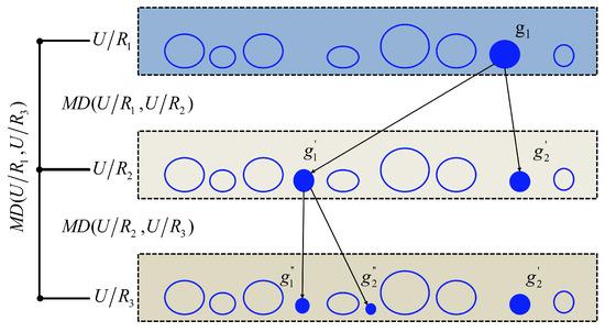
As shown in Figure 2, suppose , and are three granular spaces induced by , and , respectively. Because , so . For simplicity, supposing only one granule can be subdivided into two finer sub-granules and by and only one granule can be subdivided into two finer sub-granules and by (Because more sophisticated examples may be turned into this scenario, this essay will not go through them again).

Figure 2.
The relationship of MD among three granular spaces.
According to the above assumption, , , , ⋯, , , , , ⋯, , namely, and . Then, from Definition 7,
Because ,
According to Theorem 2, because and , then
Therefore, holds. Similarly, it is easy to get . □
In this paper, the finest and coarsest granular spaces are represented by and , respectively. The following corollaries derive from Theorem 5:
Corollary 1.
Assume that in , . If , then .
Corollary 2.
Assume that in , . If , then .
Theorem 6.
Assume that in , . According to Definition 4, is a granularity measure.
Proof of Theorem 6.
Suppose that ,
(1) From Theorem 4, ;
(2) When , obviously, ;
(3) From Corollary 1, if , then . □
Theorem 7.
Assume that in , . According to Definition 5, is an information measure.
Proof of Theorem 7.
Suppose that ,
(1) From Theorem 4, ;
(2) When , obviously, ;
(3) From Corollary 2, if , then . □
Theorem 8.
Assume that in , , then .
Proof of Theorem 8.
For simplicity, based on the proof of Theorem 5,
Similarly,
Because , and .
According to Theorem 3,
□
According to Theorem 8, from the perspective of distance, the granular spaces in hierarchical granular structure are linearly additive, which can be explained by Figure 2 intuitively. Moreover, the following corollaries hold:
Corollary 3.
Assume that in , . If , then
.
Corollary 4.
Assume that in , . If , then,
.
Corollary 5.
Assume that in , . Then .
Proof of Corollary 5.
Therefore, holds. □
From Corollary 3 and Theorem 6, for an IFC, the larger the granularity difference between granular spaces in hierarchical granular structure, the larger MD between them. From Corollary 4 and Theorem 7, for an IFC, the larger the information difference between granular spaces in hierarchical granular structure, the larger MD between them. From Corollary 5, the larger the information measure, the smaller the granularity measure, and one measure value can be deduced from another.
Note: By using a suitable md in Formula (3), the method of this paper is able to extend to quantify the difference between any types of granular spaces. These specifics are outside the scope of this paper’s discussion.
4. Relative Macro-Knowledge Distance
Section 3 has constructed an MD based on md, which described the difference between two rough granular spaces of IFC. We regarded this knowledge distance as absolute. Because in data analysis, sometimes some conditions are known, it is necessary to analyze the differences between rough granular spaces at this time; that is, to analyze the differences between rough granular spaces under different prior granular spaces. Inspired by Wang [46], this section proposes the concept of relative MD and analyzes its properties.
Definition 8
(Relative macro-knowledge distance). Assume that in , , is the prior granular space on U, and are two granular spaces induced by and , respectively. Then, the relative MD of and under is defined as:
where, and .
Based on the original MD, this definition adds prior granular space , which reflects the relative differences between two rough granular spaces from different perspectives.
Theorem 9.
is a distance measure.
Proof of Theorem 9.
Assume that in , is the prior granular space on U. , and are three granular spaces induced by , and , respectively. Obviously, is positive and symmetric.
According to Theorem 1,
Then,
Therefore, from Definition 3, is a distance measure. □
Example 6.
Assume that in , , . and . Under the prior granular spaces and
, the relative MD of and are as follows:
From Examples 5 and 6, after adding the prior granular space, the difference between the two rough granular spaces may change, and when the prior granular space is different, the obtained results may also be different.
Theorem 10.
Assume that in , is the prior granular space on U. If , then .
Proof of Theorem 10.
According to the conditions, , then .
So, .
According to Theorem 2,
Therefore, holds.
Similarly, it is easy to get
. □
Theorem 11.
Assume that in , is the prior granular space on U. If , then .
Proof of Theorem 11.
According to Theorem 10, it can be deduced from condition . Additionally, according to Theorem 3,
. Then,
Therefore,
holds. □
From Theorem 11, under the same prior granular space, the relative MD is linearly additive.
Theorem 12.
Assume that in , and are two prior granular spaces on U, respectively, . If ,
then .
Proof of Theorem 12.
Similarly,
According to , . Obviously,
Therefore, holds. □
Corollary 6.
Assume that in , , σ is the prior granular space on U, then .
Proof of Corollary 6.
□
Corollary 7.
Assume that in , , ω is the prior granular space on U, then .
Proof of Corollary 7.
□
Note: From Example 6, when the prior granular space is not the most refined, the relative MD may also be zero. Therefore, the prior granular space is the most refined granular space, which is only a sufficient condition for the relative MD to be zero, not a necessary condition.
According to Corollary 6, the absolute MD is the relative MD without any prior granular space; that is, the absolute MD can be viewed as a special case of the relative MD. By Corollary 7, when the prior granular space is fine enough, the relative MD between two different rough granular spaces has been infinitely reduced or even to zero. Combining Theorem 12, it follows that is true when .
That is, .
Theorem 13.
Assume that in , . Then
.
Proof of Theorem 13.
According to Theorem 3,
Therefore,
holds. □
From Theorem 13, an absolute MD was divided into the sum of two unidirectional relative MD in different directions. That is, the absolute MD of the two granular spaces is equal to the relative MD of the two granular spaces when the prior granular space is one of the two granular spaces, plus the relative MD of the two granular spaces when the prior granular space is the other granular space of the two granular spaces. This theoretically explains the dialectical unity of relative MD and absolute MD.
5. Experiment and Analysis
This section verifies that MD has a good advantage when describing IFC in multi-granularity space through relevant experiments. The experimental environments are Windows 10, Intel Core (TM) I5-10500 CPU (3.10 GHz) and 16GB RAM. The experimental platform is MATLAB 2022a. We filtered out nine datasets with decision attributes and a sufficient number of conditional attributes from UCI [47] and Dryad. Meanwhile, we removed attributes from some datasets that are completely independent of the decision attributes, such as serial number and date. The dataset’s basic information is recorded in Table 1, and experiments will use the following formula [48] to convert numerical values to discrete values. For convenience, the ID numbers in Table 1 will be used to represent the datasets.
where represent the attribute value, represent the minimum value of and represent the standard deviation of the attribute.

Table 1.
Experimental dataset.
5.1. Monotonicity Experiment
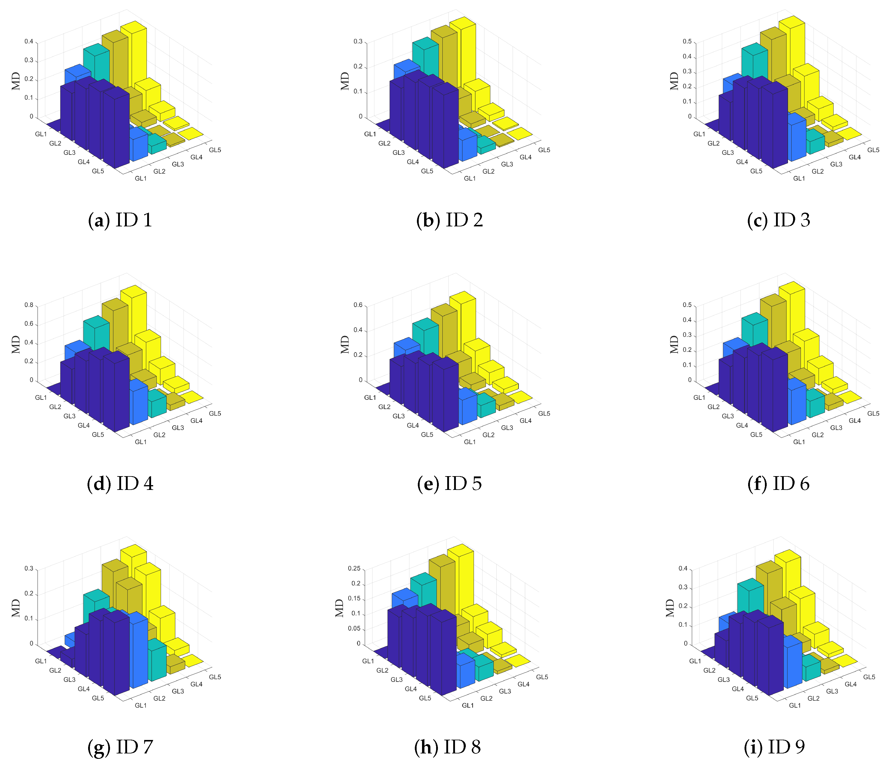
In this experiment, some attributes of the dataset in Table 1 were selected. Suppose is a hierarchical quotient space structure consisting of five granularity layers. , represent attribute sets, and . As shown in Figure 3, this figure shows that the behavior of each dataset is similar; that is, MD increases with the increase in the granularity difference between two granular spaces, and conversely, MD decreases with the decrease in the granularity difference between two granular spaces. Table 2 summarizes the changes in the two measures (granularity measure and information measure) based on MD in a hierarchical quotient space structure as the granularity layer becomes finer. The findings indicate that these two measures can provide additional information for assessing the uncertainty of fuzzy concepts. These findings support Theorems 6 and 7. The granularity measure decreases as the available information increases, while the information measure increases as the available information increases. According to Table 2, Corollary 5 can also be verified, the sum of granularity measure and information measure is fixed, and the result is .
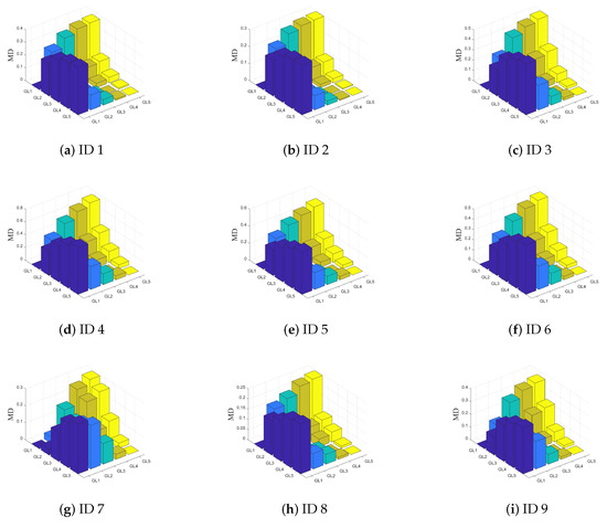
Figure 3.
The change of MD between different granular spaces. Each dataset is represented by ID number.

Table 2.
Granularity measure and Information measure.
5.2. Attribute Reduction
The so-called attribute reduction is to delete the irrelevant or unimportant attributes under the condition that the classification ability of the knowledge base remains unchanged. In data analysis, deleting unnecessary attributes can greatly improve the efficiency of data analysis, and the subset derived from attribute reduction with prior granular space may be different from the subset derived from attribute reduction without prior granular space. Aiming at this problem, this section makes a comparative experiment of attribute reduction based on relative MD in different prior granular spaces and attribute reduction based on absolute MD; in this paper, the attributes that divide the prior granular space are called prior conditions.
Some attributes of the dataset in Table 1 were selected in the experiment. Taking the calculation of attribute reduction based on relative MD as an example, Algorithm 1 is the algorithm used in the experiment. Attribute reduction based on absolute MD only needs to change the fourth step in Algorithm 1 to delete the first and last items in ; that is, without any prior conditions. In this paper, Algorithm 2 is used to represent attribute reduction based on absolute MD. Suppose an information system , then the calculation formula of attribute importance is as follows:
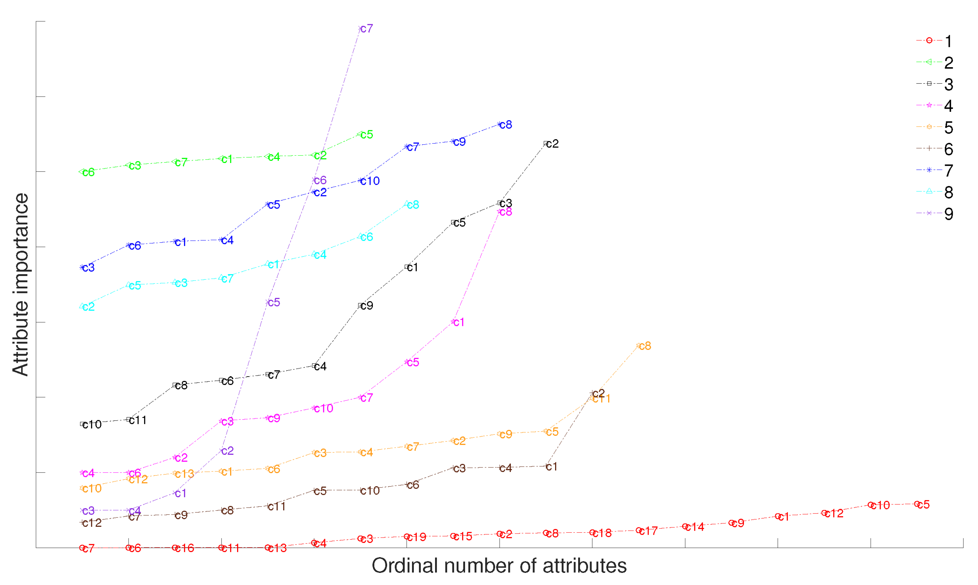
As shown in Figure 4, the attribute importance represents MD between the granular space after removing attribute i in the dataset and the granular space without removing this attribute. The larger the distance, the higher the attribute importance degree, and represents attribute i. Therefore, in this paper, the attributes with the largest and smallest attribute importance of the dataset are selected as prior conditions, and attribute reduction based on relative MD is carried out. Moreover, attribute reduction based on absolute MD is also performed without any prior conditions.
| Algorithm 1 Attribute reduction based on relative MD |
|
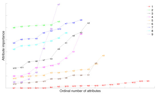
Figure 4.
Attribute importance of different attributes.
(Note: Figure 4 is only used to analyze the importance of the conditional attribute of a single system, so there is no correlation between the height of the line graph of different systems).
As shown in Table 3, in the attribute reduction based on absolute MD, is the maximum absolute MD between the granular space divided by attribute subsets after attribute reduction and the granular space divided by all attributes. In attribute reduction based on relative MD, is the maximum relative MD between the granular space divided by attribute subsets after attribute reduction and the granular space divided by all attributes. This paper sets to 0.003 and 0.006 for comparison. In the table, numbers are directly used to represent the serial numbers of the conditional attributes.

Table 3.
Attribute reduction on each dataset based on different situations.
(1) When the prior conditions are more important attributes, the number of attributes is significantly reduced compared to the attribute reduction based on absolute MD, which shows that selecting more important properties increases the cognitive ability of the system, consistent with Theorem 12.
(2) When the prior condition is an unimportant attribute, compared with the prior condition is an important attribute, the number of subsets after attribute reduction is usually more, which also indicates that the more important the prior condition is, the more cognitive ability of the attribute to the system can be improved.
(3) When is different—that is, the maximum MD between the granular space remains conditionally divided after attribute reduction and the granular space divided without reduction changes—the subsets after attribute reduction may be different, which illustrates the efficiency of this algorithm. The algorithm will obtain different attribute subsets as the requirements increase and decrease.
(4) The reduced attributes are all attributes with low attribute importance, which shows the effectiveness of this algorithm in calculating attribute importance.
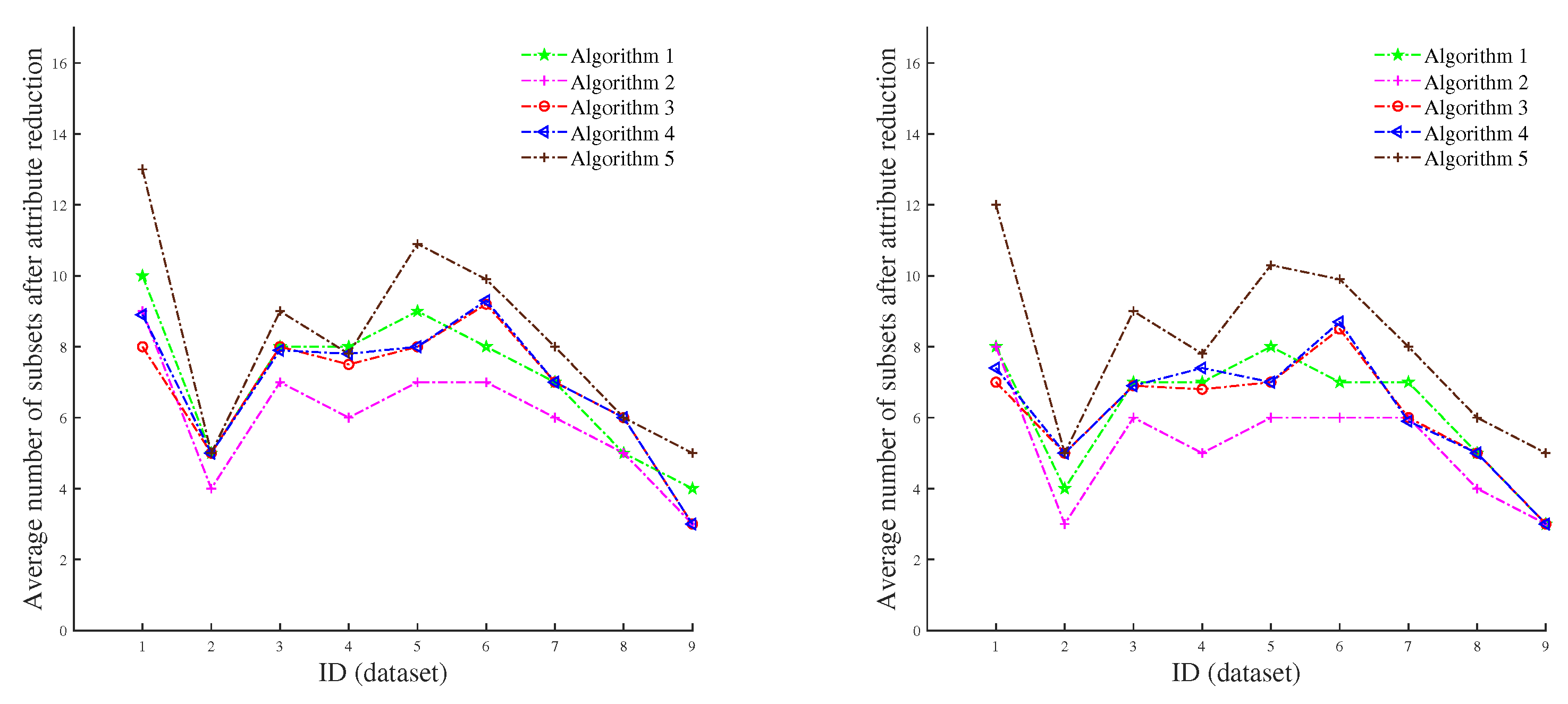
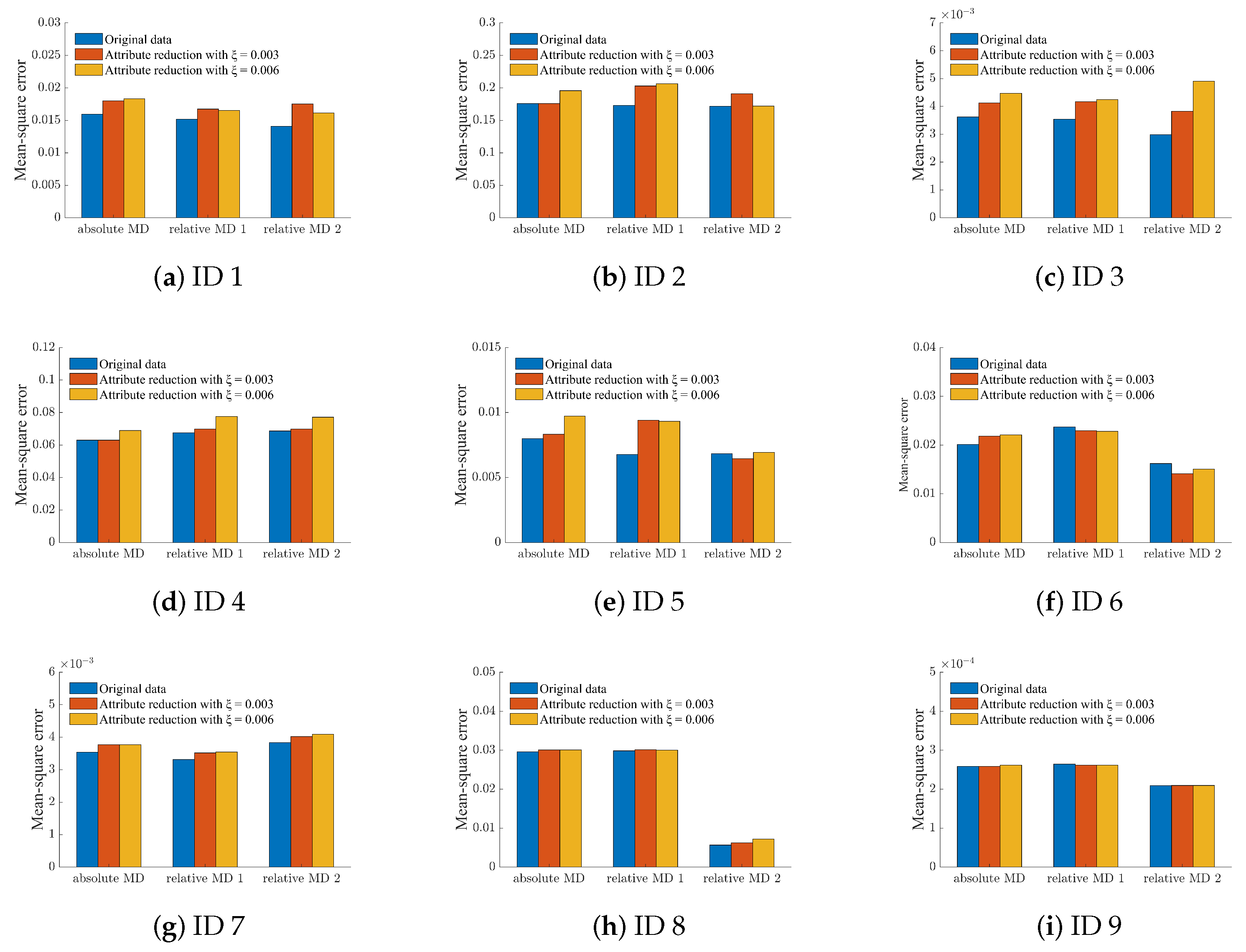
As shown in Figure 5, Algorithm 1 and Algorithm 2, respectively, represent the attribute reduction based on absolute MD and the attribute reduction based on relative MD with important condition as a prior condition proposed in this paper. Algorithm 3, Algorithm 4, and Algorithm 5 denote three attribute reduction algorithms based on Mi’s fuzziness, entropy-based fuzziness, and secondary fuzziness, respectively, where the left figure shows the case of = 0.003, and the right figure shows the case of = 0.006. From Figure 5, the number of remaining attribute subsets in Algorithm 1 after attribute reduction is appropriate. In addition, after adding the prior conditions, the number of subsets obtained after attribute reduction is significantly reduced in Algorithm 2, indicating that our algorithm greatly improves the cognitive ability of the system. Figure 6 shows the average value of the mean-square error before and after attribute reduction in three different regression models (random forest regression, decision tree regression and GBDT regularization) after the normalization of the nine datasets. In the figure, the prior condition of relative MD1 is the least important attribute, and the prior condition of relative MD2 is the most important attribute. After attribute reduction, we discover that the mean-squared error does not significantly change, and sometimes even decreases. This shows the feasibility of our algorithm and also shows that the algorithm can be effectively used in data analysis.
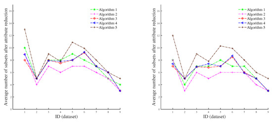
Figure 5.
Average number of attribute subsets after five different attribute reductions.

Figure 6.
Average value of the mean-square error on each dataset. Each dataset is represented by ID number.
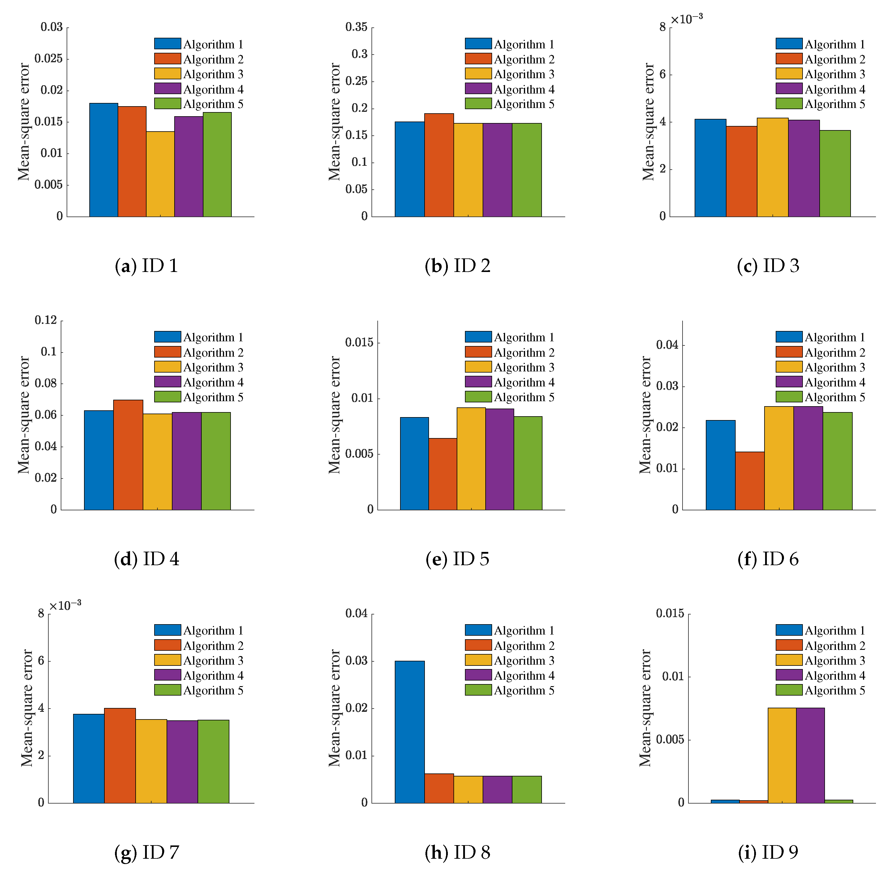
This paper also conducted a series of comparative experiments using the five algorithms mentioned above to compare the mean-square error values following the reduction of five different attributes. The experimental results are shown in Figure 7. In order to unify the standard, = 0.003 is used. Except for the datasets with ID 8 and ID 9, the mean-square error values obtained by our algorithm are in the middle. From Figure 6, after attribute reduction of dataset ID 8 and dataset ID 9, the mean-square error does not change much. Therefore, the reason for this result is that the correlation between some attributes of the dataset itself and the decision attributes is too large or too small. There is still room for improvement in this regard.
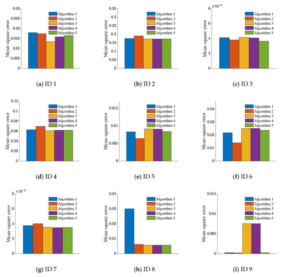
Figure 7.
Average value of the mean-square error of five different attribute reductions. Each dataset is represented by ID number.
6. Conclusions and Discussion
In this paper, the macro-knowledge distance of intuitionistic fuzzy sets is proposed to measure the difference between granular spaces effectively. Under the given perspective of uncertain concepts, the current knowledge distance failed to account for the relative difference between granular spaces. As a result, we further propose the relative macro-knowledge distance and demonstrate its practicability through relative attribute reduction experiments. These results provide a new perspective to current knowledge distance research by measuring the relative differences between different granular spaces under prior granular spaces. The conclusions are as follows:
(1) Macro-knowledge distance increases with the increase in the granularity difference between two granular spaces, and vice versa. The sum of granularity measure and information measure is always .
(2) After attribute reduction, the number of subsets obtained by our algorithm is appropriate, and in comparison to other algorithms, our mean square error is suitable. In the analysis of data, the more important the prior condition is, the more it can improve the cognitive ability of the attributes.
Under specific circumstances, the relative macro-knowledge distance is able to remove unnecessary attributes in practical applications, which can significantly increase the accuracy of attribute reduction and the effectiveness of data analysis. The characteristics of the data will be more thoroughly understood during the attribute reduction process.
Author Contributions
Conceptualization, J.Y. and X.Z.; methodology, J.Y., X.Q. and X.Z.; writing—original draft, J.Y. and X.Q; writing—review and editing, J.Y., X.Q., G.W. and B.W.; data curation, G.W., X.Z. and B.W.; supervision, X.Z. All authors have read and agreed to the published version of the manuscript.
Funding
This work is supported by the National Science Foundation of China (No. 62066049), Excellent Young Scientific and Technological Talents Foundation of Guizhou Province (QKH-platform talent[2021] No. 5627), National Science Foundation of Chongqing (cstc2021ycjh-bgzxm0013), Guizhou Provincial Science and Technology Project (QKH-ZK [2021]General 332), Science Foundation of Guizhou Provincial Education Department (QJJ2022[088]), The Applied Basic Research Program of Shanxi Province (No. 201901D211462), Electronic Manufacturing Industry-University-Research Base of Ordinary Colleges and Universities in Guizhou Province (QJH-KY-Zi [2014] No. 230-2).
Institutional Review Board Statement
Not applicable.
Informed Consent Statement
Not applicable.
Data Availability Statement
Not applicable.
Acknowledgments
This study was completed at the Chongqing Key Laboratory of Computational Intelligence, Chongqing University of Posts and Telecommunications, and the authors would like to thank the laboratory for its assistance.
Conflicts of Interest
The authors declare no conflict of interest.
References
- Yao, Y.Y. The art of granular computing. In Proceedings of the International Conference on Rough Sets and Intelligent Systems Paradigms, Warsaw, Poland, 28–30 June 2007; pp. 101–112. [Google Scholar]
- Bargiela, A.; Pedrycz, W. Toward a theory of granular computing for human-centered information processing. IEEE Trans. Fuzzy Syst. 2008, 16, 320–330. [Google Scholar] [CrossRef]
- Yao, J.T.; Vasilakos, A.V.; Pedrycz, W. Granular computing: Perspectives and challenges. IEEE Trans. Cybern. 2013, 43, 1977–1989. [Google Scholar] [CrossRef] [PubMed]
- Yao, Y.Y. Granular computing: Basic issues and possible solutions. In Proceedings of the 5th Joint Conference on Information Sciences, Atlantic City, NJ, USA, 27 February–3 March 2000; Volume 1, pp. 186–189. [Google Scholar]
- Yao, Y.Y. Set-theoretic models of three-way decision. Granul. Comput. 2021, 6, 133–148. [Google Scholar] [CrossRef]
- Yao, Y.Y. Tri-level thinking: Models of three-way decision. Int. J. Mach. Learn. Cybern. 2020, 11, 947–959. [Google Scholar] [CrossRef]
- Wang, G.Y.; Yang, J.; Xu, J. Granular computing: From granularity optimization to multi-granularity joint problem solving. Granul. Comput. 2017, 2, 105–120. [Google Scholar] [CrossRef]
- Wang, G.Y. DGCC: Data-driven granular cognitive computing. Granul. Comput. 2017, 2, 343–355. [Google Scholar] [CrossRef]
- Pawlak, Z. Rough sets. Int. J. Comput. Inf. Sci. 1982, 11, 341–356. [Google Scholar] [CrossRef]
- Wang, C.Z.; Huang, Y.; Shao, M.W.; Hu, Q.H.; Chen, D.G. Feature selection based on neighborhood self-information. IEEE Trans. Cybern. 2019, 50, 4031–4042. [Google Scholar] [CrossRef]
- Li, Z.W.; Zhang, P.F.; Ge, X.; Xie, N.X.; Zhang, G.Q. Uncertainty measurement for a covering information system. Soft Comput. 2019, 23, 5307–5325. [Google Scholar] [CrossRef]
- Sun, L.; Wang, L.Y.; Ding, W.P.; Qian, Y.H.; Xu, J.C. Feature selection using fuzzy neighborhood entropy-based uncertainty measures for fuzzy neighborhood multigranulation rough sets. IEEE Trans. Fuzzy Syst. 2020, 29, 19–33. [Google Scholar] [CrossRef]
- Wang, Z.H.; Yue, H.F.; Deng, J.P. An uncertainty measure based on lower and upper approximations for generalized rough set models. Fundam. Informaticae 2019, 166, 273–296. [Google Scholar] [CrossRef]
- Qian, Y.H.; Liang, J.Y.; Dang, C.Y. Knowledge structure, knowledge granulation and knowledge distance in a knowledge base. Int. J. Approx. Reason. 2009, 50, 174–188. [Google Scholar] [CrossRef]
- Qian, Y.H.; Li, Y.B.; Liang, J.Y.; Lin, G.P.; Dang, C.Y. Fuzzy granular structure distance. IEEE Trans. Fuzzy Syst. 2015, 23, 2245–2259. [Google Scholar] [CrossRef]
- Li, S.; Yang, J.; Wang, G.Y.; Xu, T.H. Multi-granularity distance measure for interval-valued intuitionistic fuzzy concepts. Inf. Sci. 2021, 570, 599–622. [Google Scholar] [CrossRef]
- Yang, J.; Wang, G.Y.; Zhang, Q.H.; Wang, H.M. Knowledge distance measure for the multigranularity rough approximations of a fuzzy concept. IEEE Trans. Fuzzy Syst. 2020, 28, 706–717. [Google Scholar] [CrossRef]
- Yang, J.; Wang, G.Y.; Zhang, Q.H. Knowledge distance measure in multigranulation spaces of fuzzy equivalence relations. Inf. Sci. 2018, 448, 18–35. [Google Scholar] [CrossRef]
- Chen, Y.M.; Qin, N.; Li, W.; Xu, F.F. Granule structures, distances and measures in neighborhood systems. Knowl.-Based Syst. 2019, 165, 268–281. [Google Scholar] [CrossRef]
- Xia, D.Y.; Wang, G.Y.; Yang, J.; Zhang, Q.H.; Li, S. Local Knowledge Distance for Rough Approximation Measure in Multi-granularity Spaces. Inf. Sci. 2022, 605, 413–432. [Google Scholar] [CrossRef]
- Atanassov, K.T. Intuitionistic fuzzy sets. Fuzzy Sets Syst. 1986, 20, 87–96. [Google Scholar] [CrossRef]
- Zadeh, L.A. Fuzzy sets. Inf. Control 1965, 8, 338–353. [Google Scholar] [CrossRef]
- Yang, C.C.; Zhang, Q.H.; Zhao, F. Hierarchical three-way decisions with intuitionistic fuzzy numbers in multi-granularity spaces. IEEE Access 2019, 7, 24362–24375. [Google Scholar] [CrossRef]
- Zhang, Q.H.; Yang, C.C.; Wang, G.Y. A sequential three-way decision model with intuitionistic fuzzy numbers. IEEE Trans. Syst. Man, Cybern. Syst. 2019, 51, 2640–2652. [Google Scholar] [CrossRef]
- Boran, F.E.; Genç, S.; Kurt, M.; Akay, D. A multi-criteria intuitionistic fuzzy group decision making for supplier selection with TOPSIS method. Expert Syst. Appl. 2009, 36, 11363–11368. [Google Scholar] [CrossRef]
- Garg, H.; Rani, D. Novel similarity measure based on the transformed right-angled triangles between intuitionistic fuzzy sets and its applications. Cogn. Comput. 2021, 13, 447–465. [Google Scholar] [CrossRef]
- Liu, H.C.; You, J.X.; Duan, C.Y. An integrated approach for failure mode and effect analysis under interval-valued intuitionistic fuzzy environment. Int. J. Prod. Econ. 2019, 207, 163–172. [Google Scholar] [CrossRef]
- Akram, M.; Shahzad, S.; Butt, A.; Khaliq, A. Intuitionistic fuzzy logic control for heater fans. Math. Comput. Sci. 2013, 7, 367–378. [Google Scholar] [CrossRef]
- Atan, Ö.; Kutlu, F.; Castillo, O. Intuitionistic Fuzzy Sliding Controller for Uncertain Hyperchaotic Synchronization. Int. J. Fuzzy Syst. 2020, 22, 1430–1443. [Google Scholar] [CrossRef]
- Debnath, P.; Mohiuddine, S. Soft Computing Techniques in Engineering, Health, Mathematical and Social Sciences; CRC Press: Boca Raton, FL, USA, 2021. [Google Scholar]
- Mordeso, J.N.; Nair, P.S. Fuzzy Mathematics: An Introduction for Engineers and Scientists; Physica Verlag: Heidelberg, Germany, 2001. [Google Scholar]
- Zhang, X.H.; Zhou, B.; Li, P. A general frame for intuitionistic fuzzy rough sets. Inf. Sci. 2012, 216, 34–49. [Google Scholar] [CrossRef]
- Zhou, L.; Wu, W.Z. Characterization of rough set approximations in Atanassov intuitionistic fuzzy set theory. Comput. Math. Appl. 2011, 62, 282–296. [Google Scholar] [CrossRef]
- Jiang, Y.C.; Tang, Y.; Wang, J.; Tang, S.Q. Reasoning within intuitionistic fuzzy rough description logics. Inf. Sci. 2009, 179, 2362–2378. [Google Scholar] [CrossRef]
- Dubey, Y.K.; Mushrif, M.M.; Mitra, K. Segmentation of brain MR images using rough set based intuitionistic fuzzy clustering. Biocybern. Biomed. Eng. 2016, 36, 413–426. [Google Scholar] [CrossRef]
- Zheng, T.T.; Zhang, M.Y.; Zheng, W.R.; Zhou, L.G. A new uncertainty measure of covering-based rough interval-valued intuitionistic fuzzy sets. IEEE Access 2019, 7, 53213–53224. [Google Scholar] [CrossRef]
- Huang, B.; Guo, C.X.; Li, H.X.; Feng, G.F.; Zhou, X.Z. Hierarchical structures and uncertainty measures for intuitionistic fuzzy approximation space. Inf. Sci. 2016, 336, 92–114. [Google Scholar] [CrossRef]
- Zhang, Q.H.; Wang, J.; Wang, G.Y.; Yu, H. The approximation set of a vague set in rough approximation space. Inf. Sci. 2015, 300, 1–19. [Google Scholar] [CrossRef]
- Lawvere, F.W. Metric spaces, generalized logic, and closed categories. Rend. Del Semin. Matématico E Fis. Di Milano 1973, 43, 135–166. [Google Scholar] [CrossRef]
- Liang, J.Y.; Chin, K.S.; Dang, C.Y.; Yam, R.C. A new method for measuring uncertainty and fuzziness in rough set theory. Int. J. Gen. Syst. 2002, 31, 331–342. [Google Scholar] [CrossRef]
- Yao, Y.Y.; Zhao, L.Q. A measurement theory view on the granularity of partitions. Inf. Sci. 2012, 213, 1–13. [Google Scholar] [CrossRef]
- Du, W.S.; Hu, B.Q. Aggregation distance measure and its induced similarity measure between intuitionistic fuzzy sets. Pattern Recognit. Lett. 2015, 60, 65–71. [Google Scholar] [CrossRef]
- Du, W.S. Subtraction and division operations on intuitionistic fuzzy sets derived from the Hamming distance. Inf. Sci. 2021, 571, 206–224. [Google Scholar] [CrossRef]
- Ju, F.; Yuan, Y.Z.; Yuan, Y.; Quan, W. A divergence-based distance measure for intuitionistic fuzzy sets and its application in the decision-making of innovation management. IEEE Access 2019, 8, 1105–1117. [Google Scholar] [CrossRef]
- Jiang, Q.; Jin, X.; Lee, S.J.; Yao, S.W. A new similarity/distance measure between intuitionistic fuzzy sets based on the transformed isosceles triangles and its applications to pattern recognition. Expert Syst. Appl. 2019, 116, 439–453. [Google Scholar] [CrossRef]
- Wang, T.; Wang, B.L.; Han, S.Q.; Lian, K.C.; Lin, G.P. Relative knowledge distance and its cognition characteristic description in information systems. J. Bohai Univ. Sci. Ed. 2022, 43, 151–160. [Google Scholar]
- UCI Repository. 2007. Available online: Http://archive.ics.uci.edu/ml/ (accessed on 10 June 2022).
- Li, F.; Hu, B.Q.; Wang, J. Stepwise optimal scale selection for multi-scale decision tables via attribute significance. Knowl.-Based Syst. 2017, 129, 4–16. [Google Scholar] [CrossRef]
- Langeloh, L.; Seppälä, O. Relative importance of chemical attractiveness to parasites for susceptibility to trematode infection. Ecol. Evol. 2018, 8, 8921–8929. [Google Scholar] [CrossRef]
- Wang, J.W. Waterlow score on admission in acutely admitted patients aged 65 and over. BMJ Open 2019, 9, e032347. [Google Scholar] [CrossRef]
- Fidelix, T.; Czapkowski, A.; Azjen, S.; Andriolo, A.; Trevisani, V.F. Salivary gland ultrasonography as a predictor of clinical activity in Sjögren’s syndrome. PLoS ONE 2017, 12, e0182287. [Google Scholar] [CrossRef]
- Xing, H.M.; Zhou, W.D.; Fan, Y.Y.; Wen, T.X.; Wang, X.H.; Chang, G.M. Development and validation of a postoperative delirium prediction model for patients admitted to an intensive care unit in China: A prospective study. BMJ Open 2019, 9, e030733. [Google Scholar] [CrossRef]
- Combrink, L.; Glidden, C.K.; Beechler, B.R.; Charleston, B.; Koehler, A.V.; Sisson, D.; Gasser, R.B.; Jabbar, A.; Jolles, A.E. Age of first infection across a range of parasite taxa in a wild mammalian population. Biol. Lett. 2020, 16, 20190811. [Google Scholar] [CrossRef]
Publisher’s Note: MDPI stays neutral with regard to jurisdictional claims in published maps and institutional affiliations. |
© 2022 by the authors. Licensee MDPI, Basel, Switzerland. This article is an open access article distributed under the terms and conditions of the Creative Commons Attribution (CC BY) license (https://creativecommons.org/licenses/by/4.0/).

