Abstract
The reaction wheel is able to help improve the balancing ability of a bicycle robot on curved pavement. However, preserving good control performances for such a robot that is driving on unstructured surfaces under matched and mismatched disturbances is challenging due to the underactuated characteristic and the nonlinearity of the robot. In this paper, a controller combining proximal policy optimization algorithms with terminal sliding mode controls is developed for controlling the balance of the robot. Online reinforcement-learning-based adaptive terminal sliding mode control is proposed to attenuate the influence of the matched and mismatched disturbance by adjusting parameters of the controller online. Different from several existing adaptive sliding mode approaches that only tune parameters of the reaching controller, the proposed method also considers the online adjustment of the sliding surface to provide adequate robustness against mismatched disturbances. The co-simulation experimental results in MSC Adams illustrate that the proposed controller can achieve better control performances than four existing methods for a reaction wheel bicycle robot moving on curved pavement, which verifies the robustness and applicability of the method.
1. Introduction
Compared with four-wheeled vehicles and other multi-wheeled vehicles, the long and narrow shape of bicycle robots (BRs) with only two ground contact points can provide greater flexibility and higher energy efficiency, which has the great potential application value in rugged and narrow terrain [1]. However, most existing studies focus on the balance control of BR on flat roads. To realize the unmanned driving of BR on rough roads, it is necessary to study the balance control of BR on curved pavements.
As for developed mechanisms for the balance control of BR, they can be divided into two categories. The first category is based on steering control. For instance, Zhang [2] presented BR dynamics with an accurate steering mechanism model and analyzed its balance control. Zhao [3] designed a steering controller to balance BR at a low speed (e.g., 0.58 m/s). Sun [4] proposed a polynomial controller to achieve the balance of BR with time-varying forward velocities. However, steering control cannot provide sufficient resistance to disturbances for BR with low forward speeds. The second category is controlling the auxiliary balancing mechanism, such as control moment gyroscopes (CMGs), mass balancers (MBs) and reaction wheels (RWs). Chen [5] designed a stabilizing assistant system for BR by using CMG. Zheng [6] combined steering and CMG to improve the performance of balance control. BR with MB, such as a mass pendulum, can shift its center of gravity corresponding to its attitude [7]. Reaction wheel bicycle robots (RWBRs) have also drawn considerable attention [8,9]. Compared with MB and RW, CMG has more complex structures and more weight, which is not suitable for BR on curved pavement. MB usually needs to be able to provide both large torque and high instantaneous speed, so it is only suitable for lightweight BR or BR under small perturbations. Therefore, in order to ensure the practicability of BR on a curved pavement, RWBR is selected as the research object in this paper.
The existing control methods for BR with auxiliary balancing mechanisms mainly include linear control, nonlinear control, and intelligent control. The linear control, such as proportional-integral-differential (PID) [10] and linear quadratic regulator (LQR) [11,12], can achieve balance control in the range of small roll angles by approximating the linearization around the equilibrium point. However, for the balance control of RWBR on a curved pavement, external disturbances and unmodeled characteristics can lead to the degradation of the control performance of linear controllers and even the instability of the system. In this regard, some scholars studied the nonlinear control for BR. In [13], a sliding mode control and low-pass filtering were used to realize balance control on a flat road on a real motorcycle, which showed better anti-interference abilities than the linear controller. In [14], a fuzzy sliding mode controller was designed to deal with impulse disturbance and system uncertainty, but the determination of fuzzy rules was rather complicated. An adaptive law was designed for the reaching control part of the sliding mode controller, and its coefficients were tuned monotonically in [9]. With respect to intelligent control, taking reinforcement learning (RL) as an example, the neural network is used to fit the system’s model or control strategy, and the control strategy is tuned via the continuous interactions between the system and the environment to maximize the expected return. As RL achieved remarkable results in a series of tasks [15,16], some scholars have also explored the application of RL in BR tasks [17,18,19]. However, due to the difficulty of RL in sampling efficiency, interpretability, and stability proof, RL is limited in robot motion control.
To solve the aforementioned problems of the intelligent control method, combining the stability guarantee of traditional feedback controls (FC) with the optimization ability of RL is attractive. Intuitively, this combination can be divided into parallel and serial strategies. The parallel one (Figure 1a) superimposes the outputs of RL and conventional feedback control. Taking [20] as an example, the residual reinforcement learning (RRL) method is adopted to weaken the influence of unmodeled characteristics on system stability, and the complex control problem is decomposed into two parts, one of which can be effectively solved by the traditional feedback control method and the other can be solved by RL. The method is successfully applied to a complex operation task of a physical manipulator without modeling contact and collision. The serial one (Figure 1b) uses the optimization capabilities of RL to tune the parameters or structures of FC. The serial strategy may have the following advantages: (1) From the view of FC, the adaptive change in FC parameters based on RL is beneficial for attenuating the influence of unmodeled characteristics and periodic disturbances on the performance of FC. (2) From the perspective of RL, the introduction of FC as a prior controller framework can greatly improve the learning speed of RL. Thus, the series of FC and RL for the balance control of RWBR is necessary and meaningful.
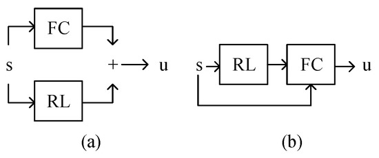
Figure 1.
Combination of FC and RL: (a) the parallel model. (b) The serial model.
In this paper, the serial controller of the terminal sliding mode control (TSMC) [21] and proximal policy optimization algorithms (PPO) [22] is proposed to solve the balance control task of RWBR while driving on curved pavements. The control problem considers matched disturbances (the dry friction of inertial wheel, etc.) and composite unmatched disturbances (including unmodeled wheel–ground contact, gust disturbances, and periodic disturbances induced by terrain, etc.). TSMC is a nonlinear FC method with strong robustness relative to system uncertainties and disturbances. PPO is a type of policy gradient training that alternates between sampling data via environmental interaction and optimizing a clipped surrogate objective function using stochastic gradient descent. With its excellent versatility and stability, it is used as a benchmark algorithm for RL at present. The proposed controller, called PPO-TSMC, explores the environment via output sampling with Gaussian distributions. The scalar value of the BR state quantity in disturbed environments is estimated by using a multi-layer neural network. The parameters of TSMC are tuned online by gradient descent under reasonable optimization objectives, and an adaptive terminal sliding mode controller based on RL is finally formed, which is used for the balance control of RWBR.
The contribution of this paper is to implement a PPO-TSMC controller that adaptively adjusts the parameters of TSMC online based on the RL method of PPO and to apply it to the balance control problem of RWBR while driving on a curved pavement. Specifically, a simplified numerical model of RWBR is derived, and a feedback transformation is designed for the simplified RWBR model. Then, a test scenario with multiple disturbances was constructed in MSC Adams, and the controller’s performances of RWBR using TSMC, adaptive integral terminal sliding mode (AITSM) [9], PPO, RRL, and PPO-TSMC were compared under different rear-wheel velocities and transverse periodic disturbance amplitudes of BR. The effectiveness and robustness of the proposed PPO-TSMC in task scenarios are verified. In addition, to the best knowledge of the authors, few studies considered the balance control of BR under both matched and unmatched disturbances on curved pavements.
This paper is organized as follows: The RWBR is described in Section 2, and a dynamical model referring to the inertial wheel pendulum is established using some assumptions and simplifications. In Section 3, the simplified dynamical model is transformed into chain form via feedback transformation. On this basis, the PPO-TSMC adaptive controller is designed. The TSMC Net., Critic Net., and the calculation flow of the adaptive adjustment of controller parameters are described in detail. In Section 4, the simulation environment in MSC Adams is built, and four test cases were designed; then, the performance of five different controllers are compared. Finally, in the Section 5, a conclusion is reached.
The video of the experiment is available at the following website: https://github.com/ZhuXianjinGitHub/PPO-TSMC, accessed on 25 October 2022.
2. Dynamics
In order to illustrate the motion of RWBR on a curved pavement, the reference frames are defined in Figure 2. The inertia frame is defined as , and the body-fixed reference frame is defined as , where the center is located at the center of gravity of the BR. The BR consists of four rigid bodies, namely, a rear wheel, body frame, reaction wheel, and front wheel (simplified as R, B, W, and F, respectively), as shown in Figure 2. In addition, the assumptions in the dynamical model are made as follows: (1) The thickness of the rear and front wheels is negligible, and the contacts between wheels and the ground are regarded as point contacts. (2) These four rigid bodies are symmetrical with respect to the plane of the rear and front wheels, so the center of mass of these bodies are in the same plane.
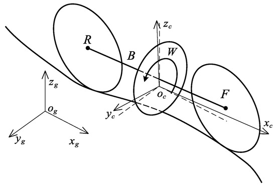
Figure 2.
RWBR on a curved pavement.
Consider the body frame and rear and front wheels as one unit P, and the reaction wheel as another W in Figure 3. The BR can be converted to an inertia wheel pendulum system [23]. The body fixed reference frames and are defined on P and W. The mass and inertia matrix of the two parts with respect to the body-fixed reference frame are , , , and . and represent the distance between the centroids of P and W and the connection between front- and rear-wheel ground points on a flat road:
where , , is the roll angle, is the reaction wheel angel, is the pitch angle of the robot, is the input torque of the reaction wheel’s motor, and and are mismatched/matched disturbances.
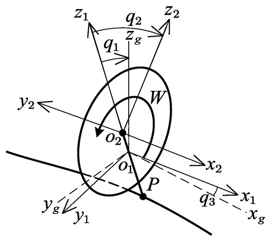
Figure 3.
Equivalent inertia wheel pendulum.
3. Design of Controller
First, the feedback transformation of an equivalent inertia wheel pendulum is introduced in this section. Upon this transformation, a terminal sliding mode controller is constructed. Then, the actor-critic framework, TSMC Net., and the key components of the PPO-TSMC are presented. The process and convergence of the PPO-TSMC are described. An analysis of the PPO optimization process for TSMC is performed.
3.1. Feedback Transformation and Terminal Sliding Mode Control
Feedback transformation is a common approach in the control of the nonlinear systems. Based on the Olfati-Saber transformation mentioned in [24,25], the following state variables and feedback transformation are defined (1).
The system can be expressed as follows:
where is bounded.
The TSMC is designed according to the method in [26]. First, define the recursive sliding surfaces as follows:
where and the sign function [27] is defined as follows:
and . Next, based on the sliding surfaces (5), the following output of the mean part of the TSMC Net. is defined as follows:
where and are the equivalent and reaching controllers with the following expressions:
where and , .
3.2. PPO-TSMC
In order to adopt reinforcement learning to optimize the TSMC, the above system needs to be discretized and meets the following assumptions.
Assumption 1.
The above system satisfies the Markov property, which means that the state at time t only depends on the state at the time and the corresponding action, independent of other historical states and inputs.
The actor-critic framework for the optimization of a Markov decision process includes two time-scale algorithms in which the critic uses temporal difference learning with a linear approximation architecture, and the actor is updated in an approximate gradient direction based on information provided by the critic. The actor-critic framework combined the advantages of actor-only and critic-only methods. PPO with the actor-critic style is one of the most popular on-policy RL algorithms. It simultaneously optimizes a stochastic policy as well as an approximator for the neural network value function. The main reason for choosing PPO in PPO-TSMC is that PPO uses conservative policy iterations based on an estimator of the advantage function to guarantee the monotonic improvement for general stochastic policies. The monotonic improvement guarantee for general stochastic policies can be found in [28].
PPO-TSMC aims at combing the interference rejection ability of TSMC and the monotonic improvement ablity of PPO. Specifically, in order to adaptively adjust the coefficients of TSMC using automatic differential software, the TSMC controller is represented as a neural network. The weights of the neural networks represent the coefficients of the TSMC. Then, the TSMC controller represented by a neural network is used to replace the mean part of the PPO’s actor network. Finally, the optimization framework based on PPO with an actor-critic is explored to adaptively adjust the coefficients of TSMC.
Remark 1.
In this paper, the reinforcement learning method is introduced to tune parameters , and θ of the TSMC controller (7)–(8). The main motivation of the PPO-TSMC control scheme is to improve the robustness with respect to matched and mismatched disturbances. Indeed, the online adaptation of can attenuate the matched disturbance , and well-adjusted parameters such as , and can lead to a more robust sliding surfaces against mismatched disturbance . The adaptive terminal sliding mode was also designed for RWBR in [9] , but the existing method only considered the online regulation of , so this method cannot actively compensate mismatched disturbances. Moreover, the adaptive gains of [9] are monotonic, which may cause more serious chattering in practice.
TSMC Net. (Figure 4) is used to map states to actions , in which represents the parameters of the policy . In this paper, strategy is a normal distribution comprising the mean part of TSMC and the standard deviation part of a non-negative output from a neural network.
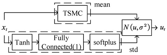
Figure 4.
TSMC Net.
The mean part: From the literature [24,29], state in (4) is the generalized momentum conjugate relative to in (1). Therefore, the control objective of RWBR can be equivalently considered as the stabilization of the transformed system (4).
The standard deviation part: The value of the standard deviation is output by the neural network, as shown in Figure 4. The structure of the neural network is set up by a hyperbolic tangent function , a fully connected layer, and a softplus activation function . The fully connected in Figure 4 represents the fully connected layer and i represents the number of neurons in the neural network. The weights of the neural network are independent of the states, such as the methods in [22].
The output of the TSMC Net. is as follows:
where denotes the weights of the neural network in the standard deviation part. represents adjustable parameters.
Remark 2.
The normal distribution can be seen as a diagonal Gaussian policy with one dimension. The Gaussian policy is one of the most common type of stochastic policies in deep RL and a type of policy used in continuous action space. The standard deviation in Gaussian policies controls the exploratory behavior during policy training. Different implementations of the standard deviation are discussed in [30].
The critic Net. implements a value function approximator that is used to map state to scalar value , in which means the parameter in the critic Net. The scalar value represents the predicted discounted cumulative long-term reward when the agent starts from the given state and takes the best possible action. The critic Net. of this paper is shown in Figure 5, which is composed of a deep neural network and an ReLU [31] nonlinear activation function. The gradient descent calculation of the critic Net. is shown in the next section.
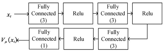
Figure 5.
Critic Net.
To facilitate the description of the composition and calculation process of PPO-TMSC, the framework of PPO-TSMC is shown in Figure 6. The process can be divided into three steps. In the first step, Gaussian noise is added on the output of the TSMC so that the RWBR can conduct some interactive exploration with the environment. The second step is to randomly sample the stored state and action sequence. The state value and advantage function under the finite-horizon estimators are calculated, and the parameters in critic Net. are updated. The third step is to update TSMC coefficients based on the information provided by critic Net.
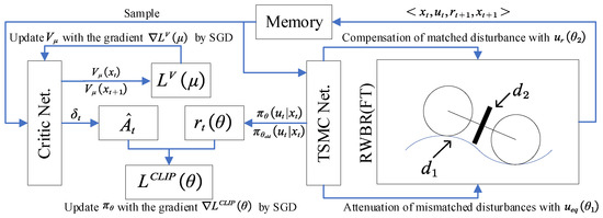
Figure 6.
The framework of the PPO-TSMC.
Step 1: can be obtained from the interaction of RWBR and the environment, can be calculated by transformation (2), is based on strategy (10), and the actual output of the controller can be obtained by the transformation (3). Then, and can be obtained by interactions with the environment. Reward can be calculated by (11). Then, is stored as tuples:
where and .
Step 2: Sample from the stored tuples and update the parameters of the critic Net. Sample a sequence of N tuples . The generalized advantage estimator (GAE) shown by (13) is estimated based on temporal difference errors :
where is the discounted factor for future rewards and is the smoothing factor for GAE. GAE (13) is beneficial for obtaining a better balance between bias and variance [32]. Update critic parameters by minimizing loss across all sampled mini-batch data:
where is the learning rate of critic Net.
Step 3: Update TSMC Net. by minimizing the loss function :
where represents the probability of taking action for a given state x, represents the corresponding probability of policy parameter before updates, and the clip ensures that each update will not fluctuate too much. is the entropy loss that is used to encourage the agent’s exploration, is the entropy loss weight factor, and represents the learning rate of TSMC Net.
Remark 3.
The global convergence proof for PPO is challenging since it uses deep neural networks, policies that become greedy, and previous policies for the trust region method. The authors of [33] provided an overview of a convergence proof. In [34], the two-time-scale stochastic approximation theory was employed to prove that PPO guarantees local convergence.
In TSMC-PPO, and can be ensured in the TSMC Net. The local convergence of PPO can ensure that the number of approaches 0. Therefore, the asymptotically stable TSMC-PPO can be guaranteed in practice.
4. Simulation Experiment
4.1. Simulation Platform
In order to verify the performance of the controller proposed in this paper, the simulation environment is built in MSC Adams, as shown in Figure 7.
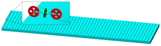
Figure 7.
RWBR on the curved pavement in MSC Adams.
In the simulation environment, an RWBR is placed on a curved pavement. According to the physical parameters of the BR, the parameters in Formula (1) are calculated as follows: kg, kg , kg, kg , and m. The maximum length of the robot is m. The function relationship between the height of the curved pavement and the direction of the of the inertia frame is , and the total length of the pavement is 60 m.
In MSC Adams, the contact force model includes the normal positive pressure based on collision [35] and the tangential friction force model based on velocity [36]. The function expression of collision positive pressure is listed as follows:
where is the penetration depth, k is the contact stiffness coefficient, e is force exponent, and d is the penetration depth when damping reaches the maximum. is the maximum damping coefficient. As shown in the Figure 8, the collision force has two parameters, the stiffness coefficient and the damping coefficient. Thus, the collision model can be used when assuming that the tire and the ground are made of rubber.
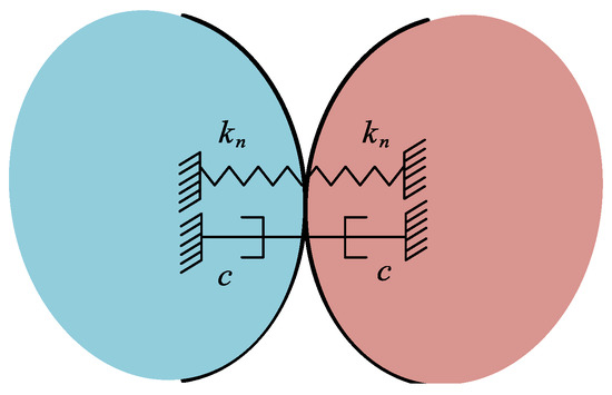
Figure 8.
Normal contact force model in MSC Adams.
As shown in Figure 9, the frictional force model based on velocity defined in (20) is an effective method for calculating tangential contact forces:
where is the relative velocity of contact points, and represent the stiction transition velocity and friction transition velocity, respectively, and and represent the static friction coefficient and dynamic friction coefficient, respectively.
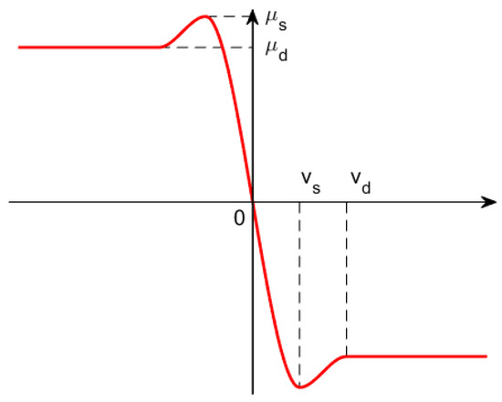
Figure 9.
Coefficient of friction in velocity-based friction model.
The step function expression in MSC Adams is defined as follows:
where , .
The parameters used in the contact force model can be chosen while following the instruction of previous studies [37,38], which provide recommended ranges of the related parameters for different materials. Based on those recommendations, the values of parameters are finally determined after multiple simulations in Adams.
Four test cases are formed by the combination of different rear-wheel angle velocities, v, and periodic lateral disturbances (for simulating wind gusts), d, as shown in Table 1. In addition, a vertical upward perturbation is added at the center of the RWBR.

Table 1.
The parameters of four test cases.
In each case, performances of TSMC, AITSM, PPO, RRL, and PPO-TSMC are compared. In all cases, the control frequency is set to 1 kHz. All cases in the experiments are set to 400 s. The initial coefficients of all controllers are tuned to obtain an acceptable control performance. Four existing controllers are implemented as follows. (1) The implementation of TSMC is shown in Section 3.1 in addition to parameters and . (2) PPO is implemented by replacing the TSMC Net. in Section 3.2 with the actor Net. The actor Net. in PPO is shown in Figure 10. (3) The output of the RRL is the output of TSMC multiplied by 0.7 plus the output of PPO multiplied by 0.3, as shown in Figure 1a. (4) The implementation of the AITSM controller is as follows:
and , and are generated by the adaptation laws as follows:
where , and .
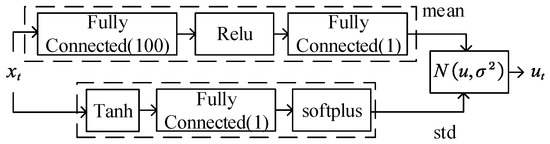
Figure 10.
Actor Net.
4.2. Experimental Results
In this section, we present the experimental results of the controllers, including TSMC, AITSM, RRL, RL, and PPO-TSMC. The following conclusions can be drawn from experiments. Firstly, the RWBR with PPO-TSMC is the only controller that completes the full 400 s test scenario in all four cases (Figure 11), which shows that it has the best robustness over others. Secondly, it is straightforward to observe that the PPO-TSMC obtained the smallest roll angle tracking error from Table 2; thus, PPO-TSMC has the best control performance among the five controllers. This is mainly due to the fact that both TSMCs without information about the bound of disturbance and AITSM with a monotonically increasing adaptation law (23) cannot maintain a good control performance for the balance control of RWBR with matched disturbances, mismatched disturbances, and unmodeled characteristics. Moreover, the reinforcement learning method is difficult to directly apply to the online balance control task. In order to adaptively adjust the parameters of TSMC, PPO-TSMC explores the influence of various disturbances through TSMC Net. and then fits an estimator of value function through a sequence of states, actions, and rewards. This value function can effectively guide the update of policy parameters based on gradients.
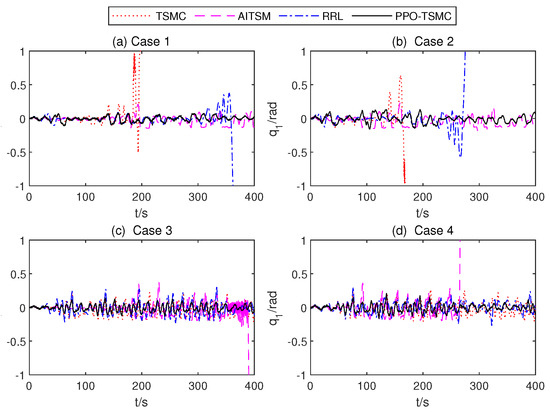
Figure 11.
Roll anglesof four different controllers.
Table 2.
Performance comparisons of five controllers.
Since the RWBR with RL easily falls, to rule out this low-efficiency controller, Figure 11 only presents the tracking performance of the remaining four controllers. Figure 12, Figure 13 and Figure 14 illustrate the variety of critic Net., weights, the mean parameters of the TSMC Net., and the std of TSMC Net. The gain value of AITSM is shown in Figure 15. In case 1 and case 2, the RWBR with the TSMC controller falls down in less than 200 s, and the RWBR with the RRL controller falls down at about 380 s and 300 s. In case 3 and case 4, the RWBR with the AITSM controller falls down at 390 s and 260 s, respectively. The RWBR with a PPO-TSMC controller completed 400 s simulation in all four cases.
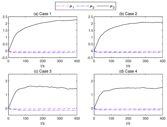
Figure 12.
Weights of one of the fully connected layers of the critic Net.
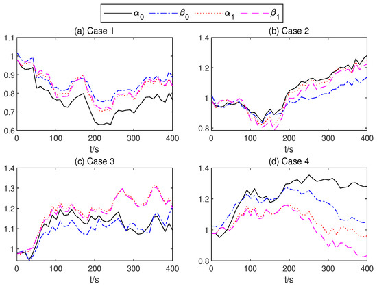
Figure 13.
of the mean part of the TSMC Net.
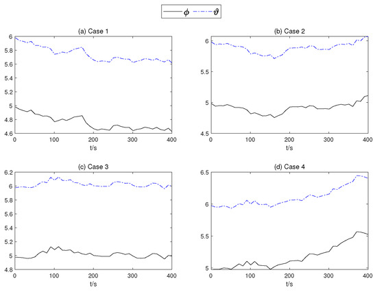
Figure 14.
of the mean part of the TSMC Net.
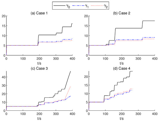
Figure 15.
The gain values of the AITSM.
In order to present the adaptive change process of the parameters of the proposed controller. In Figure 12, neural network weights of the middle layer of Critic Net. in four cases are described over time. As can be seen from Figure 12, at about 200 s, the weight of the Critic N. neural network becomes stable. In Figure 13 and Figure 14, the weight of TSMC Net, namely the coefficient of the sliding mode control, shows a relatively clear trend with respect to changes after 200 s. The adaptive parameter tunement method of AITSM (Figure 15) leads to the phenomenon of high-amplitude chattering, or even instability in Figure 11c, due to the monotonically increasing adaptation law (23).
For further data comparisons, the maximum (MAX), the root mean square (RMS), and the mean (MEAN) values of the roll are adopted, which are defined as follows.
In Table 2, for the BR that fell in the 400 s simulation test, no relevant comparisons were made between the system and the machine. The comparison of control performances under five controllers in four cases is listed. The simulations with PPO-TSMC exhibit the smallest MAX, MEAN, and RMS. The PPO controller behaves the worst performance. Although the TSMC controller can run the entire distance in case 1 and case 4, it performs poorly in case 1 and case 2, while AITSM and RRL controllers are better than TSMC but still worse than the proposed control. It can be concluded that the proposed PPO-TSMC controller achieves superior balancing performances compared to the other four proposed controllers.
5. Conclusions
In this paper, a PPO-TSMC controller is developed for the balancing purpose of an RWBR system on curved pavement with matched disturbances (the dry friction of inertia wheels, etc.) and composite mismatched disturbances (including unmodeled wheel–ground contact and gust disturbances and topographically introduced periodic disturbances, etc.). By connecting PPO and TSMC in series, a random action strategy based on a normal distribution is constructed in the framework of an initial TSMC controller. The controller parameters under disturbances and unmodeled characteristics are explored by using the strategy, and the online adaptive adjustment of TSMC parameters based on PPO algorithm is realized. The comparison between the proposed PPO-TSMC and TSMC, PPO, AITSM, and RRL illustrates stronger robustness and better control performance.
This study is different from existing related research studies about the reaction wheel bicycle robot from the perspective of the task, the method of the control, and the simulation test. Previous studies have not considered the influence of an unstructured curved pavement on the balance control of RWBR. For example, in [9] (2021), an adaptive integral terminal sliding mode control scheme was developed for the balancing purpose of the RWBR on a flat road with uncertainties and unmodelled dynamics by designing adaptive laws. In [39] (2022), an extreme-learning-machine scheme was designed as a compensator for estimating lumped uncertainties of the RWBR on a flat road. From the perspective of control methods, the existing studies [9,39] only considered reducing the influence of matched disturbances but not mismatched disturbances. However, not only the matched perturbation term but also the influence of the mismatched disturbances are considered in this work. Namely, parameters of the sliding mode surface and reaching control are adjusted simultaneously. In terms of simulation test settings, this work sets four different test cases in MSC Adams via different vehicle speeds and lateral disturbances. The comparison between the proposed PPO-TSMC and TSMC, PPO, AITSM, and RRL illustrates stronger robustness and better control performances. It shows that the PPO-TSMC in this work has application prospects.
On the other hand, improving the sample efficiency of the proposed PPO-TSMC will be considered as the main future research direction of this paper. From Figure 12 and Figure 13, the critic network does not become stable until about 200 s. Moreover, the convergence of actor Net. occurs later than that of critic Net. It is not very ideal for the practicability of the algorithm and limits the effectiveness of PPO-TSMC in a rapidly changing environment or when there are more random disturbances. Therefore, our future work aims to replace the critic deep neural network with Gaussian process regression [40], radial basis functions [41], or some other components of model-based reinforcement learning [42] to reduce the demand for data samples. Next, discretizing the output of the controller [43] is another method for reducing sample requirements. Finally, a physical deployment and pilot study are planned.
Author Contributions
Conceptualization, X.Z. (Xianjin Zhu); methodology, X.Z. (Xianjin Zhu); software, X.Z. (Xianjin Zhu) and X.Z. (Xudong Zheng); validation, X.Z. (Xianjin Zhu), Q.Z., Y.D. and X.Z. (Xudong Zheng); writing—original draft preparation, X.Z. (Xianjin Zhu); writing—review and editing, Y.D.; visualization, Q.Z.; supervision, Y.L.; project administration, Y.L. and B.L.; funding acquisition, B.L. and Y.D. All authors have read and agreed to the published version of the manuscript.
Funding
This research was funded by the National Natural Science Foundation of China (62203252).
Institutional Review Board Statement
Not applicable.
Informed Consent Statement
Not applicable.
Data Availability Statement
Not applicable.
Conflicts of Interest
The authors declare no conflict of interest.
References
- Stasinopoulos, S.; Zhao, M.; Zhong, Y. Simultaneous localization and mapping for autonomous bicycles. Int. J. Adv. Robot. Syst. 2017, 14, 172988141770717. [Google Scholar] [CrossRef]
- Zhang, Y.; Li, J.; Yi, J.; Song, D. Balance control and analysis of stationary riderless motorcycles. In Proceedings of the 2011 IEEE International Conference on Robotics and Automation (ICRA), Shanghai, China, 9–13 May 2011. [Google Scholar]
- Yu, Y.; Zhao, M. Steering control for autonomously balancing bicycle at low speed. In Proceedings of the 2018 IEEE International Conference on Robotics and Biomimetics (ROBIO), Kuala Lumpur, Malaysia, 12–15 December 2018. [Google Scholar]
- Sun, Y.; Zhao, M.; Wang, B.; Zheng, X.; Liang, B. Polynomial controller for BR based on nonlinear descriptor system. In Proceedings of the IECON 2020—46th Annual Conference of the IEEE Industrial Electronics Society, Singapore, 18–21 October 2020. [Google Scholar]
- Chen, C.K.; Chu, T.D.; Zhang, X.D. Modeling and control of an active stabilizing assistant system for a bicycle. Sensors 2019, 19, 248. [Google Scholar] [CrossRef] [PubMed]
- Zheng, X.; Zhu, X.; Chen, Z.; Sun, Y.; Liang, B.; Wang, T. Dynamic modeling of an unmanned motorcycle and combined balance control with both steering and double cmgs. Mech. Mach. Theory 2022, 169, 104–643. [Google Scholar] [CrossRef]
- He, K.; Deng, Y.; Wang, G.; Sun, X.; Sun, Y.; Chen, Z. Learning-Based Trajectory Tracking and Balance Control for BRs with a Pendulum: A Gaussian Process Approach. IEEE/ASME Trans. Mechatronics 2022, 27, 634–644. [Google Scholar] [CrossRef]
- Kim, Y.; Kim, H.; Lee, J. Stable control of the BR on a curved path by using a reaction wheel. J. Mech. Sci. Technol. 2015, 29, 2219–2226. [Google Scholar] [CrossRef]
- Chen, L.; Liu, J.; Wang, H.; Hu, Y.; Zheng, X.; Ye, M.; Zhang, J. Robust control of reaction wheel BR via adaptive integral terminal sliding mode. Nonlinear Dyn. 2021, 104, 291–2302. [Google Scholar]
- Kim, H.-W.; An, J.-W.; Yoo, H.d.; Lee, J.-M. Balancing control of bicycle robot using pid control. In Proceedings of the 2013 13th International Conference on Control, Automation and Systems (ICCAS 2013), Las Vegas, NV, USA, 24 October 2020–24 January 2021; pp. 145–147. [Google Scholar]
- Kanjanawanishkul, K. Lqr and mpc controller design and comparison for a stationary self-balancing BR with a reaction wheel. Kybernetika 2015, 51, 173–191. [Google Scholar]
- Owczarkowski, A.; Horla, D.; Zietkiewicz, J. Introduction of feedback linearization to robust lqr and lqi control—Analysis of results from an unmanned BR with reaction wheel. Asian J. Control. 2019, 21, 1028–1040. [Google Scholar] [CrossRef]
- Yi, J.; Song, D.; Levandowski, A.; Jayasuriya, S. Trajectory tracking and balance stabilization control of autonomous motorcycles. In Proceedings of the 2006 IEEE International Conference on Robotics and Automation, ICRA 2006, Orlando, FL, USA, 15–19 May 2006; pp. 2583–2589. [Google Scholar]
- Hwang, C.-L.; Wu, H.-M.; Shih, C.-L. Fuzzy sliding-mode underactuated control for autonomous dynamic balance of an electrical bicycle. IEEE Trans. Control. Syst. Technol. 2009, 17, 658–670. [Google Scholar] [CrossRef]
- Mnih, V.; Kavukcuoglu, K.; Silver, D.; Rusu, A.A.; Veness, J.; Bellemare, M.G.; Graves, A.; Riedmiller, M.; Fidjeland, A.K.; Ostrovski, G.; et al. Human-level control through deep reinforcement learning. Nature 2015, 518, 529–533. [Google Scholar] [CrossRef]
- Aradi, S. Survey of deep reinforcement learning for motion planning of autonomous vehicles. IEEE Trans. Intell. Transp. Syst. 2022, 23, 740–759. [Google Scholar] [CrossRef]
- Randløv, J.; Alstrøm, P. Learning to Drive a Bicycle Using Reinforcement Learning and Shaping; ICML: Baltimore, MD, USA, 1998. [Google Scholar]
- Choi, S.Y.; Le, T.; Nguyen, Q.; Layek, M.; Lee, S.G.; Chung, T.C. Toward self-driving bicycles using state-of-the-art deep reinforcement learning algorithms. Symmetry 2019, 11, 290. [Google Scholar] [CrossRef]
- Zheng, Q.; Wang, D.; Chen, Z.; Sun, Y.; Liang, B. Continuous reinforcement learning based ramp jump control for single-track two-wheeled robots. Trans. Inst. Meas. Control. 2022, 44, 892–904. [Google Scholar] [CrossRef]
- Johannink, T.; Bahl, S.; Nair, A.; Luo, J.; Kumar, A.; Loskyll, M.; Ojea, J.A.; Solowjow, E.; Levine, S. Residual reinforcement learning for robot control. In Proceedings of the 2019 International Conference on Robotics and Automation (ICRA), Montreal, QC, Canada, 20–24 May 2019; pp. 6023–6029. [Google Scholar]
- Venkataraman, S.; Gulati, S. Terminal sliding modes: A new approach to nonlinear control synthesis. In Proceedings of the 5th International Conference on Advanced Robotics ’Robots in Unstructured Environments, Pisa, Italy, 19–22 June 1991; Volume 1, pp. 443–448. [Google Scholar]
- Schulman, J.; Wolski, F.; Dhariwal, P.; Radford, A.; Klimov, O. Proximal policy optimization algorithms. arXiv 2017, arXiv:1707.06347. [Google Scholar]
- Olfati-Saber, R. Global stabilization of a flat underactuated system: The inertia wheel pendulum. In Proceedings of the IEEE Conference on Decision and Control, Los Alamitos, CA, USA, 4–7 December 2001; Volume 4, pp. 3764–3765. [Google Scholar]
- Olfati-Saber, R. Nonlinear Control of Underactuated Mechanical Systems with Application to Robotics and Aerospace Vehicles. Ph.D. Thesis, Massachusetts Institute of Technology, Cambridge, MA, USA, 2001. [Google Scholar]
- Spong, M.W.; Corke, P.; Lozano, R. Nonlinear control of the reaction wheel pendulum. Automatica 2001, 37, 1845–1851. [Google Scholar] [CrossRef]
- Zhou, M.; Feng, Y.; Han, F. Continuous full-order terminal sliding mode control for a class of nonlinear systems. In Proceedings of the 2017 36th Chinese Control Conference (CCC), Dalian, China, 26–28 July 2017; IEEE: Piscataway, NJ, USA, 2017; pp. 3657–3660. [Google Scholar]
- Shtessel, Y.; Edwards, C.; Fridman, L.; Levant, A. Sliding Mode Control and Observation; Publishing House: New York, NY, USA, 2014. [Google Scholar]
- Schulman, J.; Levine, S.; Abbeel, P.; Jordan, M.; Moritz, P. Trust region policy optimization. In Proceedings of the International Conference on Machine Learning, PMLR, Lille, France, 7–9 July 2015; pp. 1889–1897. [Google Scholar]
- Olfati-Saber, R. Normal forms for underactuated mechanical systems with symmetry. IEEE Trans. Autom. Control. 2002, 47, 305–308. [Google Scholar] [CrossRef]
- Andrychowicz, M.; Raichuk, A.; Stańczyk, P.; Orsini, M.; Girgin, S.; Marinier, R.; Hussenot, L.; Geist, M.; Pietquin, O.; Michalski, M.; et al. What matters in on-policy reinforcement learning? A large-scale empirical study. arXiv 2020, arXiv:2006.05990. [Google Scholar]
- Hinton, G.E. Rectified Linear Units Improve Restricted Boltzmann Machines Vinod Nair; ICML: Baltimore, MA, USA, 2010. [Google Scholar]
- Schulman, J.; Moritz, P.; Levine, S.; Jordan, M.; Abbeel, P. High-dimensional continuous control using generalized advantage estimation. arXiv 2015, arXiv:1506.02438. [Google Scholar]
- Konda, V.; Tsitsiklis, J. Actor-critic algorithms. In Proceedings of the Neural Information Processing Systems (NIPS), Denver, CO, USA, 29 November 29–4 December 1999. [Google Scholar]
- Holzleitner, M.; Gruber, L.; Arjona-Medina, J.; Brandstetter, J.; Hochreiter, S. Convergence proof for actor-critic methods applied to ppo and rudder. In Transactions on Large-Scale Data-and Knowledge-Centered Systems XLVIII; Springer: Berlin/Heidelberg, Germany, 2021; pp. 105–130. [Google Scholar]
- Machado, M.; Moreira, P.; Flores, P.; Lankarani, H.M. Compliant contact force models in multibody dynamics: Evolution of the hertz contact theory. Mech. Mach. Theory 2012, 53, 99–121. [Google Scholar] [CrossRef]
- Marques, F.; Flores, P.; Claro, J.P.; Lankarani, H.M. A survey and comparison of several friction force models for dynamic analysis of multibody mechanical systems. Nonlinear Dyn. 2016, 86, 1407–1443. [Google Scholar] [CrossRef]
- Giesbers, J. Contact Mechanics in MSC Adams-a Technical Evaluation of the Contact Models in Multibody Dynamics Software MSC Adams. Ph.D. Thesis, University of Twente, Twente, The Netherlands, 2012. [Google Scholar]
- Sapietová, A.; Gajdoš, L.; Dekỳxsx, V.; Sapieta, M. Analysis of the influence of input function contact parameters of the impact force process in the msc. adams. In Advanced Mechatronics Solutions; Springer: Berlin/Heidelberg, Germany, 2016; pp. 243–253. [Google Scholar]
- Chen, L.; Yan, B.; Wang, H.; Shao, K.; Kurniawan, E.; Wang, G. Extreme-learning-machine-based robust integral terminal sliding mode control of bicycle robot. Control. Eng. Pract. 2022, 124, 105064. [Google Scholar] [CrossRef]
- Deisenroth, M.P.; Fox, D.; Rasmussen, C.E. Gaussian processes for data-efficient learning in robotics and control. IEEE Trans. Pattern Anal. Mach. Intell. 2013, 37, 408–423. [Google Scholar] [CrossRef] [PubMed]
- Chettibi, T. Smooth point-to-point trajectory planning for robot manipulators by using radial basis functions. Robotica 2019, 37, 539–559. [Google Scholar] [CrossRef]
- Moerl, T.M.; Broekens, J.; Jonker, C.M. Model-based reinforcement learning: A survey. arXiv 2020, arXiv:2006.16712. [Google Scholar]
- Rietsch, S.; Huang, S.Y.; Kontes, G.; Plinge, A.; Mutschler, C. Driver Dojo: A Benchmark for Generalizable Reinforcement Learning for Autonomous Driving. arXiv 2022, arXiv:2207.11432. [Google Scholar]


Publisher’s Note: MDPI stays neutral with regard to jurisdictional claims in published maps and institutional affiliations. |
© 2022 by the authors. Licensee MDPI, Basel, Switzerland. This article is an open access article distributed under the terms and conditions of the Creative Commons Attribution (CC BY) license (https://creativecommons.org/licenses/by/4.0/).