A Time-Varying PD Sliding Mode Control Method for the Container Crane Based on a Radial-Spring Damper

Abstract

For the multi-rope structure of the container crane system and its large mass payload anti-swing positioning problem, an equivalent double-swing model based on radial spring-dampers is established and a time-varying PD sliding mode controller (TVPD-SMC) with improved transient performance is proposed. In particular, the dynamics of the container crane system are first analyzed using the Lagrange method, and an equivalent double pendulum dynamics model of the crane is established. Compared with the traditional double pendulum model, this model ensures the accuracy of modeling without measuring the second pendulum angle. On this basis, an enhanced coupled time-varying sliding mode control method is designed to eliminate the sliding mode control method’s reaching phase and improves the robustness of the controller. Finally, the convergence and stability of the closed-loop system are proved using the Lyapunov technique and the Lasalle invariance theorem, and the simulation results demonstrate the effectiveness of the method.

1. Introduction

Container cranes are widely used in the industrial field for their advantages of high work efficiency, high positioning accuracy, and convenient transportation. For the container crane system, on the one hand, the need to quickly and accurately achieve the “point-to-point” transportation of goods; on the other hand, the cargo swing in the transport process must be suppressed in a small range to ensure operational safety. However, due to the underactuated characteristics of the crane system, it is highly susceptible to large payload swing during transportation due to the unmodeled dynamics of the system and external disturbances, thus seriously affecting the positioning accuracy and safety of the system. Therefore, in order to solve these problems, researchers have conducted in-depth studies mainly on two aspects: dynamics modeling and controller design of cranes [1,2].

From the point of view of dynamics modeling, less research has been done on container cranes compared to single-rope cranes [3]. Since it is difficult to further analyze the multi-rope structure of container cranes, existing studies commonly equate their multi-rope structures to single-rope structures before modeling the dynamics, but this method reduces the accuracy of the dynamics model [4,5]. Therefore, to improve the accuracy of dynamics modeling, a number of scholars have studied and analyzed the multi-rope structure of container cranes in recent years [6,7,8,9,10]. Xu et al. simplified the eight-link container crane to an inverted triangular linkage mechanism and experimentally verified that the model could describe the dynamics of the crane system to a certain extent [6]. Based on the idea that a more accurate model can improve controller response performance, Lu et al. proposed a new modeling technique to build an accurate model of a four-rope crane [7]. Unfortunately, these results do not consider the double pendulum effect generated by the container crane system and therefore do not provide a good description of the motion law of a crane system. To solve this problem, Masoud and Nayfeh developed a more accurate double pendulum model for multi-rope cranes and further constructed a delayed feedback controller based on it [10]. However, due to the limitation of the system structure, the second pendulum angle (the pendulum angle between the hook and the container) is often difficult to obtain by sensors in practical applications.

From the control point of view, for the two-dimensional multi-rope container crane system, the variables to be controlled are more than the amount of system control, which is an underactuated system, and the control problem of such a system is very challenging. To this end, many scholars have proposed a series of control methods, including input integer [11], trajectory planning [12], optimal control [13], adaptive control [14], robust control [15,16,17], and intelligent control [18,19]. Among them, sliding mode control as a robust control method (SMC) has high robustness and is insensitive to system parameters and external disturbances. Therefore, some scholars have applied the sliding mode control method to the container crane system [20,21,22,23,24]. Specifically, Bartolini proposed a second-order sliding mode control method for container cranes and experimentally verified the good control anti-swing positioning performance of the method [20]. To better tune the gain of sliding mode control, Quang combined sliding mode control with a fuzzy logic system and designed a new method for online adjustment of the linear sliding mode surface, proposing a fuzzy sliding mode controller which effectively reduces the chattering phenomenon of the sliding mode surface [22]. However, the system modeling error and parameter perturbation cause the controller to only maintain good performance under the set transport conditions. For this reason, Bessa designed an adaptive mechanism and proposed an adaptive fuzzy sliding mode controller based on it, thus effectively improving the adaptability of this controller to different working conditions [24]. Nevertheless, the existing sliding mode control method for multi-rope container cranes has two problems: first, the coupling between swing angle and displacement is not considered, and the transient performance is poor; second, there is a sliding mode reaching phase, which does not have global robustness.

To solve the above problems, this paper first promotes the previous modeling techniques and analyzes the multi-rope structure of container crane, then proposes an equivalent double pendulum container crane system dynamics model based on radial spring-dampers. On this basis, a time-varying PD sliding mode control method is designed with improved transient performance. The asymptotic stability of the expected equilibrium point is strictly guaranteed by using the Lyapunov technique and the Lasalle invariance theorem. Finally, extensive simulation experiments are conducted by MATLAB/Simulink to verify the feasibility and effectiveness of the method. The advantages of the method proposed in this paper are as follows:

(1)

Compared with the conventional double pendulum model, the proposed model in this paper does not need to measure the second pendulum angle, which reduces the difficulty of engineering applications and ensures the accuracy of the model;

(2)

The time-varying PD sliding mode controller proposed in this paper reduces the arrival time of the sliding mode surface, enhances the coupling between the system state quantities, has high global robustness and better transient performance, and is verified by simulation experiments;

(3)

In this paper, a new switching function is adopted to replace the original symbolic function, which effectively eliminates the chattering phenomenon of the sliding mode.

The rest of this paper is organized as follows: In Section 2, the method of establishing the equivalent double pendulum model of the container crane system based on radial spring-dampers is introduced, and the validity of the model is verified theoretically; in Section 3, the design process and stability proof of the time-varying PD sliding mode controller are introduced in detail; the simulation experimental results are provided in Section 4; finally, some concluding remarks are given in Section 5.

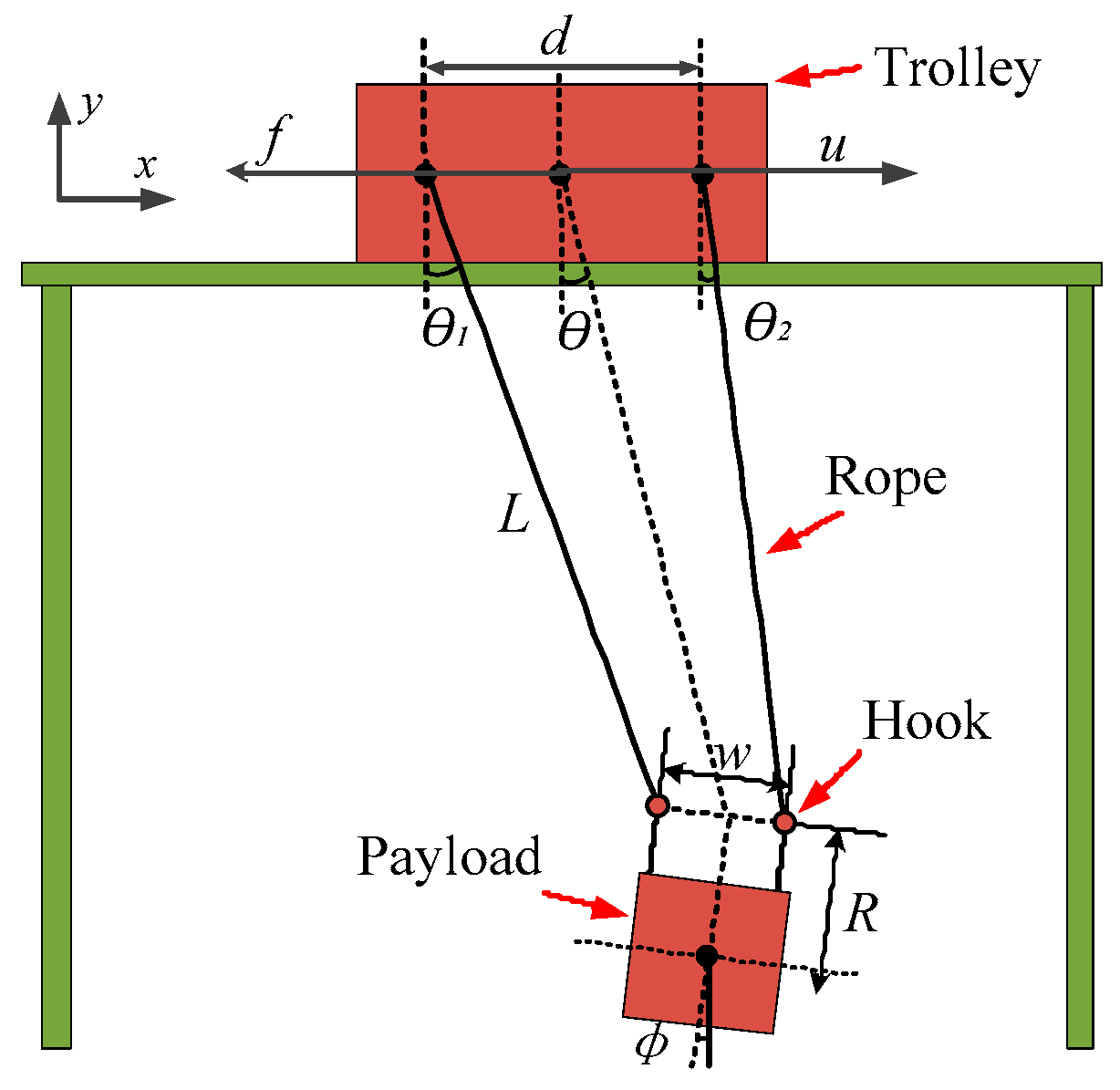
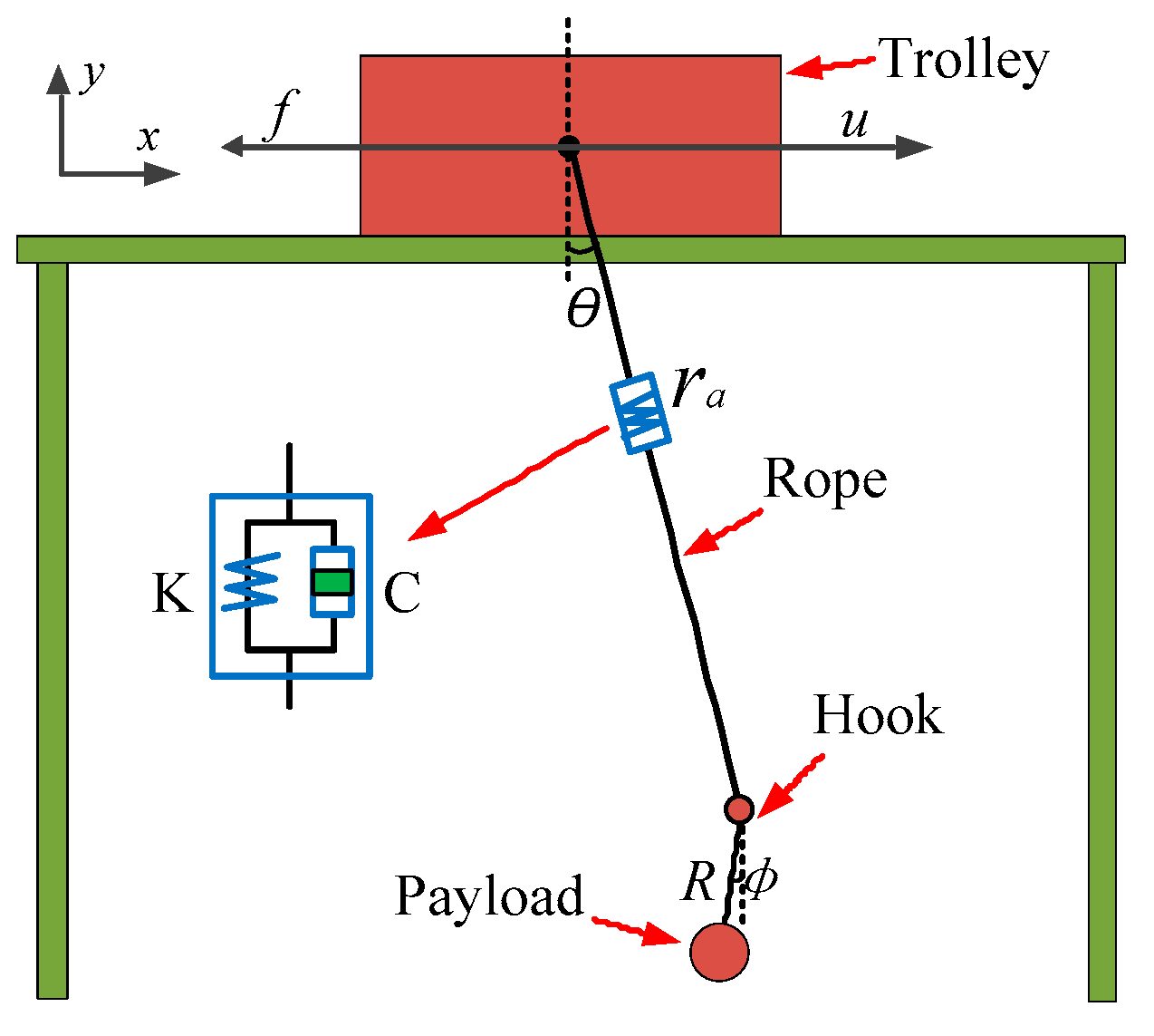
2. 2D Container Crane System Model

In this section, an equivalent double pendulum model based on radial spring-damper is proposed, and the validity of the model is tested. The two-dimensional model of the container crane system is shown in Figure 1.

Remark 1.

The masses of the lifting ropes are so negligibly small in comparison to the cargo that they can be disregarded. As a result, the ropes are considered as massless rigid bodies in this paper, as is frequently the case in works on cranes. Additionally, the two parts of the steel rope between the hook and the weight are of equal length, and the connection between the hook and the steel rope is fixed.

Remark 2.

For container cranes, the transport in the X- and Y-axis directions is a similar process and can be seen as two independent one-dimensional movements. In addition, the payload is only lifted at the starting and target positions, while there is no lifting motion during the transportation process. Since this paper mainly focuses on the control during payload transportation, its lifting motion is not considered. This simplification holds in most cases and is therefore widely adopted by other crane-related works. For example, literature [3,25,26]. The situations where such an assumption is not satisfied will be solved in the future work.

The hook, which is lifted by two steel ropes of equal length and attached to the crane, captures the weight during crane operation. According to Figure 1, the steel rope is spaced apart by d on the trolley and w on the hook, which satisfies the criterion that d > w; L is the steel rope length; and R is the distance between the payload and the hook barycenter. M, m₁ and m₂ represent the mass of trolley, hook and payload, respectively. ${\theta }_1\mathrm{and}{\theta }_2$ represent the swing angle of the sling, respectively. φ represents the swing of the payload with respect to the vertical direction. u is the driving force of the trolley, and f is the friction between the trolley and the guide rail. According to the literature [27], the constraint relation of each swing angle can be established and simplified, and the following can be obtained:

$$\{\begin{array}{l}L\sin {\theta }_1+w\cos \phi =d+L\sin {\theta }_2\\ L\cos {\theta }_1+w\sin \phi =L\cos {\theta }_2\end{array},$$

(1)

$$\phi =\frac{d-w}{w}\theta =a\theta .$$

(2)

According to the motion characteristics and constraints of the multi-rope container crane, it is considered to be the double pendulum model as shown in Figure 2 [10]. In addition, a radial spring-damped anti-swing device is designed by combining a spring oscillator and a dampener [28]. Figure 2 shows that θ stands for the angle between the trolley and the hook barycenter. r_a is the radial spring damper, where K and C represent the spring coefficient and damping coefficient, respectively. The payload will generate a radial tension in the direction of the rope during the motion, causing deformation of the spring oscillator with deformation variable r. The assumptions of the container crane system are described as follows [28]:

Assumption 1.

Ignore the mass of the radial spring-damper anti-swing device;

Assumption 2.

During the transportation process, the payload swing angles always remains in the interval between −π/2 and π/2, i.e.,

$$-\frac{\pi }{2}<\theta <\frac{\pi }{2},-\frac{\pi }{2}<\phi <\frac{\pi }{2}.$$

(3)

Assumption 3.

The steel rope distortion is disregarded, and its length L is considerably more than the spring-shaped variable r, specifically:

$$l_1>>r.$$

(4)

Remark 3.

In general, it is actually necessary and more accurate to model a container crane as a double pendulum. First of all, in practical applications, the presence of a hook or a large payload size will necessarily cause a double pendulum swing effect (DPSE) of the crane. The difference is that when the hook mass or payload is large, the DPSE will be more marked, and vice versa may be less distinct. According to a large number of practical applications, this DPSE cannot be ignored in many instances. On the other hand, the developed double pendulum model is actually a generalization of the traditional crane model. This is because the double pendulum crane model degenerates to a single pendulum model when the hook mass is zero. This fact further indicates that the results obtained from the double pendulum model are applicable to a wider range of crane systems [25].

Remark 4.

The Container Crane System considered is very different from the Double Pendulum Crane System of Le [29] and Zhang [26] for the following reasons: (1) the Container Crane System requires three angles to accurately describe the swing of the payload, while the Double Pendulum Crane System only requires two angles; (2) the pendulum angle of the Container Crane System is not independent, but is constrained by some geometric relationships, making its model more complex and internally coupled stronger; (3) the container crane system needs to consider the size and attitude of the payload, while the double pendulum crane system treats the payload as a mass point; (4) the practical applications of these two systems are different.

A rectangular coordinate system is created where the positive X-axis represents the direction of the driving force, the positive Y-axis is perpendicular to the ground downward, and the movement displacement of the trolley is represented by the letter x. The mass of trolley, hook and payload are M, m₁ and m₂, respectively. The bridge crane system model is established using generalized coordinates, with the truck, hook, and payload having the coordinates (X_M, Y_M), (x₁, y₁) and (x₂, y₂), respectively, as follows:

$$\{\begin{array}{l}{X}_{\mathrm{M}}=x\\ Y_{\mathrm{M}}=0\\ x_1=x+(L+r)\sin \theta \\ y_1=(L+r)\cos \theta \\ x_2=x+(L+r)\sin \theta -R\sin \phi \\ y_2=(L+r)\cos \theta +R\cos \phi \end{array}.$$

(5)

The total kinetic energy of bridge container crane system mainly includes trolley kinetic energy, hook kinetic energy and payload kinetic energy. The payload possesses rotating kinetic energy because it is a distributed mass affecting its moment of inertia from both translation and rotation. The overall potential energy of the system consists of the gravitational potential energy as well as the elastic potential energy of the spring-damper, assuming that the trolley plane has zero potential energy. In (6) and (7), respectively, specific expressions of kinetic energy and potential energy are displayed:

$$\begin{array}{l}{E}_k=\frac{1}{2}M\dot{x}+\frac{1}{2}{m}_1{(\dot{x}+L\cos \theta \dot{\theta }+\dot{r}\sin \theta +r\cos \theta \dot{\theta })}^2+\frac{1}{2}{m}_1(-L\sin \theta \dot{\theta }\\ +\dot{r}\cos \theta -r\sin \theta \dot{\theta }{)}^2+\frac{1}{2}{m}_2{(\dot{x}+L\cos \theta \dot{\theta }+\dot{r}\sin \theta +r\cos \theta \dot{\theta }-aR\cos a\theta \dot{\theta })}^2\\ +\frac{1}{2}{m}_2{(-L\sin \theta \dot{\theta }+\dot{r}\cos \theta -r\sin \theta \dot{\theta }-aR\sin a\theta \dot{\theta })}^2+E_w\end{array},$$

(6)

$$E_p=-m_{1}g(L+r)\cos \theta -m_{2}g(L+r)\cos \theta -m_{2}gR\cos a\theta +\frac{1}{2}K{r}^2,$$

(7)

where $E_w=\frac{1}{2}\mathrm{J}{\dot{\phi }}^2$ is the payload rotating kinetic energy. Lagrange equation is used to establish the dynamic equation of the crane system. Its general expression is as follows:

$$\frac{d}{dt}\left(\frac{\partial L}{\partial {\dot{q}}_k}\right)-\frac{\partial L}{\partial q_k}+\frac{\partial Q_c}{\partial {\dot{q}}_k}=F_k,$$

(8)

with $q_k$ representing the state variable, $\dot{q_k}$ meaning the first derivative of the state variable, k = 1, …, n (n represents the number of state quantities), Lagrange operator L representing the difference between the kinetic energy and the potential energy of the system, F_k representing the generalized force, and $Q_c=\frac{1}{2}C{\dot{r}}^2$ representing the dissipated energy of the damper. According to (6)–(8), using Lagrange modeling method in generalized coordinates, we obtain the following results of the crane dynamic equation:

$$\begin{array}{l}(M+m)\ddot{x}+[m{L}_r\cos \theta -m_{2}aR\cos (a\theta )]\ddot{\theta }+m\sin \theta \ddot{r}+2(m_1-m_2)\cos \theta \dot{\theta }\dot{r}\\ +(-m_1{L}_r\sin \theta \dot{\theta }+m_2(Ra\sin (a\theta )-L_r\sin \theta )){\dot{\theta }}^2=F_x-f\end{array},$$

(9)

$$\begin{array}{l}[m{L}_r\cos \theta -m_{2}aR\cos (a\theta )]\ddot{x}+(m{L}_r{}^2+m_2{a}^2{R}^2)\ddot{\theta }-m_{2}Ra\sin (a\theta +\theta )\ddot{r}\\ +m_2(LRa\sin (a\theta +\theta )\dot{\theta }+2a\dot{r}R\cos (a\theta +\theta ))\dot{\theta }+m_{1}g{L}_r\sin \theta +2m{L}_r\dot{\theta }\dot{r}\\ +m_2\sin (a\theta +\theta )(L_{r}R{a}^2+rRa)+m_2(g{L}_r\sin \theta +agR\sin (a\theta ))=0\end{array},$$

(10)

$$m\sin \theta \ddot{x}-m_{2}Ra\sin (a\theta +\theta )\ddot{\theta }+m\ddot{r}-(m{L}_r+m_2{a}^{2}R\cos (a\theta -\theta )){\dot{\theta }}^2+Kr=F_r-c\dot{r},$$

(11)

where m = m₁ + m_2, L_r = L + r. For the container crane system, the friction force is nonlinear and depends on its velocity. Therefore, the following friction model is selected in this paper [30]:

$$f=f_r\tanh \left(\dot{x}/{\epsilon }_x\right)-k_{rx}\left|\dot{x}\right|\dot{x},$$

(12)

with $f_r,{\epsilon }_x,k_{rx}\in {\mathrm{R}}^{+}$ being the friction-related parameters. For the convenience of subsequent analysis, the dynamic (9)–(11) are rewritten into a matrix form as follows:

$$\mathit{M}\left(\mathit{q}\right)\ddot{\mathit{q}}+\mathit{C}\left(\mathit{q},\dot{\mathit{q}}\right)\dot{\mathit{q}}+\mathit{G}\left(\mathit{q}\right)=\mathit{U}+{\mathit{d}}_{\mathit{f}},$$

(13)

$$\begin{array}{l}M=\left[\begin{array}{ccc}M+m& m{L}_r\cos \theta -m_{2}aR\cos (a\theta )& m\sin \theta \\ m{L}_r\cos \theta -m_{2}aR\cos (a\theta )& m{L}_r{}^2+m_2(a^2{R}^2-2aR{L}_r\cos (a\theta +\theta ))+J{a}^2& -m_{2}Ra\sin (a\theta +\theta )\\ m\sin \theta & -m_{2}Ra\sin (a\theta +\theta )& m\end{array}\right];\\ C=\left[\begin{array}{ccc}0& (-m{L}_r\sin \theta +m_{2}R{a}^2\sin (a\theta ))\dot{\theta }& 2(m_1-m_2)\cos \theta \dot{\theta }\\ 0& m_{2}Ra(L\sin (a\theta +\theta )\dot{\theta }+\sin (a\theta +\theta )(L_{r}a+r))& 2\dot{\theta }(m{L}_r-m_{2}aR\cos (a\theta +\theta ))\\ 0& -(m{L}_r+m_2{a}^{2}R\cos (a\theta -\theta ))\dot{\theta }& 0\end{array}\right];\\ G={\left[\begin{array}{ccc}0& mg{L}_r\sin \theta +m_{2}agR\sin (a\theta )& Kr-mg\cos \theta \end{array}\right]}^T;\\ F={\left[\begin{array}{ccc}{F}_x& F_{\theta }& F_r-c\dot{r}\end{array}\right]}^T;d_f={\left[\begin{array}{ccc}-f& 0& 0\end{array}\right]}^T;\end{array}.$$

(14)

The properties of the container crane system are described as follows [31]:

Property 1: M(q) is a positive definite symmetric matrix.

Property 2: $\dot{\mathit{M}}\left(\mathit{q}\right)/2-\mathit{C}\left(q,\dot{\mathit{q}}\right)$ is skew symmetric, i.e.,

$$\begin{array}{cc}{\mathit{\epsilon }}^T\left(\frac{\dot{\mathit{M}}\left(\mathit{q}\right)}{2}-\mathit{C}\left(\mathit{q},\dot{\mathit{q}}\right)\right)\mathit{\epsilon }=0,& \forall \mathit{\epsilon }\in R^4\end{array}.$$

(15)

According to (13), M(q) is the inertia matrix of the system, and M(q) > 0, which is consistent with Property 1. Container cranes strictly follow the law of conservation of energy in the process of transportation. According to (13), the kinetic energy of the system can be expressed as

$$E_k=\frac{1}{2}{\dot{\mathit{q}}}^T\mathit{M}\dot{\mathit{q}}.$$

(16)

Taking the derivative of (16), the first derivative of the kinetic energy of the system can be obtained as follows:

$$\dot{E}k={\dot{\mathit{q}}}^T(\mathit{M}\ddot{\mathit{q}}+\frac{1}{2}\dot{\mathit{M}}\dot{\mathit{q}}).$$

(17)

According to (13), the external force of the system can be obtained as U–G. According to the law of energy conservation and conversion, the work done by the external force will cause the change of kinetic energy of the system, so the following equation can be obtained:

$$\dot{E}k={\dot{\mathit{q}}}^T(\mathit{U}-\mathit{G}).$$

(18)

According to (13), (17) and (18):

$${\mathit{\epsilon }}^T\left(\frac{\dot{\mathit{M}}\left(\mathit{q}\right)}{2}-\mathit{C}\left(\mathit{q},\dot{\mathit{q}}\right)\right)\mathit{\epsilon }=0.$$

(19)

Equation (19) is consistent with Property 2 after comparison. The accuracy of the corresponding double-swing container crane model based on radial spring-damper is somewhat confirmed by examining the physical meaning of properties 1 and 2.

3. Controller Design and Stability Analysis

In this section, a time-varying PD sliding mode controller (TVPD-SMC) with improved transient performance is proposed. Furthermore, the asymptotic stability of the required equilibrium point is rigorously analyzed using the Lyapunov technique and the LaSalle invariance theorem.

3.1. TVPD-SMC Design

Enhancing the coupling behavior between trolley displacement x and payload swing angle θ will improve the control performance of an underactuated overhead crane. Therefore, a coupling signal as shown in (20) is introduced in this paper [32]. Its derivative with respect to time is shown in (21) and (22).

$${\xi }_x=x-\gamma {\displaystyle {\int }_0^t\theta }d\tau ,$$

(20)

$${\dot{\xi }}_x=\dot{x}-\gamma \theta ,$$

(21)

$${\ddot{\xi }}_x=\ddot{x}-\gamma \dot{\theta },$$

(22)

where γ ∈ R⁺ denotes the positive control parameter. Therefore, a new state variable can be obtained as shown in (23), and its derivative with respect to time is shown in (24). Based on (13) and (20)–(22), the kinetic equation can be written as shown in (25).

$$\mathit{\eta }(\mathit{t})={\left[\begin{array}{ccc}{\xi }_x& \theta & r\end{array}\right]}^T,$$

(23)

$$\begin{array}{l}\dot{\mathit{\eta }}(\mathit{t})={\left[\begin{array}{ccc}{\dot{\xi }}_x& \dot{\theta }& \dot{r}\end{array}\right]}^T\\ \ddot{\mathit{\eta }}(\mathit{t})={\left[\begin{array}{ccc}{\ddot{\xi }}_x& \ddot{\theta }& \ddot{r}\end{array}\right]}^T\end{array},$$

(24)

$$\begin{array}{c}\mathit{M}\ddot{\eta }+\mathit{C}\dot{\eta }+\mathit{G}+\mathit{Z}=\mathit{U}-{\mathit{d}}_{\mathit{f}};\\ \mathit{Z}={\left[\begin{array}{ccc}(M+m)({\gamma }_1\dot{\theta }+{\gamma }_2\dot{r})& m{L}_r\cos \theta -m_{2}aR\cos (a\theta )({\gamma }_1\dot{\theta }+{\gamma }_2\dot{r})& m\sin \theta ({\gamma }_1\dot{\theta }+{\gamma }_2\dot{r})\end{array}\right]}^{\mathrm{T}}\end{array}.$$

(25)

We define η_d = (x_d, 0, 0) as the target position, where x_d represents the target value of the trolley. To achieve the control objective, the error signal is defined as (26), and a time-varying sliding mode surface is designed as shown in (27).

$${\mathit{e}}_{\eta }=\eta -{\eta }_{\mathit{d}}={\left[\begin{array}{ccc}{\xi }_x-x_d& \theta & r\end{array}\right]}^T={\left[\begin{array}{ccc}{e}_{\xi }& \theta & r\end{array}\right]}^T,$$

(26)

$$\mathit{s}(t)={\dot{\mathit{e}}}_{\eta }+\beta {\mathit{e}}_{\eta }+\mathit{f}(t),$$

(27)

where β = diag [1,0,0] represents the sliding mode constant. Inspired by literature [33] and [34], a time-varying function is added to the sliding surface of this paper, which eliminates the reaching phase of the sliding mode and makes the controller globally robust. The detailed expression of this time-varying function is shown in Equation (28).

$$\mathit{f}(t)=\mathit{f}(0){\mathrm{e}}^{-\mu t},$$

(28)

where μ is the time-varying function gain. The time-varying function f(t) should satisfy the conditions shown in (29). The sliding mode control system is made globally robust to system parameter uncertainties and outside disturbances owing to the time-varying sliding mode feature.

$$\mathit{f}\left(0\right)=-{\dot{\mathit{e}}}_{\eta }(0)-\beta {\mathit{e}}_{\eta }(0)=\beta {\eta }_{\mathit{d}},\mathit{f}(\infty )=0.$$

(29)

For container crane system, a TVPD-SMC method is proposed:

$$F=\alpha (d_f+Z+G-M(\mathsf{\beta }{\dot{e}}_{\eta }+\dot{f}(t))-C(\mathsf{\beta }{e}_{\eta }+\mathrm{f}(t))-k_p{\displaystyle {\int }_0^{t}s}d\tau -k_{d}s-\mathsf{\lambda }\mathrm{sgn}(s)),$$

(30)

where k_p and k_d are proportional differential control gains, λ represents the sliding mode controller gain, α = [1,0,0] is the sliding mode controller constant. To overcome chattering in the switching process of sliding mode surface caused by the discontinuity of sign function, a continuous switching function is designed as shown in (31), so the control law is rewritten in the form of Equation (32).

$$th\left(s\right)=\{\begin{array}{l}1-\frac{2}{{\mathrm{e}}^2+1},s\ge 1\\ \frac{{\mathrm{e}}^s-{\mathrm{e}}^{-s}}{{\mathrm{e}}^s+{\mathrm{e}}^{-s}},\left|s\right|<1\\ -1+\frac{2}{{\mathrm{e}}^2+1},s\le -1\end{array},$$

(31)

$$F=\alpha ({\mathit{d}}_f+\mathit{Z}+\mathit{G}-\mathit{M}(\beta {\dot{\mathit{e}}}_{\eta }+\dot{\mathrm{f}}(t))-\mathit{C}(\beta {\mathit{e}}_{\eta }+\mathrm{f}(t))-{\mathit{k}}_p{\displaystyle {\int }_0^t\mathit{s}}d\tau -{\mathit{k}}_{d}s-\lambda \mathrm{th}(s)).$$

(32)

3.2. Stability Analysis

Theorem 1

: Under the TVPD-SMC method (32) proposed in this paper, the payload swing angle can be suppressed and eliminated while the trolley can reach the specified position, as shown in (33).

$$\underset{t\to \infty }{\lim }{\left(\begin{array}{ccc}x& \theta & \phi \end{array}\right)}^T={\left(\begin{array}{ccc}{x}_d& 0& 0\end{array}\right)}^T.$$

(33)

Proof . 

To prove Theorem 1, a positive Lyapunov candidate function inspired by the literature [27] was designed as shown in Equation (34).

$$\mathit{V}(t)=\frac{1}{2}{\mathit{s}}^T\mathit{M}\mathit{s}+\frac{1}{2}{k}_p{({\displaystyle {\int }_0^t\mathit{s}}d\tau )}^T({\displaystyle {\int }_0^t\mathit{s}}d\tau )+\left[\frac{\pi }{2}-\arctan \left({\displaystyle {\int }_0^t\left({\dot{\theta }}^2+{\dot{r}}^2\right)d\tau }\right)\right]{\alpha }^T.$$

(34)

In Equation (34), it is known that both $\frac{1}{2}{\mathit{s}}^{\mathrm{T}}\mathit{M}\mathit{s}$ and $\frac{1}{2}{k}_p{({\displaystyle {\int }_0^t\mathit{s}}d\tau )}^T({\displaystyle {\int }_0^t\mathit{s}}d\tau )$ are positive values according to the rules of matrix operations. Since $\arctan \left(x\right)\in \left[-\mathsf{\pi }/2,\mathsf{\pi }/2\right]$, the third component of the Lyapunov function, $\left[\frac{\pi }{2}-\arctan \left({\displaystyle {\int }_0^t\left({\dot{\theta }}^2+{\dot{r}}^2\right)d\tau }\right)\right]{\alpha }^T$, is a positive value. By taking the first derivative of (34) with respect to time, and substituting (27) and (32), we can obtain the following:

$$\begin{array}{l}\dot{\mathit{V}}(t)={\mathit{s}}^T\mathit{M}\dot{\mathit{s}}+\frac{1}{2}{\mathit{s}}^T\dot{\mathit{M}}\mathit{s}+k_p{({\displaystyle {\int }_0^t\mathit{s}}d\tau )}^T\mathit{s}-\left({\dot{\theta }}^2+{\dot{r}}^2\right)/\left[1+{\left({\displaystyle {\int }_0^t\left({\dot{\theta }}^2+{\dot{r}}^2\right)d\tau }\right)}^2\right]{\mathit{a}}^T\\ ={\mathit{s}}^T(\mathit{M}\dot{\mathit{s}}+\mathit{C}\mathit{s}+k_p{\displaystyle {\int }_0^t\mathit{s}}d\tau )-\left({\dot{\theta }}^2+{\dot{r}}^2\right)/\left[1+{\left({\displaystyle {\int }_0^t\left({\dot{\theta }}^2+{\dot{r}}^2\right)d\tau }\right)}^2\right]{\mathit{a}}^T\\ ={\mathit{s}}^T(\mathit{M}\ddot{\eta }+\mathit{C}\dot{\eta }+\mathit{M}(\beta {\dot{\mathit{e}}}_{\eta }+\dot{\mathit{f}}(t))+\mathit{C}(\beta {\mathit{e}}_{\eta }+\mathit{f}(t))+k_p{\displaystyle {\int }_0^t\mathit{s}}d\tau )\\ -\left({\dot{\theta }}^2+{\dot{r}}^2\right)/\left[1+{\left({\displaystyle {\int }_0^t\left({\dot{\theta }}^2+{\dot{r}}^2\right)d\tau }\right)}^2\right]{\mathit{a}}^T\\ =-k_d{\mathit{s}}^T\mathit{s}-\lambda {\mathit{s}}^{T}th(\mathit{s})-\left({\dot{\theta }}^2+{\dot{r}}^2\right)/\left[1+{\left({\displaystyle {\int }_0^t\left({\dot{\theta }}^2+{\dot{r}}^2\right)d\tau }\right)}^2\right]{\mathit{a}}^T\end{array}.$$

(35)

From (35), we can see that

$$-k_d{\mathit{s}}^{\mathrm{T}}\mathit{s}-\lambda {\mathit{s}}^{\mathrm{T}}th(\mathit{s})\le \mathbf{0},-\left({\dot{\theta }}^2+{\dot{r}}^2\right)/\left[1+{\left({\displaystyle {\int }_0^t\left({\dot{\theta }}^2+{\dot{r}}^2\right)d\tau }\right)}^2\right]{\mathit{a}}^T\le \mathbf{0}.$$

(36)

Combining (31) and (36), we obtain $\dot{V}<0$. Therefore, the Lyapunov function V decreases gradually with time. In addition, since $\frac{1}{2}{\mathit{s}}^{\mathrm{T}}\mathit{M}\mathit{s}$, $\frac{1}{2}{k}_p{({\displaystyle {\int }_0^{t}s}d\tau )}^{\mathrm{T}}({\displaystyle {\int }_0^{t}s}d\tau )$, $\left[\frac{\pi }{2}-\arctan \left({\displaystyle {\int }_0^t\left({\dot{\theta }}^2+{\dot{r}}^2\right)d\tau }\right)\right]{\alpha }^T$ are positive, the defined Lyapunov function is positive definite and bounded. Consequently, the closed-loop system is Lyapunov stable at the desired equilibrium point, and then, from (27), (32), and (35), we obtain the following:

$$s,\dot{\theta },\dot{r},{\displaystyle {\int }_0^t\mathit{s}}d\tau \in {\mathrm{L}}_{\infty }\Rightarrow x,F,{\displaystyle {\int }_0^t\theta }d\tau \in {\mathrm{L}}_{\infty }.$$

(37)

To further prove Theorem 1, we define the invariant set as follows:

$$\mathsf{\Omega }=\left\{\mathit{s},\dot{\mathit{s}},\mathit{q},\dot{\mathit{q}}|\dot{\mathit{V}}(t)=\mathbf{0}\right\}.$$

(38)

Then, from (2), (9), (35) and (37), we obtain

$$\mathit{s}=\mathbf{0},\dot{\theta }=0,\dot{r}=0\Rightarrow \dot{x}-\gamma \theta +x-\gamma {\displaystyle {\int }_0^t\theta }d\tau -x_d=0,\dot{\phi },\ddot{\theta },\ddot{r},\ddot{x}=0.$$

(39)

Combining (2), (10) and (39), we obtain

$$\theta =0\Rightarrow \dot{x}=0,\phi =0.$$

(40)

For crane systems, the approximations of $\sin \theta \approx \theta ,\cos \theta \approx 1$ are usually utilized. Thus, Equation (9) can be rewritten as

$$\begin{array}{l}[m{L}_r-m_{2}aR]\ddot{x}+(m{L}_r{}^2+m_2{a}^2{R}^2)\ddot{\theta }-m_{2}Ra(a+1)\theta \ddot{r}\\ +m_2(LRa(a+1)\dot{\theta }\theta +2a\dot{r}R)\dot{\theta }+2m{L}_r\dot{\theta }\dot{r}\\ +\left[m_{1}g{L}_r+m_2(a+1)(L_{r}R{a}^2+rRa)+m_2(g{L}_r+a^{2}gR)\right]\theta =0\end{array},$$

(41)

integrating (41) with respect to time. When $t\to \infty$, and combining (11), (39) and (40), we observe that

$${\displaystyle {\int }_0^t\theta }dt=\frac{\left[\begin{array}{l}-(m{L}_r-m_{2}aR)\dot{x}-(m{L}_r{}^2+m_2{a}^2{R}^2)\dot{\theta }+m_{2}Ra(a+1)\theta (t){\displaystyle {\int }_0^t\ddot{r}}dt\\ -m_{2}LRa(a+1)\theta (t){\displaystyle {\int }_0^t{\dot{\theta }}^2}dt-2(m_{2}aR+m{L}_r)\dot{r}(t){\displaystyle {\int }_0^t\dot{\theta }}dt\end{array}\right]}{\left[m_{1}g{L}_r+m_2(a+1)(L_{r}R{a}^2+rRa)+m_2(g{L}_r+a^{2}gR)\right]}=0.$$

(42)

It follows from (39) and (42) that

$$x-x_d=0\Rightarrow x\to x_d.$$

(43)

From (39) and (40), it is clear that the closed-loop system has only the equilibrium point ${\left[\begin{array}{cccc}x& \dot{x}& \theta & \begin{array}{ccc}\dot{\theta }& \phi & \dot{\phi }\end{array}\end{array}\right]}^{\mathrm{T}}={\left[\begin{array}{cccc}{x}_d& 0& 0& \begin{array}{ccc}0& 0& 0\end{array}\end{array}\right]}^{\mathrm{T}}$. Therefore, Theorem 1 is proven according to LaSalle’s invariance theorem. □

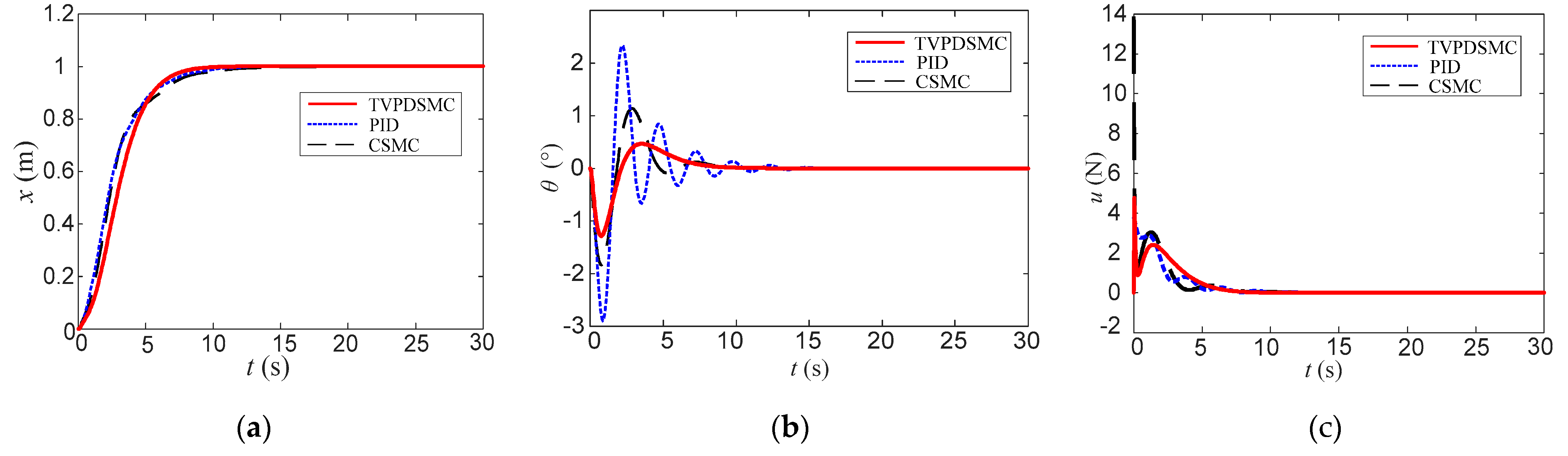
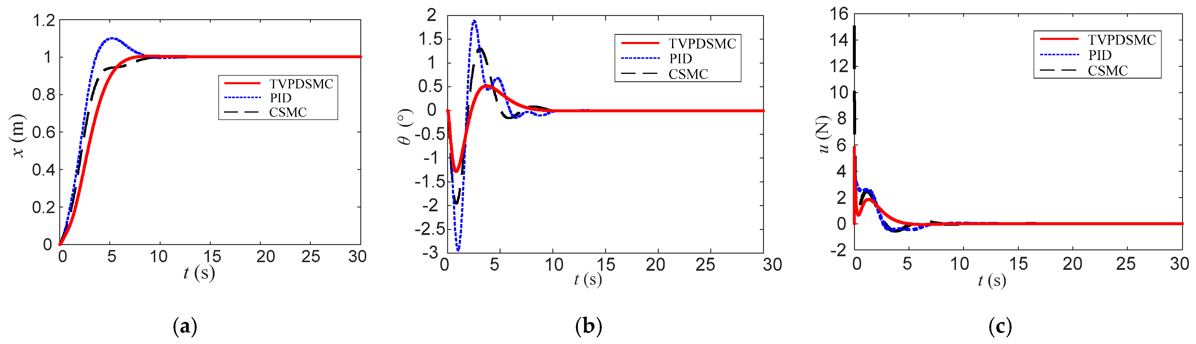
4. Simulation Results and Analysis

In this section, to verify the generality of the application of the proposed controller and its robustness to parameter variations/external disturbances, four sets of rigorous simulations are performed using MATLAB/Simulink. Simulation 1: By applying the same driving force to the crane system under the same initial swing angle interference, the validity of the model and the swing reduction effect of the radial spring-damper are verified; Simulation 2: In the case of selecting the same crane system parameters, the control performance of PID, conventional sliding mode (CSMC) and TVPDSMC is compared; Simulation 3: The robustness and anti-disturbance ability of TVPD-SMC against external interference were tested; Simulation 4: The control performance and robustness of TVPD-SMC under the condition of system parameter variation were tested.

Among them, the friction parameters are set as f_r = 4.4, ε_x = 0.5, k_rx = −0.5 [32], and the gravity acceleration g = 9.8 m/s². The parameters of container crane system are set in

Table 1. Crane system parameters.

Parameters	Symbol	Value
Trolley Mass	M	5 kg
Hook Mass	m1	0.2 kg
Payload Mass	m2	1 kg
Rope Length	L	1.5 m
Cable Spacing on Trolley	d	0.2 m
Cable Spacing on Hook	w	0.18 m
Rotational Inertia	J	0.8 kg/m2
Hook to payload Spacing	R	0.2 m
Elasticity Factor	k	120
Damping Factor	c	1.75

[9,35].

Simulation 1: Model validity verification. In order to verify the validity of the container crane system model and the swing reduction effect of the radial spring-dampers, the following two initial conditions are set under the same system parameters. (1) Give the payload an initial swing angle of 30° while the trolley remains stationary; (2) add a driving force of 1N to the crane system for 5 s. Compare the difference in swing angle state between the crane designed with the radial spring-damper device and the crane without the radial spring-damper. The equations of the dynamics of the container crane system without radial spring-damper design are as follows:

$$\begin{array}{l}(M+m_1+m_2)\ddot{x}+[m_{1}L\cos \theta +m_2(L\cos \theta -aR\cos a\theta )]\ddot{\theta }-[m_{1}L\sin \theta -\\ m_2(a^{2}R\sin a\theta -L\sin \theta )]{\dot{\theta }}^2=u-f\end{array},$$

(44)

$$\begin{array}{l}(m_1+m_2)[\ddot{x}L\cos \theta +L^2\ddot{\theta }]+m_2[-\ddot{x}aR\cos a\theta +a^2{R}^2\ddot{\theta }+(aRL+a^{2}RL)\sin (\theta +\\ a\theta ){\dot{\theta }}^2-2RLa\cos (\theta +a\theta )\ddot{\theta }]+(m_1+m_2)gL\sin \theta +m_{2}gRa\sin a\theta +J{a}^2\ddot{\theta }=0\end{array}.$$

(45)

The results of the simulation experiments are shown in Figure 3. As can be seen from Figure 3a, the amplitude of the crane swing designed with the radial spring-damped device starts to decrease significantly after one cycle under the same initial swing angle disturbance. It can be seen that the nonlinear Coriolis damping provided by the radial spring-damper for the system can effectively dissipate the energy of the payload swing and reduce the payload swing. As can be seen from Figure 3b, under the same driving force, the maximum swing angle of the crane system without radial spring-dampers is 1°, and the maximum swing angle of the container crane with radial spring-dampers is 0.8°, and the steady state is reached more quickly. Therefore, the radial spring-damper has significant damping effect under driving force and can effectively eliminate residual swing.

Simulation 2: Controller comparison experiment. The control performance of the proposed control method is compared with PID and CSMC [29] methods in the same simulation environment. The PID and CSMC control laws are as follows.

(1)

PID control law:

$$F=k_{px}{e}_x+k_{ix}{\displaystyle \int e_x}+k_{dx}{\dot{e}}_x+k_{p\theta }{e}_{\theta }+k_{i\theta }{\displaystyle \int e_{\theta }}+k_{d\theta }{\dot{e}}_{\theta }.$$

(2)

CSMC control law:

$$\begin{array}{l}F=(M+m_1+m_2)(-\alpha \dot{x}+\beta \dot{\theta })+(m_1\sin \theta +m_2\sin \theta )\ddot{r}\\ +[m_1(L\cos \theta +r\cos \theta +m_2(L\cos \theta +r\cos \theta -aR\cos a\theta )]\ddot{\theta }\\ +[-m_1(L\sin \theta +r\sin \theta )+m_2(a^{2}R\sin a\theta -L\sin \theta -r\sin \theta )]{\dot{\theta }}^2\\ +2(m_1+m_2)\cos \theta \dot{\theta }\dot{r}+f-ks-\epsilon \tanh (s)\\ s=\dot{x}+\alpha (x-x_d)-\beta \theta \end{array}.$$

The parameters of the three controllers are shown in

Table 2. Control Gains.

Control Method	Control Gains
PID	kpx = 3.79, kix = 0.007, kdx = 5.611, kpθ = 1.45, kiθ = 33.76, kdθ = 0.15
CSMC	α = 0.43, β = 5.05, k = 24.36, ε = 8.36
TVPD-SMC	γ = 10.58, μ = 1.07, βx = 0.89, kpx = 0.19, kdx = 17.33, λx = 3.42

, and the simulation results are shown in Figure 4. Figure 4 shows that all three methods can accurately transport the trolley to the predetermined position in about 10s. However, the proposed method performs better than the other two methods in terms of swing suppression. Specifically, the maximum swing amplitude of the TVPD-SMC control method is about 1.28°, which is 0.57° smaller than that of the CSMC control method (1.85°) and 1.77° smaller than that of the PID control method (3.05°). In terms of driving force, the driving force required for the TVPD-SMC control method proposed in this paper is smaller than the remaining two controllers. Therefore, the TVPD-SMC designed in this paper has good control effects in all aspects.

Simulation 3: Robustness verification. To verify the anti-disturbance capability of the proposed TVPD-SMC method against external disturbances, the following three external disturbances were artificially added to the payload swing angle during the simulation:

(1)

Sinusoidal disturbances with a relative amplitude of 15% and a frequency of 3.14 Hz between 11 s and 13 s.

(2)

Pulsed disturbances with a relative amplitude of 15% and a pulse width of 0.2 s between 19 s and 19.2 s.

(3)

Random disturbances with a relative amplitude of 15% between 24 s and 26 s.

The relative amplitude is defined as the percentage share of the pendulum angle disturbance amplitude to the maximum payload pendulum amplitude throughout the process. The control parameters are kept consistent with Table 2, and the simulation results are shown in Figure 5.

It can be seen from Figure 5 that under the conditions of simulation 3, the method proposed in this paper can quickly return to the steady state after the end of the disturbance, the trolley motion curve is smoother, and the positioning performance is almost unaffected, while the residual swing angle of the payload can be quickly eliminated. The results show that the TVPD-SMC method has good control performance and strong robustness to various external disturbances.

Simulation 4:Robustness verification. To verify the effectiveness and robustness of the controller under different system parameters, the payload mass is changed from 1 kg to 2 kg, the rope length is changed from 1.5 m to 2 m, the friction coefficient f_r is changed from 4.4 to 2.4, and other system parameters remain unchanged. Control parameters are kept consistent with Table 2, and the simulation results are shown in Figure 6.

As can be seen from Figure 6, the proposed method still maintains good control performance under the condition of changing the system parameters. Specifically, the arrival speed and accuracy of the cart are almost unaffected compared with Simulation 2, and the performance in terms of payload swing suppression and energy consumption remains good. While the PID method and the CSMC controller under the role of the crane system is more affected by the parameters, the control effect is significantly worse, and the PID control method also appears a significantly overshoot phenomenon. This also shows that the TVPD-SMC method has stronger robustness than the other two compared methods.

Remark 5.

Future work on this method will build a real model platform.

5. Conclusions

To narrow the gap between theory and practice and promote the research of container crane, this paper firstly establishes the equivalent double pendulum model of this crane system by using Lagrange modeling technique. In addition, the Coriolis damping force of the radial spring is used to effectively reduce the container crane payload swing. On this basis, a time-varying PD sliding mode control method is proposed. The controller has a simple structure and strong global robustness, and it returns to the equilibrium point faster than the other two existing methods when subjected to external disturbances. The proposed controller is able to guarantee the asymptotic stability of the ideal equilibrium point by a rigorous demonstration of the Lyapunov technique and the Lasalle invariance theorem. Finally, numerical simulation by MATLAB/Simulink verifies the effectiveness of the proposed method and its robustness to external disturbances. In the future work, this paper will aid in extending the proposed method to the three-dimensional case and building a physical experimental platform for multi-rope container cranes, focusing on the anti-swing positioning performance of the payload during the lifting process.

References

1. Ramli, L.; Mohamed, Z.; Abdullahi, A.M.; Jaafar, H.I.; Lazim, I.M. Control strategies for crane systems: A comprehensive review. Mech. Syst. Signal Process. 2017, 95, 1–23. [Google Scholar] [CrossRef]
2. Khatamianfar, A.; Savkin, A.V. Real-time robust and optimized control of a 3D overhead crane system. Sensors 2019, 19, 3429. [Google Scholar] [CrossRef] [PubMed] [Green Version]
3. Lu, B.; Fang, Y.; Sun, N. Nonlinear control for underactuated multi-rope cranes: Modeling, theoretical design and hardware experiments. Control Eng. Pract. 2018, 76, 123–132. [Google Scholar] [CrossRef]
4. Kim, C.S.; Hong, K.S. Boundary control of container cranes from the perspective of controlling an axially moving string system. Int. J. Control Autom. Syst. 2009, 7, 437–445. [Google Scholar] [CrossRef]
5. Park, H.; Chwa, D.K.; Hong, K.S. A feedback linearization control of container cranes: Varying rope length. Int. J. Control Autom. Syst. 2007, 5, 379–387. [Google Scholar]
6. Xu, W.; Gu, W.; Shen, A.; Chu, J.; Niu, W. Anti-swing control of a new container crane with fuzzy uncertainties compensation. In Proceedings of the 2011 IEEE International Conference on Fuzzy Systems (FUZZ-IEEE 2011), Taipei, Taiwan, China, 27–30 June 2011. [Google Scholar]
7. Lu, B.; Fang, Y.; Sun, N. Adaptive trajectory tracking control for a four-rope crane. In Proceedings of the 2015 IEEE International Conference on Advanced Intelligent Mechatronics (AIM), Busan, Korea (South), 7–11 July 2015. [Google Scholar]
8. Kim, G.; Hong, K. Adaptive Sliding-Mode Control of an Offshore Container Crane with Unknown Disturbances. IEEE/ASME Trans. Mechatron. 2019, 24, 2850–2861. [Google Scholar]
9. Lu, B.; Fang, Y.; Sun, N. Modeling and verification for a four-rope crane. In Proceedings of the 2015 IEEE International Conference on Cyber Technology in Automation, Control, and Intelligent Systems (CYBER), Shenyang, China, 8–12 June 2015. [Google Scholar]
10. Masoud, Z.N.; Nayfeh, A.H. Sway reduction on container cranes using delayed feedback controller. Nonlinear Dyn. 2003, 34, 347–358. [Google Scholar] [CrossRef]
11. Masoud, Z.N.; Daqaq, M.F. A graphical approach to input-shaping control design for container cranes with hoist. IEEE Trans. Control Syst. Technol. 2006, 14, 1070–1077. [Google Scholar] [CrossRef]
12. Lu, B.; Cao, H.; Hao, Y.; Lin, J.; Fang, Y. Online Antiswing Trajectory Planning for a Practical Rubber Tire Container Gantry Crane. IEEE Trans. Ind. Electron. 2021, 69, 6193–6203. [Google Scholar] [CrossRef]
13. Barbosa, F.M.; Löfberg, J. Time-optimal control of cranes subject to container height constraints. arXiv 2022, arXiv:2203.15360. [Google Scholar]
14. Wang, N.; Cao, G.; Yan, L.; Wang, L. Modeling and control for a multi-rope parallel suspension lifting system under spatial distributed tensions and multiple constraints. Symmetry 2018, 10, 412. [Google Scholar] [CrossRef] [Green Version]
15. Hoang, U.T.T.; Le, H.X.; Thai, N.H.; Pham, H.V.; Nguyen, L. Consistency of control performance in 3d overhead cranes under payload mass uncertainty. Electronics 2020, 9, 657. [Google Scholar] [CrossRef] [Green Version]
16. Park, H.C.; Chakir, S.; Kim, Y.B.; Lee, D.H. A Robust Payload Control System Design for Offshore Cranes: Experimental Study. Electronics 2021, 10, 462. [Google Scholar] [CrossRef]
17. Pham, H.V.; Hoang, Q.-D.; Pham, M.V.; Do, D.M.; Phi, N.H.; Hoang, D.; Le, H.X.; Kim, T.D.; Nguyen, L. An Efficient Adaptive Fuzzy Hierarchical Sliding Mode Control Strategy for 6 Degrees of Freedom Overhead Crane. Electronics 2022, 11, 713. [Google Scholar] [CrossRef]
18. Jiang, B.; Liu, D.; Karimi, H.R.; Li, B. RBF Neural Network Sliding Mode Control for Passification of Nonlinear Time-Varying Delay Systems with Application to Offshore Cranes. Sensors 2022, 22, 5253. [Google Scholar] [CrossRef] [PubMed]
19. Li, H.; Hui, Y.B.; Wang, Q.; Wang, H.X.; Wang, L.J. Design of Anti-Swing PID Controller for Bridge Crane Based on PSO and SA Algorithm. Electronics 2022, 11, 3143. [Google Scholar] [CrossRef]
20. Bartolini, G.; Pisano, A.; Usai, E. Second-order sliding-mode control of container cranes. Automatica 2002, 38, 1783–1790. [Google Scholar] [CrossRef]
21. Ngo, Q.H.; Nguyen, N.P.; Nguyen, C.N.; Tran, T.H.; Hong, K.S. Fuzzy sliding mode control of container cranes. Int. J. Control Autom. Syst. 2015, 13, 419–425. [Google Scholar] [CrossRef]
22. Ngo, Q.H.; Nguyen, N.P.; Truong, Q.B.; Kim, G.H. Application of Fuzzy Moving Sliding Surface Approach for Container Cranes. Int. J. Control Autom. Syst. 2021, 19, 1133–1138. [Google Scholar] [CrossRef]
23. Wu, Q.; Wang, X.; Hua, L.; Xia, M. Modeling and nonlinear sliding mode controls of double pendulum cranes considering distributed mass beams, varying roped length and external disturbances. Mech. Syst. Signal Process. 2021, 158, 107756. [Google Scholar] [CrossRef]
24. Bessa, W.M.; Otto, S.; Kreuzer, E.; Seifried, R. An adaptive fuzzy sliding mode controller for uncertain underactuated mechanical systems. J. Vib. Control 2019, 25, 1521–1535. [Google Scholar] [CrossRef]
25. Lu, B.; Fang, Y.; Sun, N. Enhanced-coupling adaptive control for double-pendulum overhead cranes with payload hoisting and lowering. Automatica 2019, 101, 241–251. [Google Scholar] [CrossRef]
26. Zhang, M.; Zhang, Y.; Cheng, X. An Enhanced Coupling PD with Sliding Mode Control Method for Underactuated Double-pendulum Overhead Crane Systems. Int. J. Control Autom. Syst. 2019, 17, 1579–1588. [Google Scholar] [CrossRef]
27. Masoud, Z.; Alhazza, K.; Abu-Nada, E.; Majeed, M. A hybrid command-shaper for double-pendulum overhead cranes. J. Vib. Control 2014, 20, 24–37. [Google Scholar] [CrossRef]
28. Wang, T.; Tan, N.; Zhang, X.; Liu, R.; Qiu, J.; Zhou, J.; Hao, X. An Enhanced Coupling Adaptive Sliding Mode Control Method for Casting Cranes Based on Radial Spring Damping. Math. Probl. Eng. 2022, 2022, 6519175. [Google Scholar] [CrossRef] [PubMed]
29. Tuan, L.A.; Lee, S.G. Sliding mode controls of double-pendulum crane systems. J. Mech. Sci. Technol. 2013, 27, 1863–1873. [Google Scholar] [CrossRef]
30. Sun, N.; Wu, Y.; Fang, Y.; Chen, H.; Lu, B. Nonlinear continuous global stabilization control for underactuated RTAC systems: Design, analysis, and experimentation. IEEE/ASME Trans. Mechatron. 2016, 22, 1104–1115. [Google Scholar] [CrossRef]
31. Ma, B.; Fang, Y.; Liu, X.; Wang, P. Modeling and Simulation Platform Design for 3D Overhead Crane. J. Syst. Simul. 2009, 21, 3798–3803. (In Chinese) [Google Scholar]
32. Zhang, M.; Ma, X.; Song, R.; Rong, X.; Tian, G.; Tian, X.; Li, Y. Adaptive proportional-derivative sliding mode control law with improved transient performance for underactuated overhead crane systems. IEEE/CAA J. Autom. Sin. 2018, 5, 683–690. [Google Scholar] [CrossRef]
33. Chang, T.; Hurmuzlu, Y. Sliding Control Without Reaching Phase and Its Application to Bipedal Locomotion. ASME. J. Dyn. Sys. Meas. Control 1993, 115, 447–455. [Google Scholar] [CrossRef] [Green Version]
34. Bartoszewicz, A.; Nowacka, A. Sliding-mode control of the third-order system subject to velocity, acceleration and input signal constraints. Int. J. Adapt. Control Signal Process. 2007, 21, 779–794. [Google Scholar] [CrossRef]
35. Duc, V.L.; Youngjin, P. A Cable-Passive Damper System for Sway and Skew Motion Control of a Crane Spreader. Shock Vib. 2015, 2015, 507549. [Google Scholar]
Figure 1. Two-dimensional model of crane system.
Electronics 11 03543 g001
Figure 2. Equivalent double pendulum model.
Electronics 11 03543 g002
Figure 3. Simulation 1: Pendulum angle response curve. (a) Pendulum angle response curve under the same initial pendulum angle disturbance; (b) Pendulum angle response curve under the same driving force.
Electronics 11 03543 g003
Figure 4. Simulation 2: System state variable response curve. (a) Trolley Displacement; (b) Payload Swing angle; (c) Driving force.
Electronics 11 03543 g004
Figure 5. Simulation 3: System state variable response curve. (a) Trolley Displacement; (b) Payload Swing angle; (c) Driving force.
Electronics 11 03543 g005
Figure 6. Simulation 4: System state variable response curve. (a) Trolley Displacement; (b) Payload Swing angle; (c) Driving force.
Electronics 11 03543 g006