Abstract
Acoustic signal classification plays a central role in acoustic source identification. In practical applications, however, varieties of training data are typically inadequate, which leads to a low sample complexity. Applying classical deep learning methods to identify acoustic signals involves a large number of parameters in the classification model, which calls for great sample complexity. Therefore, low sample complexity modeling is one of the most important issues related to the performance of the acoustic signal classification. In this study, the authors propose a novel data fusion model named MFF-ResNet, in which manual design features and deep representation of log-Mel spectrogram features are fused with bi-level attention. The proposed approach involves an amount of prior human knowledge as implicit regularization, thus leading to an interpretable and low sample complexity model of the acoustic signal classification. The experimental results suggested that MFF-ResNet is capable of accurate acoustic signal classification with fewer training samples.
1. Introduction
Acoustic signal classification plays a central role in acoustic source identification [1], including many applications, such as marine animal [2], civil aviation aircraft [3], and noise source identification [4,5]. Generally, this problem can be solved in two different ways, the first one is to classify acoustic signals with manual design features, the model of which is low expressive but easy to interpret. The other is learning with deep representation features, the model of which is high expressiveness but calls for a huge amount of sample complexity. This manuscript provides a novel features fusion model with bi-level attention mechanism, which has a feature enhancement module and a feature fusion module. This approach involves an amount of prior human knowledge as implicit regularization, thus leading to an interpretable and low sample complexity model of the acoustic signal classification.
Classic sound signal identification methods include GMMs (Gaussian mixture models), SVMs (support vector machines), HMMs (hidden Markov models), and other classic machine learning methods [6]. They include manual identification and are therefore able to generate accurate results. Stephen So et al. have worked on sound classifiers based on Gaussian mixture models (GMMs) and leverage MFCC to improve the identification performance of the algorithms [7]. Bittle and Duncan et al. incorporate the support vector machine (SVM) sound target classification technology in sound source identification and classify the signal based on the similarity between the unknown signal and the model training data [8]. Further, Daniele Salvati et al. propose a support vector machine (SVM) with a kernel function of RBF and construct a weighted MVDR beamformer, which works well in near-field single sound source identification. However, the array gain of the conventional beamformer is limited. In order to maximize the array gain, Capon proposed the MVDR beamformer in 1969 [9,10]. Walters et al. propose applying the random forest method to acoustic classification so as to achieve training on large-scale datasets [11]. Zilli Parson et al. apply the hidden Markov model (HMM) to acoustic analysis and classification because this model is able to fuse the sound signal and the temporal details in the sequence [12]. The methods described above, however, because of their incapability of automatic feature extraction, typically perform poorly when recognizing new signals; they are still needful of a new algorithm. This restricts their scope of application and diminishes their generalization ability.
In recent decades, deep learning [13] has provided state of the art performance in lots of areas including text [14], images [15], and sound data analysis [16], because it can solve problems in a big range of complex pattern recognition. It has equally given excellent results in the classification of acoustic signals. Pirotta et al. explore applying unsupervised learning to acoustic signal classification and make grouping based on the similarity of features between data (cluster algorithm) [17]. Goeau and Mac Aodha have studied the convolutional neural network technology without feature pre-processing and propose identifying features directly from the spectrogram data, which avoid the noise-sensitive feature extraction stage [18]. Boqing Zhu et al. propose a CNN architecture, where the network is integrated for multi-time resolution analysis and multi-level feature extraction, which solves the multi-scale problem in environmental acoustic classification [19]. Oikarinen et al. introduce a convolutional neural feedforward network, where the original spectrogram is taken as input, enabling classifying the source and type of acoustic signals in a noisy environment [20]. However, in real applications, it is expensive or even impossible to gain varieties of samples, such as medical imaging and 3D reconstruction. In addition, these traditional deep neural networks do not involve manual domain knowledge, which is prone to overfitting and poor interpretability even under heavy data augmentations.
Therefore, researchers are interested in improving deep learning models and with fewer training samples. A straightforward idea is data enhancement techniques [21]. Several training data generators have been proposed, such as deep learning under conditions of Gaussian noise [22,23] or object attributes [24]. Nonetheless, when being trained on small sample data, such data generators often fare poorly [25]. The second solution is to optimize the neural network algorithm. Erhan et al. investigate unsupervised pre-training in deep learning and substantiate the generalization effect of pre-trained network weights experimentally [26]. Yu-Xiong Wang et al. suggest a method that works, by means of unsupervised data sources to improve the overall transferability of supervised CNNs, thereby permitting the identification of new classes from a small number of samples [27]. Mishkin and Matas propose the initialization of variances of layer sequence units, whereby the weight of each convolutional layer is initialized through an orthogonal matrix so that the weights are normalized into unit variance [28]. The third method is to adjust the structure of the neural network model. Qianru Sun et al. propose a meta-transfer learning (MTL) method, which is able to transfer the weights of a deep neural network with fewer training samples [29]. Mengye Ren et al. proposes a semi-supervised small sample size learning mode to learn how to make use of unlabeled samples, which improve model performance under semi-supervision [30]. Mark Woodward proposes an active learning method that combines reinforced learning with small sample-size learning to achieve higher prediction accuracy than pure supervised models [31].
The overall goal of this manuscript is to identify the acoustic source with low sample complexity, which intends to overcome the bottleneck of the current deep learning methodology. In this study, a novel bi-level attention mechanism was proposed to fuse the handcraft features and deep representation features in order to include more prior human knowledge, thus a low sample complexity to train the neural network. The main contributions of this paper are the construction of two sub-networks, named feature enhance module and feature fusion module, respectively. In the feature enhance module, this study applies scaled dot-product attention to local level enhancing of both handcraft features and deep representation features. In the feature fusion module, the manuscript modifies the self-attention to obtain a global fusion of the enhanced features.
To verify the model we proposed, this study was tested on a public dataset named Esc: Dataset for environmental sound classification [32], and another dataset was collected by this research. This study chose four different models for comparison, such as the classical rResNet, the state of art method EnvNet [33], EnvNet v [34], GoogLeNet [35], MFF-ResNet (without bi-level attention), and MFF-ResNet (without rResNet) for ablation experiment. The experiment suggested that the MFF-ResNet performs quite well on a small sample training set of sound source classification compared with baseline methods.
This paper is so structured that in Section 2, the current deep learning methods for processing spectrograms are discussed. Section 3 presents the MFF-ResNet model and describes its structure. Section 4 describes the experiment and gives an analysis of the experimental results. Section 5 provides a summary of this paper.
2. Background
2.1. Data Pre-Processing
As shown in Figure 1, the sound data are collected by the acoustic signal acquisition equipment with different channels of . The original signals are waveforms represented in the time domain. To analyze the power spectrum properties, it is necessary to convert the original signals with certain integral transform, such as Fourier transform or wavelet transform. Due to the power, spectrum contains the characteristic information of the source signal in different frequency bands at different times, similar as image processing, and a deep convolutional network can be applied in high-level feature representation.
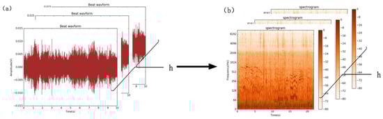
Figure 1.
The form of sound data for channels. When sound is converted into tensor data, for each channel, data is represented as (time_steps, features) two-dimensional time series information, as shown in (a). The spectrogram contains the sound’s time-frequency domain information, as shown in (b).
In the field of sound signal processing, MFCC (Mel frequency cepstrum coefficient) is often extracted during audio analysis, but this causes a big loss of sound details. After the birth of deep learning, thanks to the powerful feature extraction capability of deep neural networks, it becomes possible to allow the neural network to extract more robust features by feeding the log-Mel spectrum (or power spectrum) information directly into the neural network for training, as shown in Figure 2.
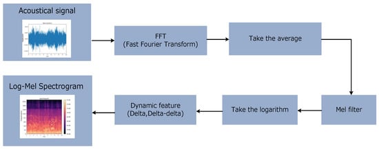
Figure 2.
The acquisition of log-Mel spectrogram. After a series of operations, such as the fast Fourier transform, taking the average, Mel filter, logarithm, and extraction of dynamic features, the log-Mel spectrogram features of the acoustic signal data are obtained as the form of (frequency, time_steps, channel).
2.2. Related Works
The diagrammatic sketch in Figure 3 depicts the general procedure for acoustic signal classification. Firstly, a microphone array consisting of high-sensitivity omnidirectional sound sensors collected sound signals from different sound sources. After data pre-processing, manual design features and log-Mel spectrogram were extracted to obtain the manual design classification features in the form of number of manual features, number of frames, or number of channels and the log-Mel spectrogram features in the form of (frequency, time_steps, channel). Secondly, a deep learning training network suitable for acoustic signal data was constructed, such as ResNet. Finally, the network model was trained and then tested for its performance through experiments.
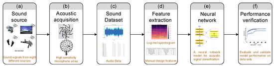
Figure 3.
Diagrammatic of acoustic signal classification: Panels (a–c) are for sound signal acquisition and storage. Sound signals from different sound sources are collected through the microphone array and stored as audio data. (c) The LSE (low-sample environmental) dataset is collected by hardware equipment of sound signal acquisition. The original signals in LSE dataset are waveforms represented in the time domain. The sound signal achieved by the signal hardware acquisition device is converted into an electrical signal and processed. Thus, the sound source signals are changed with time. As shown in panel (d), after feature extraction, a log-Mel spectrogram and a series of manual design features are obtained. In panel (e), a neural network is used to classify acoustic signals. Finally, we tested the model for its performance, as showed in panel (f).
It is apparent that the main issue in acoustic signal classification is designing a neural network to learn, represent, and fuse data features. Due to the strong expressive ability of neural network, deep learning models have achieved extraordinary performance compared with traditional signals’ processing methods. However, experiments showed that after the network has reached a certain depth, a further greater number of layers do not lead to further improvement in classification performance but rather leads to slower network convergence and worse classification accuracy. One of the most widely used approaches is named ResNet [36], which was proposed to resolve this problem based on the concept of residual representation. The schematic diagram of the residual block and a typical ResNet is shown in Figure 4a.
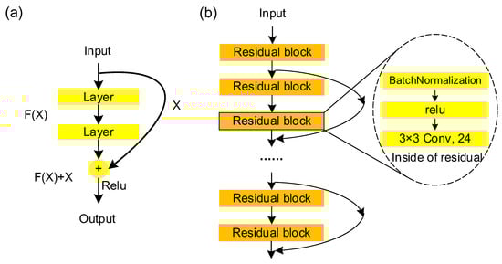
Figure 4.
The residual block (a) and the residual network (b). Here is any two-dimensional input signal. represents the transform by the residual block.
The signals put in ResNet can be directly connected to an earlier layer through a shortcut, so that a large number of effective features are still retained at the end of the network, and the feature signals in the data are fully exploited, which can maintain a strong increase momentum in accuracy with an increasing depth as shown in Figure 4b. This makes the ResNet classification network the most widely used CNN feature extraction network.
Recently, Anam Bansal uses a deep neural network method to verify its superiority in ambient sound classification performance [37]. Ref [38] proposed an attention-based ResNet, which used attention-guided deep model to efficiently learn spatial-temporal relationships that exist in the spectrogram of a signal. In this study, we aim to train ResNet with low sample complexity, thus using bi-level attention mechanisms to enhance and fuse deep representation features with the handcraft features, in order to include more prior knowledge.
3. Methodology
3.1. The Architecture of MFF-ResNet
To classify acoustic signals with low sample complexity, this study proposes a novel bi-level attention mechanism to fuse the handcraft features and deep representation features in order to include more prior human knowledge, thus a low sample complexity to train the neural network. As depicted in Figure 5, the log-Mel spectrogram features and manual design features fusion ResNet (MFF-ResNet) are proposed.
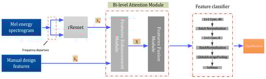
Figure 5.
MFF-ResNet. The inputs of MFF-ResNet are log-Mel spectrogram features and manual design features. The two branch outputs of the spectrogram features were used for frequency fusion with rResNet (as shown in Figure 6). The more abstract features are obtained by the bi-level attention module, which includes a features enhancement and a fusion module (as shown in Figure 7 and Figure 8, respectively). The fused features are then passed through the feature classifier to produce the final classification results.
As the input of the proposed network, log-Mel spectrogram features and manual design features are included in this fusion model. Then, the deep represented Mel spectrogram is pertained with fine-tuned rResNet. Sequentially, deep represented features and manual design features are fused with a bi-level attention module. Finally, a feature classify module is applied for the downstream task.
3.2. Manual Design Features
Manual design features are based on the feature engineering method [39]. Manual design is completed beforehand and features are extracted from audio signals. Manual design features are most concerned with the overall recognition of acoustic signals, such as pitch, tone, and silence rate. By means of manual design features, meaningful data features are derived from the data. High-quality features help to improve the overall performance and accuracy of this model. Features basically concern basic problems, and it is necessary to design features related to scenes, problems, and domains.
The open-source audio analysis software Essentia [40], more specifically, it’s feature extractor Freesound, was used to extract manual features from the acoustic data. First, the audio file was framed such that a 10-s sound signal was divided into 500 frames, each frame signal being 40 ms, with 20 ms of overlap between adjacent frames.
Feature extraction was performed with Freesound: For each frame signal in a single channel, the Freedsound’s feature [41] extraction function (parameters were set to the default values) was used to extract 400 features, as shown in the Table 1. From each sound sample, Freesound manual design acoustic source features were extracted in the form of (number of manual features, number of frames, number of channels).

Table 1.
The features picked up by the Freesound feature extractor.
3.3. Deep Representation Features with Fine-Tuned rResNet
3.3.1. rResNet
The log-Mel spectrogram data in the form of (frequency, time_steps, channel) were split along the frequency axis into the first half low-frequency band and the second half high-frequency band. Because of that, the high-frequency and low-frequency parts of the data had different forms of characteristics. Inspired by wavelet nets, the ResNet in the frequency framework of this study is improved. The frequency energy is separated into a high-frequency part and a low-frequency part. The convolution can be the type of filter that is desired; this study used skip connection only for the high-frequency part, and then this modified ResNet was named as rResNet, which is shown in Figure 6.
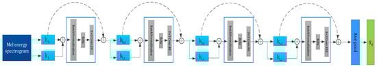
Figure 6.
r-ResNet. The input of rResNet is the Mel energy spectrogram. Sequentially, this paper decomposes the frequency into high-frequency part and low-frequency part , respectively. The classical ResNet is modified by only adding a skip connection branch of high-frequency part . This study justifies this because convolution is a low pass filter, if high-frequency part passes the low pass filter that will lose a lot of detail information.
The convolution kernel size of these convolutions in the network was 3 × 3; the padding was set to “same” so that each time the data passed through the convolution layer only its channel number was changed, but the frequency axis and the dimensions of the time axis were preserved. For the sake of subsequent frequency axis dimension fusion, no down-sampling was performed. After the pre-trained network, the outputs from the two paths were fused by concatenation operations on the frequency axis, to revert to the frequency dimension of the original data, which completed the frequency fusion.
3.3.2. Pre-Training and Fine-Tuning Technology
A common and very efficient way to apply deep learning to small sample datasets is to use a pre-trained network [42,43,44,45,46]. A pre-trained network is a model that has already been trained on a large dataset. If the original dataset is large and general enough, the feature space hierarchy learned by the pre-trained network can work effectively as a general model for acoustic analysis. Therefore, these features can help solve various acoustic signal classification problems, even if these new problems involve classes that are completely different from the original task.
In this section, this manuscript represents a pre-training and fine-tuning technology for the backbone network named rResNet. Pre-training and fine-tuning technology was widely used in the acoustic scene and event detection classification task, such as DCASE. As shown in Figure 9, the approach of this study first keeps the convolution part only of the network for feature extraction, so that the classifier part of the pre-trained network was discarded but uses a new classifier adapted to this training data. Inspired by the fact that the generality (and reusability) of feature extraction of a convolutional layer depends on the depth of the layer in the model. The deeper the layer in the model, the more abstract the extracted concept is. Since the new dataset differed much from the dataset used to train the original model, only the beginning part of the model was used for feature extraction with the deeper layers being trained along with the newly included classifier. Thus, this study next freezes the low-level convolutional to fine-tune high-level convolutional. The convolution part of the pre-trained network ResNet contained 12 convolutional layers, the first 8 of which were of frozen weights. The weights of the rest 4 convolutional layers were unfrozen. By training the weights of these deeper convolutional layers, the abstract representation of the model was made more relevant to the classification problem in question.
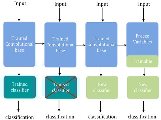
Figure 9.
Fine-tuned ResNet. Firstly, the classifier of the pre-trained network was substituted by a feature classifier, which was adapted to this training data. Secondly, the model weights in the low-level convolution part were frozen. It was justified because the previous part of the convolution was used for feature extraction, and the deeper convolutional layer with a more abstract concept was trained along with the feature classifier. Finally, we fine-tuned a high-level convolution part according to training data.
3.4. Feature Fusion Based on Bi-Level Attention
In order to encode prior human knowledge as implicit regularization, this study develops a robust and an efficient features fusion strategy based on bi-level attention. The motivation lies on the manual design features providing an abundant interpretation and deep representation of features providing an expressive abstraction of the given acoustic signal. Thus, fused features contain much useful prior information and a good description of the acoustic signal features.
The features fusion strategy of this study consists of two modules, named features enhancement module and feature fusion module, respectively. Both of these modules are constructed based on the attention mechanism. Inspired by the selective visual mechanism of humans, the attention mechanism can filter out the most influential parts from a large amount of information according to certain queries.
3.4.1. Features Enhancement Module
Without loss of generality, suppose manual designed features are denoted as , in the form of (features, time-steps, channel) and the deep representation features are denoted as . As shown in Figure 7, in order to enhance deep representation features , the Features Enhancement Module firstly applies convolution to adjust the input channel numbers and then uses an interpolation method (resampling) to adjust the dimension, thus leading to modified manual design features as . This paper use as quires to reweight deep representation features into , in order to give greater weight to important components and give less weight to unimportant components. The weights of the components are obtained by the softmax function of the inner product between and. The mathematical expression is:
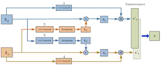
Figure 7.
Features Enhancement Module. Deep representation features and manual designed features are enhanced by scaled dot-product attention. The convolutions at positions 2 and 3 are used to extract the feature parameters of Xd and Xh, and the convolutions at positions 1 and 4 are used to match the number of feature channels extracted. Resampling operation applies the interpolation method to adjust the features’ dimensions in order to operate dot-product.
It was noted here that there are no additional parameters involved in this module. Similarly, this study can enhance manual design features into .
3.4.2. Features Fusion Module
In the Feature Fusion Module as shown in Figure 8, this study slightly modifies the multi-head attention in order to fuse the enhanced manual design and deep representation features . Instead of computing attention only once, the multi-head mechanism runs multiple scaled dot-product attention (SDPA) in parallel. However, the original SDPA requires the same length of input for computation. Thus, this study first concatenates and into a feature vector For each channel , this paper uses a Matlab-like notation as . Sequentially, “Softmax” functions are applied to compute each as follows
with , , and as all learnable parameters.
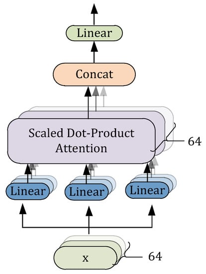
Figure 8.
Features fusion module. Deep representation features and manual designed features are fused with multi-head attention. This study duplicates the input signal and, respectively, puts them into three branches to construct key, query, and value. For each channel of , linear transforms are used to compute each attention head. Finally, the independent attention outputs are simply concatenated and linearly transformed to the expected dimension.
Finally, the independent attention outputs are simply concatenated and linearly transformed to the expected dimension, thus the multi-head attention can be described as:
Here, are also learnable parameters.
3.5. Feature Classifier Module
After being processed by the Feature Fusion Module, the fusion feature was input into the feature classifier. The feature classifier was comprised of two convolutional layers with a kernel size of 1 × 1 and subsequent additional layers. The number of convolution kernels of the first layer was 48, and the number corresponding to the second layer was reduced to the number of classes. What followed were the batch normalization layer, the global average pooling layer, and softmax. The two 1 × 1 convolution layers acted as a two-layer fully connected neural network. Finally, the softmax activation layer assigned weights to the contribution of each channel to arrive at the probability of the sample in each class.
4. Experiment and Result Analysis
4.1. Acoustic Dataset Collection (LSE)
In the experiment to verify the proposed model, this paper built a spherical acoustic sensor array of MicW i436 omnidirectional recording microphones. An acoustic signal hardware acquisition system was created using the hardware acquisition circuit module at the back end to collect multiple sound source signals, as shown in Figure 8. This study collected acoustic signal data from eight different sound source scenes, each source containing 1000 samples to a total of 8000 sample datasets. Each sample lasted 10 s, as shown in Figure 10a–d.
The detailed acquisition process is as follows,
- (a)
- Data acquisition: Firstly, this study connected the source of the excitation device with an external instrument (such as a laptop). Secondly, this study controlled the two kinds of sound source excitation devices to generate sound signal and noise, respectively, in order to guarantee the signal-to-noise ratio of less than −10 dB. It can be noted here, the source signals of sound include eight categories, such as airplane, bus, footstep, car, piano, gun, dog, and vocals. Each kind of sound source signal is a prepared audio file. The Gaussian white noises are immerged into sound signals according to certain signal-to-noise ratio setting. Finally, this study controls the microphone array to collect multi-channel acoustic signals and transmit them to the storage device.
- (b)
- Data slicing: After the data acquisition, the acoustic signal is sliced and processed into multiple eight-channel audio short signals with duration of 10 s.
- (c)
- Data preparation: After slicing the collected data, this study stores each kind of sound source into an intendent file, respectively. For each kind of sound sources, 2000 samples were collected. Therefore, there are totally 16,000 sound signal samples in the LSE (low-sample environmental) dataset. The proportion of the training set, validation set, and test were allocated as 6:2:2. The acoustic classification network model is learned and trained on the training dataset of this dataset.

Figure 10.
Acquisition of acoustic signals: (a–c) are directional speakers, rigid ball microphone array, and acoustic signal acquisition equipment. (d) is the collected 10 s acoustic signal expressed in python.
Figure 10.
Acquisition of acoustic signals: (a–c) are directional speakers, rigid ball microphone array, and acoustic signal acquisition equipment. (d) is the collected 10 s acoustic signal expressed in python.

4.2. Experiment
4.2.1. Ablation Experiment Based on LSE Dataset
Manual design feature extraction and log-Mel spectrogram extraction were performed on the dataset. First, this study performs log-Mel spectrogram extraction on the audio signal, as shown in Figure 11, and manual design feature extraction. In this experiment, a window size of 2048, hop length of 1024 was chosen and 128 n-mels, using the librosa implementation. The resulting spectrograms consisted of 469 time samples and 128 frequency bins. This study calculated the log-Mel deltas and delta-deltas without padding, which reduced the number of time samples to 461. Additionally, the labels (eight folds) were converted into one hot vector using one-hot-encode method.
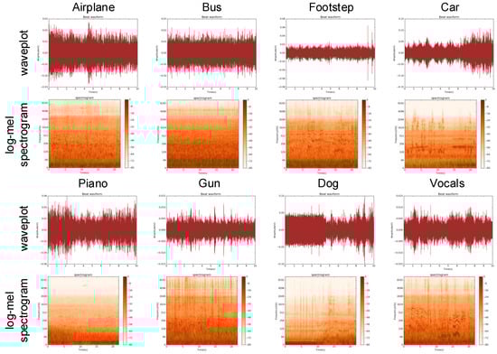
Figure 11.
Wave plot and log-scaled Mel-spectrogram of eight different sound source scenes. It can be clearly seen that there are obvious differences between the sound fragments of different types of sound sources.
These features were then loaded into MFF-ResNet for training. Stochastic gradient descent was included in the training. The amount of batch processing was 32, the loss function was binary-cross entropy, the optimizer was SGD, and the number of epochs was set to 500. The learning rate reset scheduling method was used so that, after completing 3, 8, 18, 38, 128, and 256 iterations, the learning rate was reset to the maximum value of 0.1. After that, the rate attenuated to 0.00001 in accordance with the cosine function. To compare the network performance, the pre-trained network rResNet was used to complete a training of 500 iterations on log-Mel spectrogram features.
To verify the generalization ability of the proposed model, in this study, K-folds cross-validation technique is used to analyze the average experimental results on the test dataset. Specifically, the dataset is divided into K parts. Each subset is disjointed, and the size is the same. One part is selected from the K parts as the verification set, and the remaining K-1 parts are used as the training set. In this way, K separate model training and verification are carried out. Finally, the K verification results are averaged as the verification error of this model. It can be noted here, the K of this study is chosen at 10.
Table 2 shows the ablation result based on MFF-ResNet model and the rResNet (without bi-level attention) based on the collected LSE dataset. Six measures including loss, precision, recall, final accuracy, and epochs of model fitting are used to evaluate the model performance. The result shows bi-level attention can improve the rResNet a lot in general.
Table 2.
Performance comparison under low sample complexity based on the LSE dataset.
Figure 12 shows the classification accuracy and loss corresponding to MFF-ResNet and rResNet. It can be seen that with MFF-ResNet, the classification accuracy stabilizes at 90.15% in the end, and the loss value is as low as 0.34; the classification accuracy of rResNet reaches 76.28%, and the loss value is as low as 0.60. With MFF-ResNet, convergence happens after 160 iterations, which is faster than rResNet’s 210 iterations; and MFF-ResNet is capable of classification accuracy, as shown in Table 2. It can be seen that MFF-ResNet can complete an effective and accurate classification and recognition of the sound characteristics of different sound source targets.
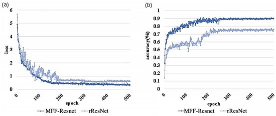
Figure 12.
Performance comparison between MFF-ResNet model and pre-trained rResNet: Panels (a,b) show the changes in loss and accuracy with the number of epochs in network training.
To examine the performance under different training data sizes, this study created a data subset of 1000, 1500, …, 4500, 5000, …, 7500, and 8000 training samples out of the 8000 sample datasets. The accuracy of different models trained on different sample sizes, as revealed by training samples of different data subsets in the comparative experiment, is shown in Figure 13.
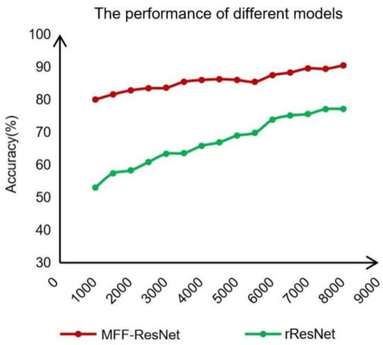
Figure 13.
Contrast experiment with different numbers of training samples.
Figure 13 depicts the change in classification accuracy finally achieved by each model trained on different training sample sizes. The results show that, compared with rResNet, MFF-ResNet performs better in each data subset and shows better recognition performance in small sample data subsets, such as 1000, 2000, 3000, and 4000 samples. Additionally, when manual design features, pre-trained network rResNet, and bi-level attention were used, the model achieved high recognition accuracy with a small number of training samples. The incorporation of manual design features, the contribution of pre-trained network rResNet, and the bi-level attention have so increased the features available to the model that even on a small number of training samples for MFF-ResNet was still able to achieve a good recognition accuracy.
4.2.2. Comparison with the State of Art Methods Based on ESC10
In this section, this study is going to evaluate the performance of MFF-ResNet based on an open data set named ESC-10. ESC-10 is a labeled set of 400 environmental recordings (10 classes, 40 clips per class, 5 s per clip). It is a subset of the larger ESC-50 dataset.
Compared methods include EnvNet, EnvNet2, and GoogLeNet. The results for each method are evaluated using four indicators, such as precision, recall, F1-score, and accuracy. Average test results also used the K-fold cross-validation technique. Table 3 demonstrated that the method proposed in this paper exhibits obvious advantages on average.
Table 3.
Comparison of algorithms based on ESC10 datasets (the best performance is underlined).
The confusion matrix of experimental results on the ESC10 dataset is shown in Figure 14. It can be seen that the network is more sensitive to instantaneous sharp sound signals, so it is more accurate in recognizing dog bark and baby cry, and it is more accurate for sound signals widely distributed on the time domain axis. Less sensitive sound energies, such as rain and rooster, are mostly concentrated in the low-frequency end, making it difficult for the network to accurately identify.
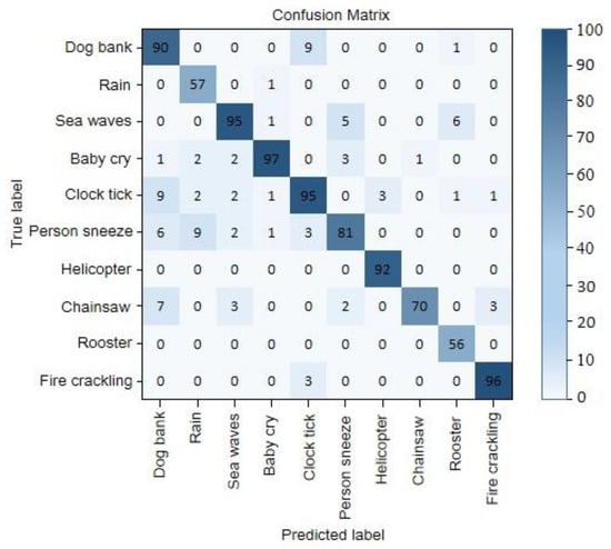
Figure 14.
Confusion matrix for three datasets in ESC-10.
5. Discussion and Conclusions
In sound source recognition and detection applications, data-driven convolutional neural network training with low sample complexity is a key requirement for deep learning in sound signal classification. Because in the field of sound source recognition, data collection is a costly process, which leads to a lack of large-scale sample sets. To alleviate such embarrassment, this paper proposes to fuse spectrogram features and manual design features with a novel attention-based model named MFF-ResNet. It seems bi-level attention can achieve both local enhancement and global fusion of the input signals.
The proposed classification model is flexible, able to handle training tasks based on both large and small databases. As part of future work, this algorithm can also be extended to other application fields, such as medical image recognition, face recognition and face camouflage, face matching and video, and face sketching and photo matching.
Author Contributions
The idea and design of the method were proposed by M.C. and Y.L.; the theoretical analysis of the method was performed by Y.L., P.W. and Y.W.; the experiment was completed at Y.L. and M.C. All authors participated in the revision of the manuscript. All authors have read and agreed to the published version of the manuscript.
Funding
This work was supported by the National Science Foundation of China (No.61901419), Shanxi Provincial Youth Fund Funding (No.201801D221205), Shanxi Provincial University Innovation Project Funding (No.201802083), “13th Five-Year” Equipment Pre-research Weapons Industry Joint Fund (No. 6141B012895),Equipment Pre-research Weapon Equipment Joint Fund (No.6141B021301), Shanxi Provincial Natural Fund Project (No. 201901D111158), National Defense Key Laboratory of Electronic Testing Technology of China Under Project (No.6142001180410), Fundamental Research Program of Shanxi Province (No.20210302123025), Fast Support Programs Weapon Equipment (NO.JZX7Y20220141200501), Scientific and Technological Innovation Programs of Higher Education Institutions in Shanxi, China (No. 2019L0580) and the Joint Funds of the Natural Science Foundation of China (No.U21A20524).
Data Availability Statement
Not applicable.
Conflicts of Interest
The authors declare there is no conflict of interest regarding the publication of this paper.
References
- Isnard, V.; Chastres, V.; Viaud-Delmon, I.; Suied, C. The time course of auditory recognition measured with rapid sequences of short natural sounds. Sci. Rep. 2019, 9, 8005. [Google Scholar] [CrossRef] [PubMed]
- Ruben Gonzalez-Hernandez, F.; Pastor Sanchez-Fernandez, L.; Suarez-Guerra, S.; Alejandro Sanchez-Perez, L. Marine mammal sound classification based on a parallel recognition model and octave analysis. Appl. Acoust. 2017, 119, 17–28. [Google Scholar] [CrossRef]
- Sanchez Fernandez, L.P.; Sanchez Perez, L.A.; Carbajal Hernandez, J.J.; Rojo Ruiz, A. Aircraft Classification and Acoustic Impact Estimation Based on Real-Time Take-off Noise Measurements. Neural Processing Lett. 2013, 38, 239–259. [Google Scholar] [CrossRef]
- Zhang, L.Y.; Ding, D.D.; Yang, D.S.; Shi, S.G.; Zhu, Z.R. Noise source identification by using near field acoustic holograpy and focused beamforming based on spherical microphone array with random unifrom distribution of elements. Acta Phys. Sin. 2017, 66, 12. [Google Scholar] [CrossRef]
- Li, J.; Guo, J.; Sun, X.; Li, C.; Meng, L. A Fast Identification Method of Gunshot Types Based on Knowledge Distillation. Appl. Sci. 2022, 12, 5526. [Google Scholar] [CrossRef]
- Qiu, L. Non-linguistic Vocalization Recognition Based on Convolutional, Long Short-Term Memory, Deep Neural Networks; University of California: Los Angeles, VA, USA, 2018. [Google Scholar]
- So, S.; Paliwal, K.K. Scalable distributed speech recognition using Gaussian mixture model-based block quantisation. Speech Commun. 2006, 48, 746–758. [Google Scholar] [CrossRef]
- Bittle, M.; Duncan, A. A review of current marine mammal detection and classification algorithms for use in automated passive acoustic monitoring. In Proceedings of the Annual Conference of the Australian Acoustical Society 2013, Acoustics 2013: Science, Technology and Amenity, Victor Harbor, Australia, 17–20 November 2013; pp. 208–215. [Google Scholar]
- Salvati, D.; Canazza, S. Adaptive Time Delay Estimation Using Filter Length Constraints for Source Localization in Reverberant Acoustic Environments. IEEE Signal Processing Lett. 2013, 20, 507–510. [Google Scholar] [CrossRef]
- Capon, J. High-resolution frequency-wavenumber spectrum analysis. Proc. IEEE 1969, 57, 1408–1418. [Google Scholar] [CrossRef]
- Walters, C.L.; Freeman, R.; Collen, A.; Dietz, C.; Fenton, M.B.; Jones, G.; Obrist, M.K.; Puechmaille, S.J.; Sattler, T.; Siemers, B.M. A continental-scale tool for acoustic identification of European bats. J. Appl. Ecol. 2012, 49, 1064–1074. [Google Scholar] [CrossRef]
- Zilli, D.; Parson, O.; Merrett, G.V.; Rogers, A. A hidden Markov model-based acoustic cicada detector for crowdsourced smartphone biodiversity monitoring. In Proceedings of the Twenty-Third International Joint Conference on Artificial Intelligence, Beijing, China, 3–9 August 2013; pp. 2945–2951. [Google Scholar]
- LeCun, Y.; Bengio, Y.; Hinton, G. Deep learning. Nature 2015, 521, 436–444. [Google Scholar] [CrossRef]
- Jaderberg, M.; Simonyan, K.; Vedaldi, A.; Zisserman, A. Reading Text in the Wild with Convolutional Neural Networks. IJCV 2016, 116, 1–20. [Google Scholar] [CrossRef]
- Lakhani, P.; Gray, D.L.; Pett, C.R.; Nagy, P.; Shih, G. Hello World Deep Learning in Medical Imaging. J. Digit. Imaging 2018, 31, 283–289. [Google Scholar] [CrossRef] [PubMed]
- Alhussein, M.; Muhammad, G. Automatic Voice Pathology Monitoring Using Parallel Deep Models for Smart Healthcare. Ieee Access 2019, 7, 46474–46479. [Google Scholar] [CrossRef]
- Pirotta, E.; Merchant, N.D.; Thompson, P.M.; Barton, T.R.; Lusseau, D. Quantifying the effect of boat disturbance on bottlenose dolphin foraging activity. Biol. Conserv. 2015, 181, 82–89. [Google Scholar] [CrossRef]
- Goëau, H.; Glotin, H.; Vellinga, W.-P.; Planqué, R.; Joly, A. LifeCLEF Bird Identification Task 2016: The arrival of Deep learning. In Proceedings of the CLEF: Conference and Labs of the Evaluation Forum, Évora, Portugal, 5 September 2016; pp. 440–449. [Google Scholar]
- Zhu, B.; Xu, K.; Wang, D.; Zhang, L.; Li, B.; Peng, Y. Environmental Sound Classification Based on Multi-temporal Resolution Convolutional Neural Network Combining with Multi-level Features. In Proceedings of the Advances in Multimedia Information Processing—PCM 2018, Hefei, China, 21–22 September 2018; pp. 528–537. [Google Scholar] [CrossRef]
- Oikarinen, T.; Srinivasan, K.; Meisner, O.; Hyman, J.B.; Parmar, S.; Fanucci-Kiss, A.; Desimone, R.; Landman, R.; Feng, G. Deep convolutional network for animal sound classification and source attribution using dual audio recordings. J. Acoust. Soc. Am. 2019, 145, 654. [Google Scholar] [CrossRef] [PubMed]
- Khoreva, A.; Benenson, R.; Ilg, E.; Brox, T.; Schiele, B. Lucid Data Dreaming for Video Object Segmentation. arXiv 2017, arXiv:1703.09554. [Google Scholar] [CrossRef]
- Mehrotra, A.; Dukkipati, A. Generative Adversarial Residual Pairwise Networks for One Shot Learning. arXiv 2017, arXiv:1703.08033. [Google Scholar]
- Wang, Y.-X.; Girshick, R.; Hebert, M.; Hariharan, B. Low-Shot Learning from Imaginary Data. arXiv 2018, arXiv:1801.05401. [Google Scholar]
- Xian, Y.; Sharma, S.; Schiele, B.; Akata, Z. f-VAEGAN-D2: A Feature Generating Framework for Any-Shot Learning. arXiv 2019, arXiv:1903.10132. [Google Scholar]
- Bartunov, S.; Vetrov, D. Few-shot Generative Modelling with Generative Matching Networks. In Proceedings of the Twenty-First International Conference on Artificial Intelligence and Statistics, Lanzarote, Spain, 9–11 April 2018; pp. 670–678. [Google Scholar]
- Erhan, D.; Bengio, Y.; Courville, A.; Manzagol, P.A.; Vincent, P.; Bengio, S. Why Does Unsupervised Pre-training Help Deep Learning? J. Mach. Learn. Res. 2010, 11, 625–660. [Google Scholar] [CrossRef]
- Wang, Y.-X.; Hebert, M. Learning from Small Sample Sets by Combining Unsupervised Meta-Training with CNNs. In Advances in Neural Information Processing Systems 29; Lee, D.D., Sugiyama, M., Luxburg, U.V., Guyon, I., Garnett, R., Eds.; Curran Associates, Inc.: Morehouse Ln, NY, USA, 2016; pp. 244–252. [Google Scholar]
- Mishkin, D.; Matas, J. All you need is a good init. arXiv 2015, arXiv:1511.06422. [Google Scholar]
- Sun, Q.; Liu, Y.; Chen, Z.; Chua, T.-S.; Schiele, B. Meta-Transfer Learning through Hard Tasks. arXiv 2019, arXiv:1910.03648. [Google Scholar] [CrossRef] [PubMed]
- Ren, M.; Triantafillou, E.; Ravi, S.; Snell, J.; Swersky, K.; Tenenbaum, J.B.; Larochelle, H.; Zemel, R.S. Meta-Learning for Semi-Supervised Few-Shot Classification. arXiv 2018, arXiv:1803.00676. [Google Scholar]
- Woodward, M.; Finn, C. Active One-shot Learning. arXiv 2017, arXiv:1702.06559. [Google Scholar]
- Piczak, K.J. Esc: Dataset for environmental sound classification. In Proceedings of the 23rd ACM International Conference on Multimedia, MM ’15, Association for Computing Machinery, New York, NY, USA, 13 October 2015; pp. 1015–1018. [Google Scholar] [CrossRef]
- Li, C.; Li, S.; Gao, Y.; Zhang, X.; Li, W. A Two-stream Neural Network for Pose-based Hand Gesture Recognition. IEEE Trans. Cogn. Dev. Syst. 2021. [Google Scholar] [CrossRef]
- Tokozume, Y.; Harada, T. Learning environmental sounds with end-to-end convolutional neural network. In Proceedings of the 2017 IEEE International Conference on Acoustics, Speech and Signal Processing (ICASSP), New Orleans, LA, USA, 5–9 March 2017; pp. 2721–2725. [Google Scholar]
- Boddapati, V.; Petef, A.; Rasmusson, J.; Lundberg, L. Classifying environmental sounds using image recognition networks. Procedia Comput. Sci. 2017, 112, 2048–2056. [Google Scholar]
- He, K.; Zhang, X.; Ren, S.; Sun, J. Deep Residual Learning for Image Recognition. arXiv 2015, arXiv:1512.03385. [Google Scholar]
- Bansal, A.; Garg, N.K. Environmental Sound Classification: A descriptive review of the literature. Intell. Syst. Appl. 2022, 16, 200115. [Google Scholar]
- Tripathi, A.M.; Mishra, A. Environment sound classification using an attention-based residual neural network. Neurocomputing 2021, 460, 409–423. [Google Scholar] [CrossRef]
- Liu, J.W.; Zuo, F.L.; Guo, Y.X.; Li, T.Y.; Chen, J.M. Research on improved wavelet convolutional wavelet neural networks. Appl. Intell. 2021, 51, 4106–4126. [Google Scholar] [CrossRef]
- Bogdanov, D.; Wack, N.; Gómez, E.; Gulati, S.; Herrera, P.; Mayor, O.; Roma, G.; Salamon, J.; Zapata, J.R.; Serra, X. ESSENTIA: An open-source library for sound and music analysis. In Proceedings of the MM ’13: Proceedings of the 21st ACM International Conference on Multimedia, Barcelona, Spain, 21–25 October 2013. [Google Scholar]
- Fonseca, E.; Pons, J.; Favory, X.; Font, F.; Bogdanov, D.; Ferraro, A.; Oramas, S.; Porter, A.; Serra, X. Freesound Datasets: A Platform for the Creation of Open Audio Datasets. In [Canada]: International Society for Music Information Retrieval, Proceedings of the 18th ISMIR Conference, Suzhou, China, 23–27 October 2017; International Society for Music Information Retrieval (ISMIR): Montreal, QC, Canada, 2017; pp. 486–493. [Google Scholar]
- Ofer, D.; Linial, M. Feature Engineering Captures High-Level Protein Functions. Bioinformation 2015, 31, 3429–3436. [Google Scholar] [CrossRef] [PubMed]
- de la Cruz, G.V.; Du, Y.; Taylor, M.E. Pre-training with non-expert human demonstration for deep reinforcement learning. Knowl. Eng. Rev. 2019, 34, e10. [Google Scholar] [CrossRef]
- Haghighat, M.; Abdel-Mottaleb, M.; Alhalabi, W. Discriminant correlation analysis for feature level fusion with application to multimodal biometrics. In Proceedings of the 2016 IEEE International Conference on Acoustics, Speech and Signal Processing (ICASSP), Shanghai, China, 25–26 March 2016; pp. 1866–1870. [Google Scholar]
- Li, J.; Yan, X.; Li, M.; Meng, M.; Yan, X. A Method of FPGA-Based Extraction of High-Precision Time-Difference Information and Implementation of Its Hardware Circuit. Sensors 2019, 19, 5067. [Google Scholar] [CrossRef] [PubMed]
- Li, S.; Li, W.; Cook, C.; Zhu, C.; Gao, Y. Independently Recurrent Neural Network (IndRNN): Building A Longer and Deeper RNN. In Proceedings of the 2018 IEEE/CVF Conference on Computer Vision and Pattern Recognition (2018), Salt Lake City, UT, USA, 18–22 June 2018; pp. 5457–5466. [Google Scholar]


Publisher’s Note: MDPI stays neutral with regard to jurisdictional claims in published maps and institutional affiliations. |
© 2022 by the authors. Licensee MDPI, Basel, Switzerland. This article is an open access article distributed under the terms and conditions of the Creative Commons Attribution (CC BY) license (https://creativecommons.org/licenses/by/4.0/).