Abstract
Icing is one of the main external environmental factors causing loss of control (LOC) in aircraft. To ensure safe flying in icy conditions, modern large aircraft are all fitted with anti-icing systems. Although aircraft anti-icing technology is becoming more sophisticated as research continues to expand and deepen, the scope of protection provided by anti-icing systems based on existing anti-icing technology is still relatively limited, and in practice, it is difficult to avoid flying with ice even when the anti-icing system is switched on. Therefore, it is necessary to consider providing additional safety strategies in addition to the anti-icing system, i.e., to consider icing safety from the aerodynamic, stability, and control points of view during the aircraft design phase, and to build a complete ice-tolerant protection system combining aerodynamic design methods, flight control strategies and implementation equipment. Based on the modern control theory of adaptive control, this paper presents a new method of envelope protection in icing situations based on a case study of icing, which has the advantages of strong real-time performance and good robustness, and has high engineering application value.
1. Introduction
Generally speaking, flight accidents often occur with certain critical flight parameters exceeding their boundaries [1,2]. In order to achieve the pilot’s anxiety-free manipulation of the aircraft and reduce the pilot’s burden, the envelope value of certain critical flight parameters needs to be limited, i.e., flight safety boundaries protection. Flight safety boundaries protection is an effective means to ensure flight safety for civil aviation aircraft in service. The fundamental strategy to ensure flight safety in complex situations without changing the flight quality and control laws of the aircraft itself is to protect the flight safety boundaries of the complex human-machine-loop system, and to provide intelligent warning and maneuvering guidance.
With the development of flight control technology, commercial aircraft such as the Boeing 777 and Airbus 320 make full use of the advantages of the fly-by-wire control system to ensure that these flight parameters do not exceed their boundaries by pre-setting limiters for key parameters such as attack angle, overload, roll angle, etc. However, the icing on the wings and tail of the aircraft will cause the performance of the aircraft to degrade and cause the flight safety envelope curve to shrink, which may lead to flight accidents if the pilot or autopilot still maneuvers the aircraft within the original flight envelope curve, such as the Comair Airlines airplane crash in 1997. Due to the increase in accidents and incidents caused by icing, the envelope protection system on some aircraft has been improved to take into account the shrinkage of the aircraft flight envelope curve caused by icing and other factors. For example, the stall protection system of ATR-72 aircraft works together with the icing protection system to reduce the limit attack angle corresponding to joystick jitter from 18.1° to 11.2° in icing conditions. However, the change in the limit attack angle is not based on the actual icing conditions, but on the worst icing that occurs at the time of icing airworthiness certification. If more severe icing is encountered in practice, especially in the case of supercooled large droplet SLD icing, the aircraft may stall or lose control at a smaller attack angle. In the 1994 ATR-72 accident, an abnormal roll occurred at an attack angle of 5°, resulting in a stall and crash. Obviously, this is due to the fact that the original envelope value did not change with the actual icing conditions and therefore did not prevent the aircraft from exceeding its safe flight range. For this reason, it is necessary to introduce the concept of adaptive flight boundaries for icing aircraft, to dynamically determine the boundaries in real-time, and to protect the boundaries based on reliable control means [3,4,5,6].
On the hot issue of aircraft safety and reliability analysis, many scholars have performed relevant research. Wang YH of Nanjing University of Aeronautics and Astronautics and others proposed a reliability model of the wing span based on stress-strength interference theory and total probability theorem [7]. Geng QC of Beijing University of Aeronautics and Astronautics and others proposed a novel approach to the Safety Analysis of Civil Aircraft based on Dynamic Fault Tree Analysis [8]. Luo Hao of the Harbin Institute of Technology and others proposed a novel bidirectional gated recurrent unit with a temporal self-attention mechanism (BiGRU-TSAM) to predict RUL [9].
Thus, the safety envelope protection under icing conditions can be summarized into the following two technical problems: (1) the problem of accurate determination of generalized stable boundaries for high-dimensional, uncertain, and strongly nonlinear human-machine-loop complex systems; and (2) the problem of dynamic flight safety boundaries protection and critical safety warning for aircraft based on the determined safety boundaries. In this paper, an in-depth analysis of the two scientific problems above is carried out, a reachable icing aircraft flight safety boundaries determination method is proposed, and an icing flight safety boundaries protection system based on L1 adaptive control is designed, which provides safe flight under icing conditions. In addition to the anti-icing system, we propose an additional protection strategy.
The main tasks of this paper are:
- Referring to the definition of LOC runaway envelope, this paper innovatively proposes a multi-parameter combination dynamic envelope concept and uses the reachable set theory to calculate the dynamic envelope under different degrees of icing conditions, which will be extended from a single parameter to characterize the flight envelope.
- Using the idea of control limit and command limit, a flight safety boundary protection system based on L1 adaptive control is designed. Through simulation verification and a wind tunnel virtual flight test, it is verified that the designed boundary protection system can effectively limit the key safety parameters within the safety boundary, which provides an effective safety guarantee for the background aircraft flying with ice.
The remainder of this paper is organized as follows: In the next sections, we first present the definition of flight envelopes. Next, we determine the flight safety envelope by means of the reachable set method. The protection method of the flight safety envelope is then investigated by means of L1 adaptive stability-increasing control. Finally, the results are verified by system simulation and a virtual flight in a wind tunnel, addressing the objectives of our study. Finally, a discussion and conclusions are provided.
2. Definition of Flight Safety Envelope Curve
The flight range and usage limitations of an aircraft are defined by the parameters of flight speed, altitude, and overload, which are influenced by the aerodynamic and structural factors of the aircraft. Civil transport aircraft usually use the speed-altitude level flight envelope curve, speed-overload envelope curve, sudden wind overload envelope curve, and ambient temperature envelope curve. In the traditional sense, the flight envelope curve refers to the speed-altitude envelope curve, but even if the aircraft is located within this envelope curve, it can still lose control due to a variety of adverse inducing factors (extreme flight conditions, such as icing conditions; thrust or flight control system failure, degradation, etc.; pilot error or inappropriate maneuvering, etc.) In order to study the runaway problem, the flight envelope curve is given a new connotation: the set of flight states in which the aircraft can be safely controlled and the runaway can be easily avoided, which is called the kinetic envelope curve because it is closely related to the dynamics of the aircraft. The envelope of the kinetic envelope curve is called the Kinetic envelope.
As shown in Figure 1, the NASA Langley Research Center and Boeing determined the five kinetic envelope curves of the aircraft by analyzing the 24 aircraft runaway data sets provided by CAST [10] and concluded that flight states outside any three of the five kinetic envelope curves would determine that a flight runaway had occurred. The five kinetic envelope curves were determined. These five dynamic envelope curves are: adverse aerodynamic envelope curve, which consists of the maximum available attack angle and available sideslip angle without dimensionality; abnormal attitude envelope curve, which consists of roll angle and pitch angle; structural integrity envelope curve, which consists of normal overload and pitch angle; and structural integrity envelope curve, consisting of normal overload and dimensionless airspeed; kinetic pitch control envelope curve, consisting of pitch axis maneuver and kinetic pitch angle (); and kinetic roll control envelope curve, consisting of roll axis maneuver and kinetic roll angle ().
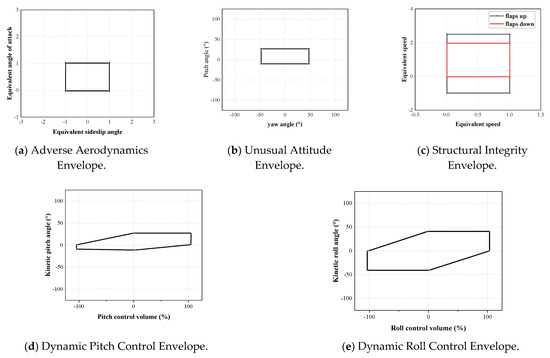
Figure 1.
LOC envelope curve [10]. (a) Adverse Aerodynamics Envelope. (b) Unusual AttitudeEnvelope. (c) Structural Integrity Envelope. (d) Dynamic Pitch Control Envelope. (e) Dynamic Roll Control Envelope.
Therefore, in order to study the protection of flight safety boundaries under icing conditions, the concept of multidimensional flight safety boundaries is introduced here. The effect of nonlinear dynamics on flight safety boundaries under icing conditions can be more accurately portrayed by constructing flight safety boundaries with multiparameter combinations [11,12,13,14,15]. The following describes the method of determining flight safety boundaries.
3. Method of Determining Flight Safety Boundaries
Usually, the industry will design the flight envelope curve according to the technical index and performance parameters satisfied by the aircraft, and verify it by means of flight tests to obtain the actual aircraft safety boundaries, such as the altitude-velocity envelope, attitude envelope, weight center of gravity envelope and maneuvering envelope of the aircraft. However, the flight test has the disadvantages of long periods, high cost, and high-risk factors [16,17,18,19,20]. For this reason, it is important to develop a high-precision flight safety boundaries determination method based on modeling and simulation calculation. Considering that the loss of control of aircraft is becoming a major cause of catastrophic accidents in aviation, scholars have carried out a lot of research work on this problem, which involves the accurate determination of dynamic boundaries in complex situations (upset conditions). By analyzing the current state of research at home and abroad, the following methods are commonly used to determine the dynamical boundaries: Bifurcation mutation theory [21], Phase plane method [22], Reachable Set estimation method [23,24,25], Stable region estimation method based on differential manifold [26], Region of Attraction (ROA) estimation method based on the sum of squares (SOS) [27], Neural Network (NN) method [28], etc. Among them, Reachable Set is favored by many scholars for its wide application and outstanding performance, and is applied in the determination of flight safety boundaries. Next, we introduce the reachable-based method for determining flight safety boundaries.
3.1. Reachable Set
The Reachable Set is widely used in security analysis. Reachable has the concepts of forward reachable and reverse reachable.
For a continuous-time nonlinear dynamical system [29]
where denotes the state variable, is the control input, is the tight set, t is the time, and is a bounded and continuous Lipschitz function, then the solution of the system exists and is unique. Here is defined as an arbitrary time range and represents the control quantity applied at time , then for any , , , the solution of the system lies on the unique solution trajectory .
Then the forward reachable can be defined as the set of states within a given initial set that can be reached within a given time range under a valid control policy , denoted by , and K is a given set of states.
Reverse reachable can be defined as the set of all states that reach the specified set of goals for a given effective control policy and time range , denoted by .
As the study of reachable set theory progressed, the concepts of maximal controllable invariant sets and invariant sets evolved. The maximum controllable invariant set is the set from which any initial state exists with at least one control input , at any given time , the track remains within the target set , denoted by .
The definition of the invariant set is more demanding than that of the maximum controllable invariant set. It is defined as any initial state from that set where the trajectory never leaves the target set at any control input and at any time . Denoted by .
The inclusive relationship between the three can be seen in Figure 2 below:
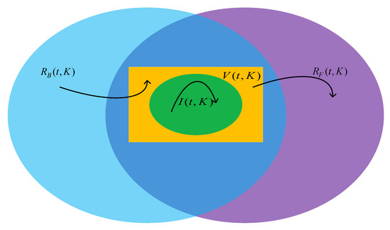
Figure 2.
Inclusion relationship between reverse reachable, invariant set, and maximum controllable invariant set [30].
From the related literature research at home and abroad, the intersection of reverse reachable, maximum controllable invariant set, invariant set, and positive and reverse reachable can be used as a kinetic safety envelope curve. Figure 2 shows the inclusion relationship between the reverse reachable, invariant set and the maximum controllable invariant set.
3.2. Real-Time Flight Simulation Platform
As seen in Figure 3, a LINKS-RT-based real-time flight simulation platform is shown. As can be seen, the simple simulation platform consists of an upper computer, a lower real-time simulator, a joystick, and a six-degree-of-freedom simulated motion cockpit. The upper computer is connected to the simulated cockpit, forwards pilot control commands to the real-time simulator via Ethernet, and converts the simulation model built on MATLAB/Simulink into C++ code supported by the lower computer’s Vxworks real-time operating system, which is deployed to the real-time simulator for execution. Flight data is also received to drive the 3D flight view simulation software and presented through the display in the simulated cockpit, forming a human-in-the-loop real-time flight simulation environment.
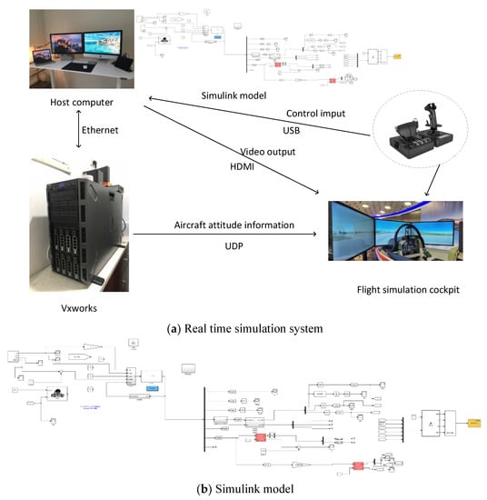
Figure 3.
Real-time flight simulation platform [31]. (a) Real time simulation system. (b) Simulink model.
3.3. Construction of 3D Geometric Digital Model of Background Aircraft Icing Configuration
Based on a comprehensive investigation of the relevant overall parameters of typical large passenger aircraft, the background aircraft plane parameters and the geometric parameters related to the size and position of the rudder surface are determined. Its basic geometric parameters are similar to those of the current large passenger aircraft of the same order as Airbus A320, Boeing 737, and C919 aircraft, and it has the basic aerodynamics and flight mechanics characteristics of large passenger aircraft. On this basis, the construction of the three-dimensional geometric digital model is completed, as shown in Figure 4.
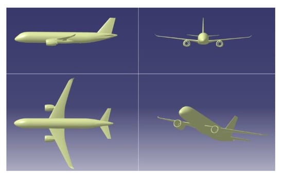
Figure 4.
Background plane three-dimensional model three-sided view.
The specific parameters of the aircraft are shown in Table 1. is Average aerodynamic chord length.

Table 1.
Related parameters of background aircraft.
3.4. Determination of Aircraft Dynamics Envelope under Icing Conditions Case
Considering the complexity in calculating the dynamical envelope of the aircraft, the dynamical characteristics of the aircraft are decoupled into longitudinal and transverse heading dynamics based on the small perturbation principle here, and the dynamical boundaries of longitudinal and transverse heading under icing conditions are calculated separately. In this paper, the maximum controllable invariant set is chosen as the kinetic envelope curve.
- Determination of longitudinal dynamics envelope of aircraft under icing conditions
Without considering the effect of the transverse heading parameter (let ), the longitudinal nonlinear dynamics equation of the aircraft can be expressed as
where: V, α and β are flight speed, angle of attack and sideslip angle, , , and are the deflection angles of the elevator, aileron, and rudder surfaces, respectively.
where: is the density of the atmosphere; S is the reference area of the wing, b is the span, is the average aerodynamic chord, is the aerodynamic force or moment coefficient, and is a function of state variables and control variables; is the derivative of the aerodynamic force or moment coefficient with respect to the state variable or manipulated variable, and is a function of the state variable and the control variable.
In order to determine the longitudinal flight safety boundaries, the HJ PDE equation needs to be solved according to the Reachable Set. One of the most important steps is to determine the envelope conditions and the optimal solution of the Hamiltonian function. Here the limits of each state parameter are given as , , , , , , , and . The input quantities are aircraft thrust and elevator deflection angle , both of which have a range of values: , , , and . Then the envelope condition can be taken as
It can be seen at , , and . K is the restricted set of state parameters.
The Hamilton function is set to
where p1, p2, p3, and p4 are the partial derivatives of with respect to states , , , and respectively.
In addition to the envelope conditions, solving the HJ PDE equation requires determining the optimal solution , , which in turn determines the safety envelope. Substituting Equation (5) into Equation (12) yields:
Then the optimal solutions and are
Once the optimal solutions and are obtained, the viscous solutions of the HJ PDE equations can be solved based on the level set algorithm to obtain the maximum controllable invariant set and thus the flight safety boundaries. Since there are four calculated state variables, the solution function is defined on . Here, for the sake of display, the calculated results are sliced by α-axis and the flight safety envelope curves are plotted for the combinations of V, q, and θ three-dimensional parameters for the clean and heavily-iced configurations calculated up to 2s under different attack angle conditions, as shown in Figure 5.
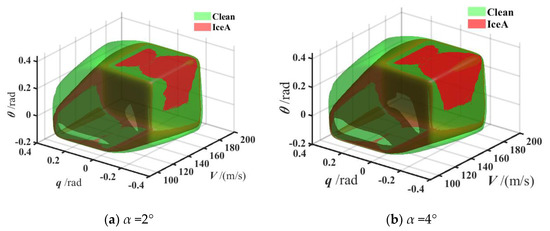
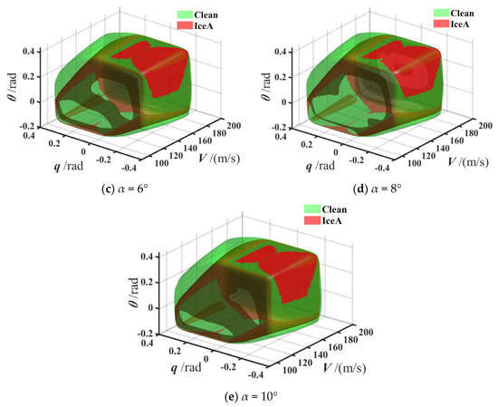
Figure 5.
Comparison of flight safety envelope curve between clean configuration and heavy icing configuration under different attack angles. (a) α = 2°, (b) α = 4°, (c) α = 6°, (d) α = 8°, (e) α = 10°.
From Figure 5, we can see that the overall change of the maximum controllable invariant set for clean and heavy icing configurations under different attack angles is not significant, which is due to the fact that the maximum controllable invariant set is a more conservative safety envelope curve, describing the set of absolute safety states of the aircraft, and non-control input variables such as attack angle do not have a significant effect on the maximum controllable invariant set. The effect of non-control input variables such as attack angle on the maximum controllable invariant set is not significant. The icing causes a shrinkage of the safety envelope curve, resulting in a reduced range of available parameters. Compared with the clean configuration, the shrinkage of the safety envelope curve of the heavy icing configuration is mainly reflected in the positive maximum region and the negative minimum region in the theta-q axes, which is due to the reduced lift, increased drag, and reduced stall attack angle of the aircraft due to icing. An excessive positive pitch angle rate is more likely to trigger a positive attack angle overrun in icing conditions, while an excessive negative pitch angle rate is more likely to trigger a negative attack angle overrun. According to the definition of the maximum controllable invariant set, for the state points in this set, it is always possible to find a control to keep the aircraft from exceeding the state limit set C. When the aircraft state points are outside the maximum controllable invariant set, it does not matter what control is used. When the aircraft state point is outside the maximum controllable invariant set, the aircraft will exceed the limit set within at most 2 s, regardless of the control used.
- 2.
- Determination of aircraft transverse heading dynamics envelope under icing conditions
The same method is used to determine the dynamical envelope of the transverse heading of the aircraft under icing conditions. Without considering the effect of the longitudinal parameters (let ), the nonlinear dynamics equation of the aircraft in the transverse direction can be expressed as:
The limits of each state parameter of the transverse heading are given here as: , , , , , , , . The input quantities are the aileron deflection angle and rudder deflection angle of the aircraft, which are taken as follows: , , , ; the thrust FT is used to keep the flight speed constant. Attack angle and pitch angle are the leveling values for the set flight state, i.e., . Then the envelope condition can be taken as:
When , and , . K is the restricted set of status parameters.
The Hamilton function is set to
where p1, p2, p3, and p4 are the partial derivatives of with respect to the states , p, r, and , respectively.
Substituting Equation (8) into Equation (10) yields
In order to obtain the maximum controllable invariant set, the optimal solutions and need to be determined. According to the above equation, the optimal solution is obtained as
The flight safety envelope curves are given here for different combinations of p, r, and 3D parameters calculated up to 2 s for different sideslip angles, as shown in Figure 6.
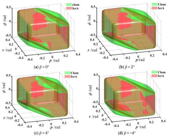
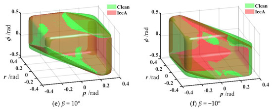
Figure 6.
Flight safety envelope curve for clean configuration/heavy-icing configuration with different sideslip angles.
From Figure 6, we can see that the safety envelope curve of both clean and heavy-icing configurations gradually shrinks with the increase of the absolute value of the sideslip angle, and both start from the region of the largest positive region and the region of the smallest negative region between the p-r axes. For the same sideslip angle, the safety envelope curve of the heavily-iced configuration shrinks significantly compared with that of the clean configuration. This is due to the change of static and dynamic stability of the transverse heading caused by icing, which makes the parameters such as p and r more likely to exceed the limits, and therefore the safety envelope shrinks.
4. L1 Adaptive Stability Augmentation Control Based on Flight Safety Boundaries Protection Method
Authors should discuss the results and how they can be interpreted from the perspective of previous studies and of the working hypotheses. The findings and their implications should be discussed in the broadest context possible. Future research directions may also be highlighted.
Based on the reconfigured flight control law of L1 adaptive stability augmentation control, an envelope protection system is designed as shown in Figure 7. In this system, the envelope protection module is designed by using command restriction, and the L1 adaptive stability augmentation control law is applied to this system to compensate for the modeling uncertainty and improve the robustness of the system, thus ensuring that the system has a normal response.
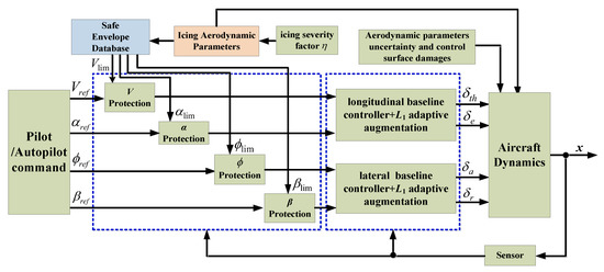
Figure 7.
Framework of icing flight safety boundaries protection system based on neural network adaptive dynamic inverse.
The main functional modules of the systems are:
- Flight safety boundaries determination module. Based on the determination method of flight safety boundaries given in the previous paper, the combination boundaries of airspeed, attack angle, sideslip angle, and roll angle are determined under different icing levels (as shown in the dashed block on the left).
- Envelope restriction protection module of critical flight parameters. This module determines the envelope limit value of key parameters given by the module according to the flight safety boundaries, and uses the command limit to achieve the protection of key safety parameters (as shown in the dashed block on the right). Take the attack angle envelope restriction as an example, the specific design method and framework of the attack angle protection module are given, as shown in Figure 8 below.
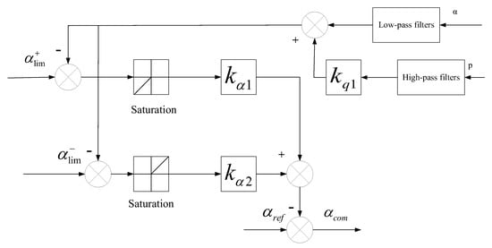 Figure 8. Attack angle envelope restriction module framework.
In Figure 7, the control principle of this module is that when the attack angle exceeds the limit value, the attack angle envelope limiting function is activated and the attack angle command value is reduced until the attack angle returns to the envelope range. The pitch angle rate q feedback is introduced in the attack angle envelope limiter to improve the system stability of the aircraft under large attack angle conditions, and the final output attack angle command is
where and are the maximum (right envelope value) and minimum (left envelope value) attack angle limits, respectively; , and are the control gains, the values of which need to be scheduled according to the flight status; is the attack angle command entered by the pilot or autopilot.
Similarly, the design principles of the envelope limitation modules for speed, sideslip angle, and roll angle are similar to those of the attack angle envelope limitation module, where the sideslip angle envelope limitation module introduces yaw angle speed r feedback to enhance system stability and the roll angle envelope limitation module introduces roll angle speed p feedback to enhance system stability. It is not repeated here.
- 3
- The flight controller module based on L1 adaptive stability augmentation control. The module takes the values of key safety parameters output from the envelope limit protection module as input commands, obtains the rudder deflection of the control rudder surface by solving the control law, and inputs them into the aircraft six-degree-of-freedom full-scale dynamics equations for calculation to obtain the dynamic response of the flight attitude and other state parameters.
5. Simulation Verification of Envelope Protection System Based on L1 Adaptive Stability Augmentation Control
In order to ensure that the critical parameters of the aircraft do not exceed the limits during the flight instructions, an envelope protection system based on L1 adaptive stability augmentation control is designed in the previous section. The following simulation is carried out to verify the effectiveness of the designed envelope protection system. The simulation system used in this paper is based on a simulation platform built by the group for the prevention and re-routing of aircraft in a classical hazard situation, and the data is obtained using the Monte Carlo method [31]. The simulation conditions are set as follows: the aircraft flies flat at an altitude of 2000 m and a speed of 100 m/s at the initial moment and encounters continuous icing, and leaves the icing region at t = 100 s. During this period, we assume that the icing severity of the aircraft increases linearly from non-icing to heavy-icing, and then remains constant. The simulation conditions are set as follows: The aircraft is maintained in level flight at an altitude of at a speed of . The aircraft encounters icing at and flies through the icing zone at . It is assumed that the severity of the aircraft icing increases linearly from non-icing to heavy-icing during this period and then remains constant. Based on the offline flight safety envelope database, the aircraft’s head angle envelope limit for this condition is correspondingly reduced linearly from . The aircraft receives a flight command from the pilot at with . Roll angle is limited to and sideslip angle is limited to . The flight speed command is set as follows: when , ; , . The flight altitude command is set as follows: when , ; , ; when , . The yaw angle command is set as follows: . The simulation time is set to 200 s. The aerodynamic parameters are also set to be time-varying during the icing process, and the specific expressions are shown in Equation (15).
The dynamic response of each parameter of the aircraft is shown in Figure 9, which is simulated without envelope protection and with envelope protection on.
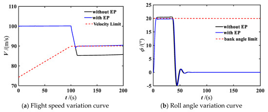
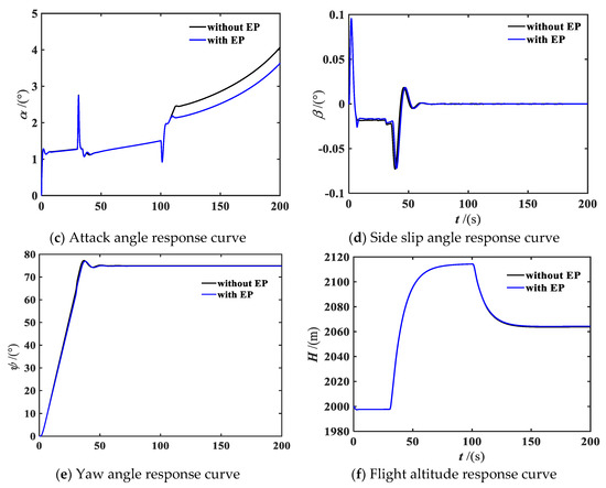
Figure 9.
Dynamic response of aircraft under envelope protection based on L1 adaptive stability augmentation control. (a) Flight speed variation curve. (b) Roll angle variation curve. (c) Attack angle response curve. (d) Side slip angle response curve. (e) Yaw angle response curve. (f) Flight altitude response curve.
Due to the effect of aircraft icing, following the flight instructions may lead to the possibility of exceeding some flight parameters of the aircraft. From Figure 8, we can see that in this simulation scenario, the flight speed and roll angle are beyond the limits when the envelope protection system is not turned on. When the envelope protection system is turned on, the flight speed and roll angle are limited to the safe range, and the precise tracking of flight commands is ensured. At the same time, the whole envelope protection system has strong robustness and can maintain a normal response under time-varying aerodynamic parameters.
Envelope Protection Test Verification based on Virtual Test Flight in Wind Tunnel
The wind tunnel virtual flight tests are carried out for the background aircraft in clean configuration and different icing simulation configurations, in which the flight control law of the background aircraft is designed using classical PID control and modern L1 adaptive control, respectively. In order to further validate the effectiveness of the L1 adaptive control-based flight safety boundaries protection system, a demonstration test of the background aircraft model boundaries protection under this modern control law configuration was carried out. The test was conducted in the artificial attitude mode, where the model was manipulated by pulling a full stick and inputting attitude angle commands to observe its response characteristics. The pre-test design of attack angle limit range is , side slip angle limit range is and roll angle limit range is , where the side slip angle limit is achieved by limiting the command range. Figure 10 gives the envelope-limiting response characteristic curves of the attitude angle of the background aircraft model under heavy-icing configuration conditions.
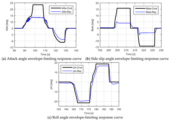
Figure 10.
Background aircraft model attitude angle envelope-limiting response characteristic curve for heavy-icing configuration. (a) Attack angle envelope-limiting response curve. (b) Side slip angle envelope-limiting response curve. (c) Roll angle envelope-limiting response curve.
As can be seen in Figure 9, the experimental results show that the envelope-limited response of attitude angle is consistent with the design effect when maneuvering with a full stick under heavy-icing configuration, and the attack angle, sideslip angle, and roll angle responses are all within the protection range. In addition, the response of the whole attitude angle is relatively smooth, but the attack angle response has a small limit ring oscillation when it is close to the stall attack angle.
In summary, the boundary protection system based on L1 adaptive stability-increasing control designed in this paper has a relatively good effect in common fault protection, compared with traditional boundary protection methods, the method proposed in this paper has the characteristics of good robustness and wide adaptation range, etc., a specific comparison is shown in Table 2.
Table 2.
Advantages and disadvantages of various protection methods.
6. Discussion
In order to achieve intelligent envelope protection for aircraft under icing conditions, this paper investigates the method of determining and protecting flight safety boundaries under icing conditions. The envelope limits of some safety critical parameters (e.g., attack angle) under icing conditions are no longer constant but are variables related to flight status and icing severity.
In order to determine the dynamic multidimensional boundaries under icing conditions, a reachable-based method for determining flight safety boundaries is proposed. The dynamic boundaries under the influence of icing as an unfavorable factor are evaluated by using the maximum controllable invariant set as the dynamic envelope curve, and the dynamic envelope curve data under the influence of multiple unfavorable factors are stored in an offline flight safety boundaries database. The calculation results show that the unfavorable factor of icing will lead to the shrinkage of the dynamics envelope curve, and the pilot needs to pay close attention to the position of the envelope curve in the flight state to prevent the aircraft from falling out of the safety envelope curve due to excessive maneuvering, which will cause flight risks.
An online flight safety boundaries protection system based on an offline database is designed. Based on the offline flight safety boundaries database, the safety envelope curve of the current flight state under icing conditions is estimated online. Based on this, the flight safety boundaries protection system based on L1 adaptive control is designed with the idea of control restriction and command restriction. Through simulation, it is verified that the proposed icing envelope protection system is fully capable of achieving the flight safety of aircraft in ice-tolerant flight situations. Compared with the traditional icing envelope protection method, the proposed method has the advantages of small computation, strong robustness, good real-time performance, and more comprehensive protection of flight parameters, which has high engineering application value.
The research in this paper can be used as a means of training pilots, and adding what has been performed in this paper to the cyber-physical systems can provide pilots with ground training experience and improve their ability to deal with the dangerous condition of icing in aircraft.
Author Contributions
Conceptualization, M.W.; methodology, Y.X.; software, M.W.; validation, M.W. and K.W.; formal analysis, M.W.; investigation, Y.X.; resources, Y.X.; data curation, K.W.; writing—original draft preparation, M.W.; writing—review and editing, Y.X.; visualization, Y.X.; supervision, Y.X.; project administration, Y.X.; funding acquisition, Y.X. All authors have read and agreed to the published version of the manuscript.
Funding
This research was funded by the National Natural Science Foundation of China, grant number 61873351.
Institutional Review Board Statement
Not applicable.
Informed Consent Statement
Not applicable.
Data Availability Statement
The data used to support the findings of this study are available from the corresponding author upon request.
Conflicts of Interest
The authors declare that there is no conflict of interest regarding the publication of this paper.
References
- Fuller, J.G.; Hook, L.R. Understanding General Aviation Accidents in Terms of Safety Systems. In Proceedings of the 39th AIAA/IEEE Digital Avionics Systems Conference (DASC), San Antonio, TX, USA, 11–15 October 2020. [Google Scholar]
- Green, N.D.C.; Ford, S.A. G-induced loss of consciousness: Retrospective survey results from 2259 military aircrew. Aviat. Space Environ. Med. 2006, 77, 619–623. [Google Scholar]
- Hess, R.A. Modeling Human Pilot Adaptation to Flight Control Anomalies and Changing Task Demands. J. Guid. Control Dyn. 2016, 39, 655–666. [Google Scholar] [CrossRef]
- Lyons, T.J.; Kraft, N.O.; Copley, G.B.; Davenport, C.; Grayson, K.; Binder, H. Analysis of mission and aircraft factors in g-induced loss of consciousness in the USAF: 1982–2002. Aviat. Space Environ. Med. 2004, 75, 479–482. [Google Scholar] [PubMed]
- Ud-Din, S.; Yoon, Y. Analysis of Loss of Control Parameters for Aircraft Maneuvering in General Aviation. J. Adv. Transp. 2018, 2018, 7865362. [Google Scholar] [CrossRef]
- Wang, K.; Xue, Y.; Tian, H.F.; Wang, M.S.; Wang, X.L. The Impact of Icing on the Airfoil on the Lift-Drag Characteristics and Maneuverability Characteristics. Math. Probl. Eng. 2021, 2021, 68740. [Google Scholar] [CrossRef]
- Wang, Y.; Shao, P.; Wu, Q.; Chen, M. Reliability analysis for a hypersonic aircraft’s wing spar. Aircr. Eng. Aerosp. Technol. 2019, 91, 549–557. [Google Scholar] [CrossRef]
- Geng, Q.; Duan, H.; Li, S. Dynamic Fault Tree Analysis Approach to Safety Analysis of Civil Aircraft. In Proceedings of the 6th IEEE Conference on Industrial Electronics and Applications (ICIEA), Beijing, China, 21–23 June 2011; pp. 1443–1448. [Google Scholar]
- Zhang, J.; Jiang, Y.; Wu, S.; Li, X.; Luo, H.; Yin, S. Prediction of remaining useful life based on bidirectional gated recurrent unit with temporal self-attention mechanism. Reliab. Eng. Syst. Saf. 2022, 221, 108297. [Google Scholar] [CrossRef]
- Belcastro, C.M.; Foster, J.V.; Shah, G.H.; Gregory, I.M.; Cox, D.E.; Crider, D.A.; Groff, L.; Newman, R.L.; Klyde, D.H. Aircraft Loss of Control Problem Analysis and Research Toward a Holistic Solution. J. Guid. Control Dyn. 2017, 40, 733–775. [Google Scholar] [CrossRef]
- Guo, K.; Liu, L.; Shi, S.; Liu, D.; Peng, X. UAV Sensor Fault Detection Using a Classifier without Negative Samples: A Local Density Regulated Optimization Algorithm. Sensors 2019, 19, 771. [Google Scholar] [CrossRef]
- Li, X.; Xu, X.; Wang, C.; Li, D. Establishment of Flight Rerouting Area and Air Route Planning based on Convex Polygon. In Proceedings of the 20th Chinese Control and Decision Conference, Yantai, China, 2–4 July 2008; pp. 3083–3088. [Google Scholar]
- Balachandran, S.; Atkins, E.M. Flight Safety Assessment and Management for Takeoff Using Deterministic Moore Machines. J. Aerosp. Inf. Syst. 2015, 12, 599–615. [Google Scholar] [CrossRef]
- Chen, D.; Luo, F.; Feng, Y. Analysis of Flight Safety Risk Coupling Based on Fuzzy Sets and Complex Network. In Proceedings of the 20th International Annual Conference on Management Science and Engineering, Harbin, China, 17–19 July 2013; pp. 329–334. [Google Scholar]
- Gan, X.-S.; Cui, H.-L.; Wu, Y.-R. Study on Mechanical Engineering for Flight with Flight Safety Evaluation Method on Relevance Vector Machine. In Proceedings of the International Conference on Mechanical Engineering, Civil Engineering and Material Engineering (MECEM 2013), Hefei, China, 27–28 October 2014; pp. 70–73. [Google Scholar]
- Gao, J.; Zhang, H.; Wang, Q.; Min, G. Safety Risk Evaluation of Aviation System Based on Fuzzy Evidential Reasoning Method. In Proceedings of the 6th International Conference on Electromechanical Control Technology and Transportation (ICECTT), Chongqing, China, 14–16 May 2022. [Google Scholar]
- Jiao, J.; Zhao, T.D.; Wang, W. Flight Safety Simulation System Based on Hybrid Dynamic System. In Proceedings of the 55th Annual Reliability and Maintainability Symposium, Ft Worth, TX, USA, 26–29 January 2009; pp. 236–242. [Google Scholar]
- Jing, H.-S.; Sheng, C.-S.; Lin, Y.-F. Flight Safety Margin Theory—A Theory for the Engineering Analysis of Flight Safety. In Proceedings of the 12th International Conference on Engineering Psychology and Cognitive Ergonomics (EPCE) Held as Part of 17th International Conference on Human-Computer Interaction (HCI International), Los Angeles, CA, USA, 2–7 August 2015; pp. 377–387. [Google Scholar]
- Lewitowicz, J.; Rutkowski, S.; Tomaska, R.; Zyluk, A. The mathematical formula of safety of aircrafts. In Proceedings of the European Safety and Reliability Conference (Esrel), Wroclaw, Poland, 14–18 September 2015; pp. 141–142. [Google Scholar]
- Li, Z.; Xu, H.; Xue, Y.; Pei, B. Study on flight safety manipulation space under complex conditions. Proc. Inst. Mech. Eng. Part G J. Aerosp. Eng. 2019, 233, 725–735. [Google Scholar] [CrossRef]
- Meng, F.; Wang, D.; Yang, P.; Xie, G.; Guo, F. Application of Sum-of-Squares Method in Estimation of Region of Attraction for Nonlinear Polynomial Systems. IEEE Access 2020, 8, 14234–14243. [Google Scholar] [CrossRef]
- Vora, A.S.; Sinha, N.K. Direct Methodology for Constrained System Analysis with Applications to Aircraft Dynamics. J. Aircr. 2017, 54, 2378–2385. [Google Scholar] [CrossRef]
- Yu, Z.; Li, Y.; Zhang, Z.; Xu, W.; Dong, Z. Online Safe Flight Envelope Protection for Icing Aircraft Based on Reachability Analysis. Int. J. Aeronaut. Space Sci. 2020, 21, 1174–1184. [Google Scholar] [CrossRef]
- Zhou, C.; Li, Y.; Zheng, W.; Wu, P.; Dong, Z. Safety Analysis for Icing Aircraft during Landing Phase Based on Reachability Analysis. Math. Probl. Eng. 2018, 2018, 3728241. [Google Scholar] [CrossRef]
- Zhou, C.; Li, Y.; Zheng, W.; Wu, P. Aircraft safety analysis based on differential manifold theory and bifurcation method. Front. Inf. Technol. Electron. Eng. 2019, 20, 292–299. [Google Scholar] [CrossRef]
- Zheng, W.; Li, Y.H.; Qu, L.; Yuan, G. Dynamic Envelope Determination Based on Differential Manifold Theory. J. Aircr. 2017, 54, 2003–2007. [Google Scholar] [CrossRef]
- Khodadadi, L.; Samadi, B.; Khaloozadeh, H. Estimation of region of attraction for polynomial nonlinear systems: A numerical method. Isa Trans. 2014, 53, 25–32. [Google Scholar] [CrossRef]
- Norouzi, R.; Kosari, A.; Sabour, M.H. Real time estimation of impaired aircraft flight envelope using feedforward neural networks. Aerosp. Sci. Technol. 2019, 90, 434–451. [Google Scholar] [CrossRef]
- Lygeros, J.; Ieee, I. On the relation of reachability to minimum cost optimal control. In Proceedings of the 41st IEEE Conference on Decision and Control, Las Vegas, NV, USA, 10–13 December 2002; pp. 1910–1915. [Google Scholar]
- Nabi, H.N.; Lombaerts, T.; Zhang, Y.; van Kampen, E.; Chu, Q.P.; de Visser, C.C. Effects of Structural Failure on the Safe Flight Envelope of Aircraft. J. Guid. Control Dyn. 2018, 41, 1257–1275. [Google Scholar] [CrossRef]
- Wei, Y.; Xu, H.; Xue, Y.; Duan, X. Quantitative assessment and visualization of flight risk induced by coupled multi-factor under icing conditions. Chin. J. Aeronaut. 2020, 33, 2146–2161. [Google Scholar] [CrossRef]


Publisher’s Note: MDPI stays neutral with regard to jurisdictional claims in published maps and institutional affiliations. |
© 2022 by the authors. Licensee MDPI, Basel, Switzerland. This article is an open access article distributed under the terms and conditions of the Creative Commons Attribution (CC BY) license (https://creativecommons.org/licenses/by/4.0/).