Equivalent Keys: Side-Channel Countermeasure for Post-Quantum Multivariate Quadratic Signatures

Abstract

Algorithms based on the hardness of solving multivariate quadratic equations present promising candidates for post-quantum digital signatures. Contemporary threats to implementations of cryptographic algorithms, especially in embedded systems, include side-channel analysis, where attacks such as differential power analysis allow for the extraction of secret keys from the device’s power consumption or its electromagnetic emission. To prevent these attacks, various countermeasures must be implemented. In this paper, we propose a novel side-channel countermeasure for multivariate quadratic digital signatures through the concept of equivalent private keys. We propose a random equivalent key to be generated prior to every signing, thus randomizing the computation and mitigating side-channel attacks. We demonstrate our approach on the Rainbow digital signature, but since an unbalanced oil and vinegar is its special case, our work is applicable to other multivariate quadratic signature schemes as well. We analyze the proposed countermeasure regarding its properties such as the number of different equivalent keys or the amount of required fresh randomness, and we propose an efficient way to implement the countermeasure. We evaluate its performance regarding side-channel leakage and time/memory requirements. Using test vector leakage assessment, we were not able to detect any statistically significant leakage from our protected implementation.

1. Introduction

In the past few decades, computer devices have become an essential part of our everyday lives. They are used throughout all industries, including banking, medicine, transportation, and entertainment. Various embedded computer systems are used to control payments, pacemakers, and trains, and most of us carry them in our own pockets every day. In the interconnected world of Industry 4.0, the Internet of Things, cloud computing, and machine learning, our privacy, security, and safety are more endangered than ever [1]. To counteract these modern-day threats, numerous security measures must be taken to provide confidentiality, authenticity, integrity, and more.

Various cryptographic primitives are widely used, including symmetric algorithms such as AES [2] and asymmetric algorithms such as RSA [3] or based on elliptic curves [4]. One of the significant threats to such asymmetric cryptographic algorithms is quantum computation, which is expected to effectively break RSA and ECC cryptosystems. This is due to Shor’s algorithm [5], which allows prime factorization and discrete logarithm solving in polynomial time, compared to exponential time on a classical computer. For this reason, the National Institute of Standards and Technology (NIST) of the United States Department of Commerce has initiated a process to standardize quantum-resistant public key cryptographic algorithms. The digital signature candidates in the third round were CRYSTALS-Dilithium [6], FALCON [7], both lattice-based schemes, and Rainbow [8], a multivariate quadratic scheme. Both lattice-based signatures have been currently recommended for standardization, with some multivariate quadratic candidate expected to be further evaluated in the fourth round. In this paper, we focus on multivariate quadratic signature schemes, which, besides Rainbow, also include the Unbalanced Oil and Vinegar (UOV) [9] and LUOV [10] schemes.

Besides classical cryptanalysis, side-channel analysis poses a threat to cryptographic implementations in general. Attacks such as differential power analysis [11] and correlation power analysis [12,13] exploit information leakage in the side-channels, such as power consumption or electromagnetic radiation [14]. More complex attacks include template attacks [15,16] and machine-learning-based attacks [17,18,19]. Successful side-channel attacks on multivariate quadratic signature schemes were presented in [20,21]. Various countermeasures against these kinds of attacks have been proposed in the literature, typically classified as either hiding or masking. Hiding countermeasures aim to conceal the leaked information in noise, e.g., by using custom secure digital logic [22,23] or additional modules such as noise generators, clock randomization, or current equalizers [24,25]. Masking countermeasures split the sensitive variable into multiple variables using random masks, thus making it difficult for the attacker to predict any intermediate values and attack. Masking countermeasures include threshold implementations [26,27] or domain-oriented masking [28]. Lightweight masking countermeasures have been proposed for multivariate cryptography, based on digest masking using a scalar mask [20,21], introducing only a little masking entropy. A more complex countermeasure, based on splitting the central map solution of Rainbow and randomizing the signing process, was presented in [29]. However, no evaluation (such as test vector leakage assessment) of the proposed countermeasures was presented in either paper. Most recently, a novel cryptanalytic attack on the Rainbow signature scheme was presented in [30], requiring reexamination of the proposed algorithm parameters and their security level.

Our Contribution

In this paper, we propose a novel side-channel countermeasure for multivariate cryptography based on private key randomization. We continue the work presented in [31] and introduce the concept of equivalent private keys, i.e., a class of private keys with the same public key. We propose a new private key to be generated prior to every signing. The adversary would then be forced to target the whole class instead of a fixed private key, making it difficult to mount a side-channel attack. We demonstrate our approach on the Rainbow algorithm. Since the UOV is a special (single-layered) case of Rainbow, our work is applicable to different multivariate cryptography algorithms as well.

We first describe the Rainbow algorithm and the notation used in Section 2. In Section 3, we introduce the general concept of equivalent keys and analyze their properties such as the number of different keys or required random bits. We further propose an efficient way to generate an equivalent key in Section 4, i.e., with fewer computational resources and randomness. Finally, we evaluate the performance of our countermeasure in Section 5 in terms of side-channel leakage and time and memory requirements. We were not able to detect any statistically significant side-channel leakage using an attack-independent test vector leakage assessment; we show that the overhead is reasonable in comparison to another state-of-the-art countermeasure.

2. Rainbow

Rainbow is a post-quantum digital signature, a generalization of the oil and vinegar signature scheme [8]. Its security depends on the fact that solving m quadratic equations for n variables becomes very difficult. These equations are defined by a central map F, which consists of multivariate quadratic polynomials. The central map is structured so that it is possible to solve $F(x_1,\dots ,x_n)=(y_1,\dots ,y_m)$ using a linear equation solver. In a public key, the special structure of the central map is hidden by two linear maps, S and T, applied on an input and an output of the central map. The central map is layered, where each layer defines two types of variables: vinegar variables for known variables (randomly generated or computed from the prior layer) and oil variables for unknown variables (to be computed using polynomials in the given layer). In this paper, we used the version of the Rainbow algorithm as defined in the submission to the NIST competition [32].

Let $\mathbb{F}$ be a finite field and $v_1,o_1,o_2\in \mathbb{N}$ the parameters of the two-layered version of Rainbow. The parameters define the number of variables and the sizes of the layers. The first layer consists of $o_1$ quadratic polynomials with $v_1$ vinegar variables with indices $V_1=\{1,2,\dots ,v_1\}$ and $o_1$ oil variables with indices $O_1=\{v_1+1,\dots ,v_1+o_1\}$. The second layer contains $o_2$ quadratic polynomials with $v_2=v_1+o_1$ vinegar variables with indices $V_2=\{1,2,\dots ,v_2\}$ and $o_2$ oil variables with indices $O_2=\{v_2+1,\dots ,v_2+o_2\}$. Overall, we have $m=o_1+o_2$ polynomials with $n=v_1+o_1+o_2$ variables.

The central map $F=(f^{(v_1+1)},f^{(v_1+2)},\dots ,f^{\left(n\right)})$ is an m-tuple of n-variate quadratic polynomials. These polynomials, indexed by $k\in O_1\cup O_2$, are defined as:

$$f^{\left(k\right)}(x_1,\dots ,x_n):=\sum _{\begin{array}{c}i,j\in V_l\\ i\le j\end{array}}{\alpha }_{i,j}^{\left(k\right)}{x}_i{x}_j+\sum _{\begin{array}{c}i\in V_l\\ j\in O_l\end{array}}{\beta }_{i,j}^{\left(k\right)}{x}_i{x}_j+\sum _{i\in V_l\cup O_l}{\gamma }_i^{\left(k\right)}{x}_i+{\delta }^{\left(k\right)},$$

(1)

where ${\alpha }_{i,j}^{\left(k\right)},{\beta }_{i,j}^{\left(k\right)},{\gamma }_i^{\left(k\right)},{\delta }^{\left(k\right)}\in \mathbb{F}$ are term coefficients and $l\in \{1,2\}$ is such that $k\in O_l$.

For simplicity, we changed the notation in Equation (1) in the following sense:

• We restricted the polynomials, omitting the linear and absolute parts of the polynomials in the central map, resulting in quadratic forms. These coefficients are not necessary for Rainbow’s security, but add more complexity. The reference implementation submitted to the standardization process considers these coefficients in the documentation, but they were not implemented in the code. Nevertheless, the countermeasure discussed in this paper can be applied to the original polynomials defined in Equation (1) as well.
• We united the $\alpha$ and $\beta$ coefficients into the $\lambda$ coefficients for simplicity of notation and also included zero coefficients as described in Equation (2). We did not allow setting any (by definition) zero coefficient to a non-zero value, so there is no change from the original definition.

  $${\lambda }_{i,j}^{\left(k\right)}:=\left\{\begin{array}{cc}{\alpha }_{i,j}^{\left(k\right)}\hfill & (k\in O_1),(i,j\in V_1),(i\le j),\hfill \\ {\beta }_{i,j}^{\left(k\right)}\hfill & (k\in O_1),(i\in V_1),(j\in O_1),\hfill \\ {\alpha }_{i,j}^{\left(k\right)}\hfill & (k\in O_2),(i,j\in V_2),(i\le j),\hfill \\ {\beta }_{i,j}^{\left(k\right)}\hfill & (k\in O_2),(i\in V_2),(j\in O_2),\hfill \\ 0\hfill & \mathrm{otherwise}.\hfill \end{array}\right.$$

  (2)

Applying our changes, we obtain a simple notation of the central map polynomials, equivalent to Equation (1):

$$f^{\left(k\right)}\left(\mathbf{x}\right)=\sum _{i,j\in \widehat{n}}{\lambda }_{i,j}^{\left(k\right)}·x_i·x_j,$$

(3)

where $k\in O_1\cup O_2,\widehat{n}=\{1,2,\dots ,n\}$ and $\mathbf{x}=(x_1,\dots ,x_n)$.

In Rainbow, the structure of the central map F (described in Equation (1)) is hidden using two random invertible affine maps $S:{\mathbb{F}}^m\to {\mathbb{F}}^m$ and $T:{\mathbb{F}}^n\to {\mathbb{F}}^n$. Similar to the linear and absolute parts of the central map polynomials, we also omitted translations of the affine maps. Therefore, we used two linear maps represented by regular matrices $\mathbf{S}\in {\mathbb{F}}^{m\times m},\mathbf{T}\in {\mathbb{F}}^{n\times n}$. This is also consistent with the reference implementation.

2.1. Central Map in Matrix Representation

For compact writing, we rewrite the quadratic forms in the central map as a product of matrix–vector multiplication for $k\in O_1\cup O_2$:

$$\begin{array}{cc}\hfill f^{\left(k\right)}\left(\mathbf{x}\right)& ={\mathbf{x}}^{⊺}{\mathbf{F}}^{\left(k\right)}\mathbf{x}={\mathbf{x}}^{⊺}\left(\begin{array}{ccc}{\mathbf{F}}_{1,1}^{\left(k\right)}& {\mathbf{F}}_{1,2}^{\left(k\right)}& {\mathbf{F}}_{1,3}^{\left(k\right)}\\ \mathbf{0}& {\mathbf{F}}_{2,2}^{\left(k\right)}& {\mathbf{F}}_{2,3}^{\left(k\right)}\\ \mathbf{0}& \mathbf{0}& \mathbf{0}\end{array}\right)\mathbf{x},\hfill \\ \hfill {\mathbf{F}}_{1,1}^{\left(k\right)}& ={\left\{{\lambda }_{i,j}^{\left(k\right)}\right\}}_{i,j\in V_1},\hfill \\ \hfill {\mathbf{F}}_{1,2}^{\left(k\right)}& ={\left\{{\lambda }_{i,j}^{\left(k\right)}\right\}}_{i\in V_1,j\in O_1},\hfill \\ \hfill {\mathbf{F}}_{1,3}^{\left(k\right)}& ={\left\{{\lambda }_{i,j}^{\left(k\right)}\right\}}_{i\in V_1,j\in O_2},\hfill \\ \hfill {\mathbf{F}}_{2,2}^{\left(k\right)}& ={\left\{{\lambda }_{i,j}^{\left(k\right)}\right\}}_{i,j\in O_1},\hfill \\ \hfill {\mathbf{F}}_{2,3}^{\left(k\right)}& ={\left\{{\lambda }_{i,j}^{\left(k\right)}\right\}}_{i\in O_1,j\in O_2}.\hfill \end{array}$$

(4)

The quadratic form $f^{\left(k\right)}\left(\mathbf{x}\right)$ can be expressed using a matrix ${\mathbf{F}}^{\left(k\right)}$. This matrix is partitioned according to the structure of the central map. Submatrices ${\mathbf{F}}_{1,1}^{\left(k\right)},{\mathbf{F}}_{2,2}^{\left(k\right)}$ are upper triangulars and correspond to alpha coefficients. Submatrices ${\mathbf{F}}_{1,2}^{\left(k\right)},{\mathbf{F}}_{1,3}^{\left(k\right)},{\mathbf{F}}_{2,3}^{\left(k\right)}$ correspond to beta coefficients. Specifically for the first layer, we obtain:

$$(k\in O_1)\Rightarrow {\mathbf{F}}^{\left(k\right)}=\left(\begin{array}{ccc}{\mathbf{F}}_{1,1}^{\left(k\right)}& {\mathbf{F}}_{1,2}^{\left(k\right)}& \mathbf{0}\\ \mathbf{0}& \mathbf{0}& \mathbf{0}\\ \mathbf{0}& \mathbf{0}& \mathbf{0}\end{array}\right).$$

(5)

The central map can be expressed as a vector of m matrices (representing quadratic forms):

$$\mathbf{F}=\left(\begin{array}{c}{\mathbf{F}}^{(v_1+1)}\\ {\mathbf{F}}^{(v_1+2)}\\ ⋮\\ {\mathbf{F}}^{\left(n\right)}\end{array}\right).$$

(6)

Secret key SK can be expressed and stored as:

$$\mathrm{SK}=(S^{-1},F,T^{-1})\leftrightarrow ({\mathbf{S}}^{-1},\mathbf{F},{\mathbf{T}}^{-1}),$$

(7)

where

$$\begin{array}{cc}\hfill F:& {\mathbb{F}}^n\to {\mathbb{F}}^m\hfill \\ \hfill & \mathbf{x}\mapsto y=F\left(\mathbf{x}\right)=\left(\begin{array}{c}{f}^{(v_1+1)}\left(\mathbf{x}\right)\\ f^{(v_1+2)}\left(\mathbf{x}\right)\\ ⋮\\ f^{\left(n\right)}\left(\mathbf{x}\right)\end{array}\right)=\left(\begin{array}{c}{\mathbf{x}}^{⊺}{\mathbf{F}}^{(v_1+1)}\mathbf{x}\\ {\mathbf{x}}^{⊺}{\mathbf{F}}^{(v_1+2)}\mathbf{x}\\ ⋮\\ {\mathbf{x}}^{⊺}{\mathbf{F}}^{\left(n\right)}\mathbf{x}\end{array}\right).\hfill \end{array}$$

(8)

The public key contains only a quadratic map P defined as

$$P:=S\circ F\circ T.$$

(9)

2.2. Signing and Verification Process

For document $\mathbf{d}$, random salt $\mathbf{r}$, and a secret key $\mathrm{SK}=(S^{-1},F,T^{-1})$, we define

$$\begin{array}{cc}\hfill \mathbf{h}:=& \mathrm{hash}\left(\mathrm{hash}\left(\mathbf{d}\right)\left|\right|\mathbf{r}\right),\hfill \\ \hfill \mathbf{y}:=& S^{-1}\left(\mathbf{h}\right),\hfill \\ \hfill \mathbf{x}:=& F^{-1}\left(\mathbf{y}\right),\hfill \\ \hfill \mathbf{z}:=& T^{-1}\left(\mathbf{x}\right),\hfill \end{array}$$

(10)

where $\mathbf{h},\mathbf{y}\in {\mathbb{F}}^m$ and $\mathbf{x},\mathbf{z}\in {\mathbb{F}}^n$. The pair $(\mathbf{z},\mathbf{r})$ is called a signature.

The signature $(\mathbf{z},\mathbf{r})$ of the document $\mathbf{d}$ is valid iff $\mathbf{h}={\mathbf{h}}^{\prime }$, where

$$\begin{array}{cc}\hfill \mathbf{h}:=& \mathrm{hash}\left(\mathrm{hash}\left(\mathbf{d}\right)\left|\right|\mathbf{r}\right),\hfill \\ \hfill {\mathbf{h}}^{\prime }:=& P\left(\mathbf{z}\right).\hfill \end{array}$$

(11)

3. Equivalent Key

The main idea of the equivalent key is to change the secret key SK into some other $\overline{\mathrm{SK}}$, which is equivalent to the original one, i.e., SK and $\overline{\mathrm{SK}}$ both have the same public key. This equivalency was previously used for storage, computation, and randomness reduction, where only the normal form of the key was generated [31]. Our countermeasure is based on the generation of the equivalent key before each signing process. We therefore substituted a fixed key with an equivalence class containing a huge number (as shown in Equation (28)) of different, but equivalent, keys.

In our work, the equivalent key can be derived from the original key using two linear maps A and B, represented as matrices $\mathbf{A}$ and $\mathbf{B}$, which change all three maps contained in a secret key without changing their composition:

$$\begin{array}{cc}\hfill P& =S\circ F\circ T,\hfill \\ \hfill P& =S\circ (A^{-1}\circ A)\circ F\circ (B\circ B^{-1})\circ T,\hfill \\ \hfill P& =(S\circ A^{-1})\circ (A\circ F\circ B)\circ (B^{-1}\circ T).\hfill \end{array}$$

(12)

With this in mind, we define the secret key $\overline{\mathrm{SK}}$ derived from SK as

$$\begin{array}{cc}\hfill \mathrm{SK}& =(S^{-1},F,T^{-1}),\hfill \\ \hfill \overline{\mathrm{SK}}& =(A\circ S^{-1},A\circ F\circ B,T^{-1}\circ B).\hfill \end{array}$$

(13)

The pair $(A,B)$ is called Gauss sustaining transformation, where the representing matrices $\mathbf{A}$ and $\mathbf{B}$ cannot be chosen arbitrarily. They are composed with the central map F, which must maintain its special structure.

The necessary constraint is the invertibility of these matrices due to the signing process, where the inverse central map must be computed. Therefore, $\mathbf{A}$ and $\mathbf{B}$ must be regular; thus, $\det \left(\mathbf{A}\right)\ne 0$ and $\det \left(\mathbf{B}\right)\ne 0$. The compositions $A\circ S^{-1}$ and $T^{-1}\circ B$ can be computed simply as $\mathbf{A}{\mathbf{S}}^{-1}$ and ${\mathbf{T}}^{-1}\mathbf{B}$. The composition $A\circ F\circ B$ is discussed in the following sections.

3.1. Composition $A\circ F$

Let $A:{\mathbb{F}}^m\to {\mathbb{F}}^m,\mathbf{h}\mapsto A\left(\mathbf{h}\right)=\mathbf{A}\mathbf{h}$, where $\mathbf{A}\in {\mathbb{F}}^{m\times m}$ is a regular matrix. The composition $A\circ F$ is then

$$(A\circ F)\left(\mathbf{x}\right)=\mathbf{A}\left(\begin{array}{c}{f}^{(v_1+1)}\left(\mathbf{x}\right)\\ f^{(v_1+2)}\left(\mathbf{x}\right)\\ ⋮\\ f^{\left(n\right)}\left(\mathbf{x}\right)\end{array}\right)=\left(\begin{array}{c}\sum _{i=1}^m{A}_{1,i}{f}^{(v_1+i)}\left(\mathbf{x}\right)\\ \sum _{i=1}^m{A}_{2,i}{f}^{(v_1+i)}\left(\mathbf{x}\right)\\ ⋮\\ \sum _{i=1}^m{A}_{m,i}{f}^{(v_1+i)}\left(\mathbf{x}\right)\end{array}\right),$$

(14)

and $\forall k\in \{1,\dots ,m\}:$

$${[A\circ F]}_k\left(\mathbf{x}\right)=\sum _{i=1}^m{A}_{k,i}·f^{(v_1+i)}\left(\mathbf{x}\right)=\sum _{i=1}^m{A}_{k,i}·\left({\mathbf{x}}^{⊺}{\mathbf{F}}^{(v_1+i)}\mathbf{x}\right)={\mathbf{x}}^{⊺}\sum _{i=1}^m(A_{k,i}·{\mathbf{F}}^{(v_1+i)})\mathbf{x}.$$

(15)

The composition is equivalent to a linear combination of $\mathbf{F}$ matrices. In the following equation, we show how arbitrary $\mathbf{A}$ affects the structure of the central map:

$$\sum _{i=1}^m{A}_{k,i}·{\mathbf{F}}^{(v_1+i)}=\sum _{i=1}^m{A}_{k,i}·\left(\begin{array}{ccc}{\mathbf{F}}_{1,1}^{(v_1+i)}& {\mathbf{F}}_{1,2}^{(v_1+i)}& {\mathbf{F}}_{1,3}^{(v_1+i)}\\ \mathbf{0}& {\mathbf{F}}_{2,2}^{(v_1+i)}& {\mathbf{F}}_{2,3}^{(v_1+i)}\\ \mathbf{0}& \mathbf{0}& \mathbf{0}\end{array}\right).$$

(16)

To maintain the special structure for the first layer ($k\in \{1,\dots ,o_1\}$), as described in Equation (5), we must fulfill the following restrictions:

$$\begin{array}{cc}\hfill \sum _{i=1}^m{A}_{k,i}·{\mathbf{F}}_{1,3}^{(v_1+i)}& =\mathbf{0},\hfill \\ \hfill \sum _{i=1}^m{A}_{k,i}·{\mathbf{F}}_{2,2}^{(v_1+i)}& =\mathbf{0},\hfill \\ \hfill \sum _{i=1}^m{A}_{k,i}·{\mathbf{F}}_{2,3}^{(v_1+i)}& =\mathbf{0}.\hfill \end{array}$$

(17)

Since, $\forall i\in O_1:{\mathbf{F}}_{1,3}^{\left(i\right)},{\mathbf{F}}_{2,2}^{\left(i\right)},{\mathbf{F}}_{2,3}^{\left(i\right)}$ are zero matrices, Equation (17) can be rewritten as

$$\begin{array}{cc}\hfill \sum _{i=o_1+1}^m{A}_{k,i}·{\mathbf{F}}_{1,3}^{(v_1+i)}& =\mathbf{0},\hfill \\ \hfill \sum _{i=o_1+1}^m{A}_{k,i}·{\mathbf{F}}_{2,2}^{(v_1+i)}& =\mathbf{0},\hfill \\ \hfill \sum _{i=o_1+1}^m{A}_{k,i}·{\mathbf{F}}_{2,3}^{(v_1+i)}& =\mathbf{0}.\hfill \end{array}$$

(18)

This restriction can be trivially satisfied by the following condition:

$$(\forall k\in \{1,\dots ,o_1\})(\forall i\in \{o_1+1,\dots ,m\}):A_{k,i}=0.$$

(19)

Regarding the second layer, the arbitrary A maintains its polynomial structure by itself, and therefore, no further restrictions are necessary.

An applicable matrix $\mathbf{A}\in {\mathbb{F}}^{m\times m}$ is therefore

$$\mathbf{A}=\left(\begin{array}{cc}{\mathbf{A}}_{1,1}& \mathbf{0}\\ {\mathbf{A}}_{2,1}& {\mathbf{A}}_{2,2}\end{array}\right),$$

(20)

where ${\mathbf{A}}_{1,1}\in {\mathbb{F}}^{o_1\times o_1},{\mathbf{A}}_{2,1}\in {\mathbb{F}}^{o_2\times o_1},{\mathbf{A}}_{2,2}\in {\mathbb{F}}^{o_2\times o_2}$. Matrix $\mathbf{A}$ must be regular; therefore, ${\mathbf{A}}_{1,1}$ and ${\mathbf{A}}_{2,2}$ are arbitrary regular matrices and ${\mathbf{A}}_{1,2}$ is an (possibly singular) arbitrary matrix.

From the matrix $\mathbf{A}$, we deduce that the linear combination is performed separately in layers (${\mathbf{A}}_{1,1}$ and ${\mathbf{A}}_{2,2}$), and quadratic polynomials from the first layer can be combined into the second layer (${\mathbf{A}}_{2,1}$).

3.2. Composition $F\circ B$

Let $B:{\mathbb{F}}^n\to {\mathbb{F}}^n,\mathbf{x}\mapsto B\left(\mathbf{x}\right)=\mathbf{B}\mathbf{x}$, where $\mathbf{B}\in {\mathbb{F}}^{n\times n}$ is a regular matrix. The composition $F\circ B$ is then

$$(F\circ B)\left(\mathbf{x}\right)=F\circ \left(\mathbf{B}\mathbf{x}\right)=\left(\begin{array}{c}{f}^{(v_1+1)}\left(\mathbf{B}\mathbf{x}\right)\\ f^{(v_1+2)}\left(\mathbf{B}\mathbf{x}\right)\\ ⋮\\ f^{\left(n\right)}\left(\mathbf{B}\mathbf{x}\right)\end{array}\right),$$

(21)

and, $\forall k\in \{1,\dots ,m\}$:

$${\left[(F\circ B)\right]}_k\left(\mathbf{x}\right)=f^{(v_1+k)}\left(\mathbf{B}\mathbf{x}\right)={\left(\mathbf{B}\mathbf{x}\right)}^{⊺}{\mathbf{F}}^{(v_1+k)}\mathbf{B}\mathbf{x}={\mathbf{x}}^{⊺}\left({\mathbf{B}}^{⊺}{\mathbf{F}}^{(v_1+k)}\mathbf{B}\right)\mathbf{x}.$$

(22)

This composition changes every quadratic polynomial separately. Before we consider the restrictions on the matrix $\mathbf{B}$, let us first introduce the following lemma.

Lemma 1.

Every quadratic form can be represented as an upper triangular matrix.

Proof. 

Let $q\in \mathbb{F}\left[\mathbf{x}\right]$ be a quadratic form represented by matrix $\mathcal{Q}$, then $\mathcal{U}$ is an upper triangular representation of q, where $\mathcal{U}$ is

$$\begin{array}{c}\hfill \forall i,j\in \{1,\dots ,n\}:{\mathcal{U}}_{i,j}=\left\{\begin{array}{cc}{\mathcal{Q}}_{i,i}\hfill & i=j,\hfill \\ {\mathcal{Q}}_{i,j}+{\mathcal{Q}}_{j,i}\hfill & i<j,\hfill \\ 0\hfill & \mathrm{otherwise}.\hfill \end{array}\right.\end{array}$$

(23)

Then,

$$q\left(\mathbf{x}\right)={\mathbf{x}}^{⊺}\mathcal{Q}\mathbf{x}=\sum _{i,j\in \{1,\dots ,n\}}{\mathcal{Q}}_{i,j}{x}_i{x}_j=\sum _{i\in \{1,\dots ,n\}}{\mathcal{Q}}_{i,i}{x}_i^2+\sum _{\begin{array}{c}i,j\in \{1,\dots ,n\}\\ i<j\end{array}}({\mathcal{Q}}_{i,j}+{\mathcal{Q}}_{j,i})x_i{x}_j={\mathbf{x}}^{⊺}\mathcal{U}\mathbf{x}.$$

(24)

   □

Let $◹:{\mathbb{F}}^{n\times n}\to {\mathbb{F}}^{n\times n};\mathcal{Q}\mapsto \mathcal{U}$ be a function, where $\mathcal{U}$ is an upper triangular matrix, such that $\forall \mathbf{x}\in {\mathbb{F}}^n:{\mathbf{x}}^{⊺}\mathcal{Q}\mathbf{x}={\mathbf{x}}^{⊺}\mathcal{U}\mathbf{x}$.

In Equation (25), we show how matrix $\mathbf{B}$ changes the structure of a polynomial in the central map. We used the same partitioning of the matrix $\mathbf{B}$ as we used for the matrix ${\mathbf{F}}^{\left(k\right)}$. Size compatibility for the matrix multiplication is guaranteed thanks to the symmetry of block sizes. We further applied the function $◹$, as it does not change the concerned polynomial and it helps us with the wanted structure. It ensures the upper triangular submatrices on the diagonal, which are required by the definition of Rainbow.

$$\begin{array}{cc}\hfill \mathbf{B}& =\left(\begin{array}{ccc}{\mathbf{B}}_{1,1}& {\mathbf{B}}_{1,2}& {\mathbf{B}}_{1,3}\\ {\mathbf{B}}_{2,1}& {\mathbf{B}}_{2,2}& {\mathbf{B}}_{2,3}\\ {\mathbf{B}}_{3,1}& {\mathbf{B}}_{3,2}& {\mathbf{B}}_{3,3}\end{array}\right),\hfill \\ \hfill k\in O_1:◹\left({\mathbf{B}}^{⊺}{\mathbf{F}}^{\left(k\right)}\mathbf{B}\right)& =\left(\begin{array}{ccc}{\mathbf{F}}_{1,1}^{\prime \left(k\right)}& {\mathbf{F}}_{1,2}^{\prime \left(k\right)}& \mathbf{0}\\ \mathbf{0}& \mathbf{0}& \mathbf{0}\\ \mathbf{0}& \mathbf{0}& \mathbf{0}\end{array}\right),\hfill \\ \hfill k\in O_2:◹\left({\mathbf{B}}^{⊺}{\mathbf{F}}^{\left(k\right)}\mathbf{B}\right)& =\left(\begin{array}{ccc}{\mathbf{F}}_{1,1}^{\prime \left(k\right)}& {\mathbf{F}}_{1,2}^{\prime \left(k\right)}& {\mathbf{F}}_{1,3}^{\prime \left(k\right)}\\ \mathbf{0}& {\mathbf{F}}_{2,2}^{\prime \left(k\right)}& {\mathbf{F}}_{2,3}^{\prime \left(k\right)}\\ \mathbf{0}& \mathbf{0}& \mathbf{0}\end{array}\right).\hfill \end{array}$$

(25)

Solving this system of equations with matrix $\mathbf{B}$ as a variable for arbitrary central map $\mathbf{F}$, where the right sides of the equations are zeroes, we obtain:

$$\mathbf{B}=\left(\begin{array}{ccc}{\mathbf{B}}_{1,1}& \mathbf{0}& \mathbf{0}\\ {\mathbf{B}}_{2,1}& {\mathbf{B}}_{2,2}& \mathbf{0}\\ {\mathbf{B}}_{3,1}& {\mathbf{B}}_{3,2}& {\mathbf{B}}_{3,3}\end{array}\right),$$

(26)

where non-zero submatrices are arbitrary submatrices, except that matrix $\mathbf{B}$ must be regular, and therefore, submatrices ${\mathbf{B}}_{1,1},{\mathbf{B}}_{2,2},{\mathbf{B}}_{3,3}$ must be regular.

For an insight into what is happening to the vector $\mathbf{x}$ (which elements are the variables in the central map), we can partition $\mathbf{x}$ into three different types of variables: vinegar variables of the first layer (${\mathbf{x}}_1^v\in {\mathbb{F}}^{v_1}$), oil variables of the first layer (${\mathbf{x}}_1^o\in {\mathbb{F}}^{o_1}$), and oil variables of the second layer (${\mathbf{x}}_2^o\in {\mathbb{F}}^{o_2}$). If we apply matrix $\mathbf{B}$ to the vector $\mathbf{x}$, we obtain:

$$\mathbf{B}\mathbf{x}=\left(\begin{array}{ccc}{\mathbf{B}}_{1,1}& \mathbf{0}& \mathbf{0}\\ {\mathbf{B}}_{2,1}& {\mathbf{B}}_{2,2}& \mathbf{0}\\ {\mathbf{B}}_{3,1}& {\mathbf{B}}_{3,2}& {\mathbf{B}}_{3,3}\end{array}\right)\left(\begin{array}{c}{\mathbf{x}}_1^v\\ {\mathbf{x}}_1^o\\ {\mathbf{x}}_2^o\end{array}\right)=\left(\begin{array}{c}{\mathbf{B}}_{1,1}{\mathbf{x}}_1^v\\ {\mathbf{B}}_{2,1}{\mathbf{x}}_1^v+{\mathbf{B}}_{2,2}{\mathbf{x}}_1^o\\ {\mathbf{B}}_{3,1}{\mathbf{x}}_1^v+{\mathbf{B}}_{3,2}{\mathbf{x}}_1^o+{\mathbf{B}}_{3,3}{\mathbf{x}}_2^o\end{array}\right).$$

(27)

In this situation, the variables to solve are not defined only by vector $\mathbf{x}$, but the vector $\mathbf{B}\mathbf{x}$. To be able to sign, it is necessary not to mix the vinegar variable with the oil variables of each layer. At the beginning of the signing process, we used ${\mathbf{B}}_{1,1}{\mathbf{x}}_1^v$ instead of ${\mathbf{x}}_1^v$. Vector ${\mathbf{x}}_1^v$ is randomly generated, thus known. We can easily compute ${\mathbf{B}}_{1,1}{\mathbf{x}}_1^v$. Next, the first layer is solved, where we computed ${\mathbf{B}}_{2,1}{\mathbf{x}}_1^v+{\mathbf{B}}_{2,2}{\mathbf{x}}_1^o$ instead of ${\mathbf{x}}_1^o$. We can immediately substitute ${\mathbf{B}}_{2,1}{\mathbf{x}}_1^v$, which is already known. We still obtain a system of the linear equations that has only variables of the vector ${\mathbf{x}}_1^o$. In the end, the second layer is solved. We can first substitute ${\mathbf{B}}_{3,1}{\mathbf{x}}_1^v+{\mathbf{B}}_{3,2}{\mathbf{x}}_1^o$, and again, we obtain only a system of linear equations. No oil and vinegar variables (of the same layer) are mixed. This was only an insight into why the inversion of the central map can be still computed. In the implementation, matrix $\mathbf{B}$ is incorporated in the central map (as a generator of the equivalent key).

3.3. Analysis of an Equivalent Key

In this section, we discuss the basic properties of the equivalent key. We concentrate only on equivalent keys that can be generated according to Equation (13), with the maps A and B defined in Equation (20) and Equation (26). We start with the number of equivalent keys, and we calculate entropy where applicable. Then, we state the benefits of our masking scheme. For the analysis in this section, we considered two sets of Rainbow parameters:

• Ia (128 bit security): ${\mathbb{F}}_q=GF\left(16\right),v_1=36,o_1=o_2=32$;
• Vc (256 bit security): ${\mathbb{F}}_q=GF\left(256\right),v_1=96,o_1=36$ and $o_2=64$.

We note that these parameters, while suggested in the NIST standardization process, are probably already inadequate due to the recently presented attacks [30].

Lemma 2.

Let $M_{l,s}\left({\mathbb{F}}_q\right)=\{l\times smatricesover{\mathbb{F}}_q\}$ be a set. The cardinality of the set is $|M_{l,s}\left({\mathbb{F}}_q\right)|=q^{l·s}$.

Lemma 3.

Let $M_n\left({\mathbb{F}}_q\right)=\{n\times nmatricesover{\mathbb{F}}_q\}$, with the matrix multiplication, be the full linear monoid. The order of the monoid is $|M_n\left({\mathbb{F}}_q\right)|=q^{n^2}$.

Lemma 4.

Let $G{L}_n\left({\mathbb{F}}_q\right)=\{n\times ninvertiblematricesover{\mathbb{F}}_q\}$, with the matrix multiplication, be the general linear group. The order is $|G{L}_n\left({\mathbb{F}}_q\right)|={\prod }_{k=0}^{n-1}(q^n-q^k)=q^{n^2}{(q^{-n};q)}_n$. (q-Pochhammer symbol: ${(a;q)}_n:={\prod }_{k=0}^{n-1}(1-a{q}^k),n>0$, defined inter alia in [33]. For example: the number of $10\times 10$ regular matrices over $\mathrm{GF}\left(16\right)$ is $|G{L}_{10}\left({\mathbb{F}}_{16}\right)|\approx 0.9336·{16}^{100}$, where ${({16}^{-10};16)}_{10}\approx 0.9336$. Symbol ${(q^{-n},q)}_n$ denotes the ratio between regular matrices $n\times n$ and all matrices $n\times n$ over ${\mathbb{F}}_q$.)

The proofs of these three lemmas are well known [34].

Theorem 1.

The number of different equivalent keys, over a fixed secret key SK, is

$$q^{v_1(v_1+o_1+o_2)+2(o_1^2+o_1{o}_2+o_2^2)}{(q^{-v_1};q)}_{v_1}{\left({(q^{-o_1};q)}_{o_1}\right)}^2{\left({(q^{-o_2};q)}_{o_2}\right)}^2.$$

(28)

This is an exact number, where the left part $q^{(\dots )}$ describes the number of different combinations of matrices $\mathbf{A}$ and $\mathbf{B}$. The remaining part counts for the cases where $\mathbf{A}$ and $\mathbf{B}$ are regular. For $\mathrm{GF}\left(16\right)$, its value is $\approx 0.7092$, and for $\mathrm{GF}\left(256\right)$ it is $\approx 0.9805$. This value is dependent on the values $v_1,o_1,o_2$, but it converges with these parameters extremely fast. For $\mathrm{GF}\left(16\right)$, the difference between $v_1=o_1=o_2=10$ and $v_1=o_1=o_2=1000$ is less then ${10}^{-12}$.

Proof. (Number of different equivalent keys) We show that the number of equivalent keys is the number of possible non-equal matrices $\mathbf{A}$ multiplied by the number of possible non-equal matrices $\mathbf{B}$. This holds because both matrices are applied to different parts of the secret key (maps S and T), so they cannot interfere with each other, and they are both generated independently. We discuss the number of keys for matrix $\mathbf{A}$ only, and the same procedure can be applied to matrix $\mathbf{B}$. Let $\mathbb{A}$ be the set of matrices with the structure defined in Equation (20) and a regular matrix $\mathbf{S}\in {\mathrm{GL}}_m\left({\mathbb{F}}_q\right)$ be the representation of the linear map S.

First, we show that the lower bound of the number of equivalent keys generated by $\mathbb{A}$ is equal to the cardinality of the set $\mathbb{A}$. This is because a regular matrix $\mathbf{S}$ is multiplied by regular matrices from the set $\mathbb{A}$. Thus, two distinct matrices $\mathbf{A},{\mathbf{A}}^{\prime }\in \mathbb{A}\subset \mathrm{GL}$ cannot generate the same product matrix:

$$\forall \mathbf{A},{\mathbf{A}}^{\prime }\in {\mathrm{GL}}_m\left({\mathbb{F}}_q\right):\mathbf{A}\ne {\mathbf{A}}^{\prime }\Rightarrow \mathbf{A}\mathbf{S}\ne {\mathbf{A}}^{\prime }\mathbf{S}.$$

(29)

Therefore, each distinct matrix in $\mathbb{A}$ generates a different equivalent key; hence, the cardinality of the set $\mathbb{A}$ is the lower bound of the number of different equivalent keys generated by $\mathbb{A}$.

Second, we show that the cardinality of the set $\mathbb{A}$ is also the upper bound of the number of different equivalent keys generated by $\mathbb{A}$, since every equivalent key can be reached by a multiplication with a single $\mathbf{A}\in \mathbb{A}$. Let us examine a product of two matrices $\mathbf{A},{\mathbf{A}}^{\prime }\in \mathbb{A}$:

$$\mathbf{A}{\mathbf{A}}^{\prime }=\left(\begin{array}{cc}{\mathbf{A}}_{1,1}{\mathbf{A}}_{1,1}^{\prime }& \mathbf{0}\\ {\mathbf{A}}_{2,1}{\mathbf{A}}_{1,1}^{\prime }+{\mathbf{A}}_{2,2}{\mathbf{A}}_{2,1}^{\prime }& {\mathbf{A}}_{2,2}{\mathbf{A}}_{2,2}^{\prime }\end{array}\right).$$

(30)

The matrix $\mathbf{A}{\mathbf{A}}^{\prime }$ has the same structure as the matrices $\mathbf{A}$ and ${\mathbf{A}}^{\prime }$. On the diagonal, we have the products of the elements of $\mathrm{GL}$, which also result in an element of the $\mathrm{GL}$, and the submatrix ${\left[\mathbf{A}{\mathbf{A}}^{\prime }\right]}_{2,1}$ can be an arbitrary matrix, thus $\mathbf{A}{\mathbf{A}}^{\prime }\in \mathbb{A}$. In other words, every key reachable by subsequent multiplications with two matrices from $\mathbb{A}$ can be reached by a single multiplication with some matrix from $\mathbb{A}$:

$$(\forall \mathbf{A},{\mathbf{A}}^{\prime }\in \mathbb{A})(\exists {\mathbf{A}}^{″}\in \mathbb{A}):{\mathbf{A}}^{\prime }\left(\mathbf{A}\mathbf{S}\right)={\mathbf{A}}^{″}\mathbf{S}.$$

(31)

Therefore, the upper bound of the number of equivalent keys generated by $\mathbb{A}$ is the size of the set $\mathbb{A}$.

The previous statements imply that the number of equivalent keys generated by $\mathbb{A}$ is equal to the size of the set $\mathbb{A}$. Every matrix $\mathbf{A}\in \mathbb{A}$ has four parts: two submatrices from GL, one from $M_{o_1,o_2}\left({\mathbb{F}}_q\right)$, and a zero submatrix. All matrices are independent, so the total number of matrices is the product of the numbers of different submatrices:

$$\begin{array}{cc}\hfill & |{\mathrm{GL}}_{o_1}\left({\mathbb{F}}_q\right)|·|{\mathrm{GL}}_{o_2}\left({\mathbb{F}}_q\right)|·|M_{o_1,o_2}\left({\mathbb{F}}_q\right)|·1=\hfill \\ \hfill & =q^{(o_1^2+o_2^2+o_1{o}_2)}{(q^{-o_1};q)}_{o_1}{(q^{-o_2};q)}_{o_2}.\hfill \end{array}$$

(32)

The number of different matrices $\mathbf{B}$ can be computed in a similar fashion:

$$\begin{array}{cc}\hfill & |{\mathrm{GL}}_{v_1}\left({\mathbb{F}}_q\right)|·|{\mathrm{GL}}_{o_1}\left({\mathbb{F}}_q\right)|·|{\mathrm{GL}}_{o_2}\left({\mathbb{F}}_q\right)|·|M_{v_1,o_1}\left({\mathbb{F}}_q\right)|·|M_{v_1,o_2}\left({\mathbb{F}}_q\right)|·|M_{o_1,o_2}\left({\mathbb{F}}_q\right)|=\hfill \\ \hfill & =q^{(v_1^2+o_1^2+o_2^2+v_1{o}_1+v_1{o}_2+o_1{o}_2)}{(q^{-v_1};q)}_{v_1}{(q^{-o_1};q)}_{o_1}{(q^{-o_2};q)}_{o_2}.\hfill \end{array}$$

(33)

By multiplying the results in Equation (32) and Equation (33), we obtain the total number of equivalent keys, as stated in Equation (28).    □

The number of equivalent keys is approximately ${16}^{9744}·0.7097\approx 2^{38976}$ and ${256}^{34208}·0.9805\approx 2^{273664}$ for the Ia and Vc parameters, respectively. If the matrices $\mathbf{A}$ and $\mathbf{B}$ are generated from a uniform distribution, the entropy of the generated equivalent key for the Ia and Vc parameters is $\approx$38,976 Sh and $\approx$273,664 Sh, respectively.

The beneficial property of an equivalent key scheme is an option to forget the original key and keep only an equivalent key. We were able to generate an equivalent key from an already-computed equivalent key. The equivalent key (or more of them) can be generated and prepared at any time prior to the signing process. The signing process itself then has no overhead.

4. Efficient Implementation

In Section 3, we discuss the equivalent key defined by matrices $\mathbf{A}$ and $\mathbf{B}$. However, we propose choosing only a subset of these matrices with respect to:

• Calculation performance;
• Amount of fresh randomness necessary;
• Entropy of the generated equivalent key;
• Implementation size and simplicity;
• Total number of keys equivalent to each public key.

With respect to the aforementioned desires, we propose using the following submatrices to generate the equivalent keys:

$$\begin{array}{cc}\hfill {\mathcal{M}}_n& :=\left\{\mathbf{M}=\left(\begin{array}{ccccc}1& m_1& 0& \dots & 0\\ 0& 1& m_2& \dots & 0\\ 0& 0& 1& \dots & 0\\ ⋮& ⋮& ⋮& \ddots & ⋮\\ m_n& 0& 0& \dots & 1\end{array}\right)|\det \left(\mathbf{M}\right)\ne 0\right\},\hfill \end{array}$$

(34)

where $m_1,\dots ,m_n\in {\mathbb{F}}_q$, and the condition for regularity is

$$\det \left(\mathbf{M}\right)\ne 0\iff \prod _{i=1}^n{m}_i\ne {(-1)}^{n+1}.$$

(35)

The equivalent key generator is a tuple $(\mathbf{A},\mathbf{B})$ defined as

$$\mathbf{A}:=\left(\begin{array}{cc}{\mathbf{A}}^{\left(1\right)}& \mathbf{0}\\ \mathbf{0}& {\mathbf{A}}^{\left(2\right)}\end{array}\right),\mathbf{B}:=\left(\begin{array}{ccc}{\mathbf{B}}^{\left(1\right)}& \mathbf{0}& \mathbf{0}\\ \mathbf{0}& {\mathbf{B}}^{\left(2\right)}& \mathbf{0}\\ \mathbf{0}& \mathbf{0}& {\mathbf{B}}^{\left(3\right)}\end{array}\right),$$

(36)

where ${\mathbf{A}}^{\left(1\right)},{\mathbf{B}}^{\left(2\right)}\in {\mathcal{M}}_{o_1},{\mathbf{A}}^{\left(2\right)},{\mathbf{B}}^{\left(3\right)}\in {\mathcal{M}}_{o_2},{\mathbf{B}}^{\left(1\right)}\in {\mathcal{M}}_{v_1}$. The proposed generator form is further justified in Section 4.1. The generator matrices are defined as

$$\begin{array}{cc}\hfill {\mathbf{A}}_{k,l}& =\left\{\begin{array}{cc}1\hfill & k=l,\hfill \\ a_k\hfill & (k\in \{1,\dots ,o_1\}){\wedge (l=|k+1|}_{o_1}),\hfill \\ a_k\hfill & (k\in \{o_1+1,\dots ,m\})\wedge (l=|k-o_1+1{|}_{o_2}+o_1),\hfill \\ 0\hfill & \mathrm{otherwise},\hfill \end{array}\right.\hfill \\ \hfill {\mathbf{B}}_{k,l}& =\left\{\begin{array}{cc}1\hfill & k=l,\hfill \\ b_k^{\left(1\right)}\hfill & (k\in \{1,\dots ,v_1\}){\wedge (l=|k+1|}_{v_1}),\hfill \\ b_{k-v_1}^{\left(2\right)}\hfill & (k\in \{v_1+1,\dots ,v_2\})\wedge (l=|k-v_1+1{|}_{o_1}+v_1),\hfill \\ b_{k-v_2}^{\left(3\right)}\hfill & (k\in \{v_2+1,\dots ,n\})\wedge (l=|k-v_2+1{|}_{o_2}+v_2),\hfill \\ 0\hfill & \mathrm{otherwise},\hfill \end{array}\right.\hfill \end{array}$$

(37)

where ${\left|a\right|}_b:=(a-1\mathrm{mod}b)+1$ is the modulo operation with offset (e.g., it holds that ${\left|m\right|}_m=m$ and ${|m+1|}_m=1$). Indexing from zero would result in using a regular modulo operation instead. Matrices $\mathbf{A}$ and $\mathbf{B}$ can be stored as vectors of their non-trivial values:

$$(a_1,a_2,\dots ,a_m),(b_1^{\left(1\right)},\dots ,b_{v_1}^{\left(1\right)},b_1^{\left(2\right)},\dots ,b_{o_1}^{\left(2\right)},b_1^{\left(3\right)},\dots ,b_{o_2}^{\left(3\right)}).$$

(38)

For further analysis, in Equation (39), we show the probability that the randomly generated matrix from the definition in Equation (34) (i.e., the matrix with generated values $m_1,\dots ,m_n$) over ${\mathbb{F}}_q$ is regular. In Equation (39), we omit the set $\{1,\dots ,n\}$ in all quantifiers $\forall i\in \{1,\dots ,n\}$ and $\exists i\in \{1,\dots ,n\}$ since it is always identical, and we write only $\forall i$ and $\exists i$ for simplicity.

$$\begin{array}{cc}\hfill & \mathrm{P}(\det \left(\mathbf{M}\right)\ne 0\mid \mathbf{M}\in {\mathcal{M}}_n)=\hfill \\ & =\mathrm{P}\left(\exists i:m_i=0\vee \left(\forall i:m_i\ne 0\wedge \prod _{i=1}^n{m}_i\ne {(-1)}^{n+1}\right)\right)\hfill \\ \hfill & =\mathrm{P}\left(\exists i:m_i=0\right)+\mathrm{P}\left(\forall i:m_i\ne 0\wedge \prod _{i=1}^n{m}_i\ne {(-1)}^{n+1}\right)\hfill \\ \hfill & =1-\mathrm{P}(\forall i:m_i\ne 0)+\mathrm{P}\left(\prod _{i=1}^n{m}_i\ne {(-1)}^{n+1}|\forall i:m_i\ne 0\right)·\mathrm{P}(\forall i:m_i\ne 0)\hfill \\ \hfill & =1-{\left(\frac{q-1}{q}\right)}^n+\left(\frac{q-2}{q-1}\right){\left(\frac{q-1}{q}\right)}^n\hfill \\ \hfill & =1-\left(\frac{1}{q-1}\right){\left(\frac{q-1}{q}\right)}^n.\hfill \end{array}$$

(39)

The non-zero values of the submatrices in $\mathbf{A}$ and $\mathbf{B}$ are to be generated independently from a uniform random distribution, so we can easily express the probability, e.g., a randomly generated matrix ${\mathcal{M}}_{32}$ over $GF\left(16\right)$ is regular with probability $99.15\%$ and matrix ${\mathcal{M}}_{64}$ over $GF\left(256\right)$ with probability $99.69\%$.

Using the regularity probability, we can express the cardinality of ${\mathcal{M}}_n$. This can be performed by multiplying the number of all possible matrices by the probability of each matrix over ${\mathbb{F}}_q$ being regular:

$$|{\mathcal{M}}_n|=q^n-{(q-1)}^{n-1}.$$

(40)

4.1. Justification of the Selected Generators

In this subsection, we justify the proposed form of our efficient equivalent key generators with respect to the desires mentioned in Section 4.

We propose the form of generators in Equation (34), i.e., the ones on the diagonal and the only non-trivial elements adjacent to it, so that vector–matrix (and analogically, matrix–matrix) multiplication can be efficiently performed as described by formula:

$$\mathbf{M}\in {\mathcal{M}}_n:\mathbf{M}\left(\begin{array}{c}{g}_1\\ g_2\\ ⋮\\ g_n\end{array}\right)=(\mathbf{I}+\tilde{\mathbf{M}})\left(\begin{array}{c}{g}_1\\ g_2\\ ⋮\\ g_n\end{array}\right)=\left(\begin{array}{c}{g}_1\\ g_2\\ ⋮\\ g_n\end{array}\right)+\left(\begin{array}{c}{m}_1{g}_2\\ m_2{g}_3\\ ⋮\\ m_n{g}_1\end{array}\right).$$

(41)

Based on Equation (41), the vector–matrix multiplication $\mathbf{M}·\mathbf{g}$ can be performed simply by copying the vector $\mathbf{g}$ to the result variable, then cyclically shifting the vector $\mathbf{g}$ and adding an elementwise product of the vector $\mathbf{g}$ and the vector of non-trivial values of the matrix $\mathbf{M}$ (as listed in Equation (38)).

Next, we discuss a number of different equivalent keys for our efficient generators. This is equal to the number of possible distinct linear maps of generators, in other words, the number of different matrices that can be obtained by multiplying matrices in ${\mathcal{M}}_n$ by each other. We believe that these matrices generate the whole group ${\mathrm{GL}}_n$ for $n>2$, but we were not able to prove this claim in general (we managed to prove the claim for matrices $3\times 3$, $4\times 4$, $5\times 5$ over ${\mathbb{Z}}_2$, then for $3\times 3$, $4\times 4$ over ${\mathbb{Z}}_3$, and also, for matrices $3\times 3$ over ${\mathbb{Z}}_5$ by brute force). Assuming that the following formula holds over a fixed ${\mathbb{F}}_q$ and for every integer $n>2$:

$$\begin{array}{c}\hfill \forall \mathbf{M}\in {\mathrm{GL}}_n,\exists k\in \mathbb{N},\exists {\mathbf{M}}_1,\dots ,{\mathbf{M}}_k\in {\mathcal{M}}_n:\prod _{i=1}^k{\mathbf{M}}_i=\mathbf{M}\\ \hfill \Rightarrow \mathrm{card}\left(\left\{\mathrm{matrices}\mathrm{generated}\mathrm{from}{\mathcal{M}}_n\right\}\right)=\mathrm{ord}\left({\mathrm{GL}}_n\right),\end{array}$$

(42)

the number of equivalent keys using the proposed efficient generators, with the possibility of generating an equivalent key from another equivalent key, would be

$$N=q^{v_1^2+2o_1^2+2o_2^2}{(q^{-v_1};q)}_{v_1}{(q^{-o_1};q)}_{o_1}^2{(q^{-o_2};q)}_{o_2}^2.$$

(43)

For parameters Ia and Vc, respectively, the number of transitively reachable equivalent keys (i.e., generating the equivalent key from another equivalent key) would be approximately ${16}^{5392}·0.7092\approx 2^{21567}$ and ${256}^{20000}·0.9805\approx 2^{160000}$, respectively.

The number of possible distinct equivalent keys after one generating process is $|{\mathcal{M}}_{v_1}|·|{\mathcal{M}}_{o_1}{|}^2·{\left|{\mathcal{M}}_{o_2}\right|}^2$; for parameters Ia and Vc, respectively, the number of possible equivalent keys after one generation is approximately $2^{656}$ and $2^{2368}$, respectively. Assuming the equivalent key generators are sampled from a uniform distribution, the entropy of the next-generated equivalent key is approximately 656 Sh and 2368 Sh, respectively. Given this entropy, we believe that the probability of the signer using the same equivalent key multiple times is negligible. The number of distinct equivalent keys is summarized in 

Table 1. Summary of equivalent key variants.

Generator	${\mathbf{Log}}_2$ of Number of Equivalent Keys
	Single Generated Key		Transitively Reachable
	Ia	Vc	Ia	Vc
General	38,976	273,664	38,976	273,664
Efficient	656	2368	21,567	160,000

.

We further discuss the number of distinct linear maps generated in equivalent keys, as these are typical targets in a side-channel attack scenario [20,21]. The number of distinct maps S generated by the proposed efficient generator A over a single class of equivalent keys is

$$q^{o_1^2+o_2^2}{(q^{-o_1};q)}_{o_1}{(q^{-o_2};q)}_{o_2}.$$

(44)

For parameters Ia and Vc, respectively, the number of transitively reachable linear maps S is approximately ${16}^{2048}·0.8716\approx 2^{8192}$ and ${256}^{5392}·0.9922\approx 2^{43136}$, respectively. After one generating process, the number of different linear maps S is $|{\mathcal{M}}_{o_1}|·|{\mathcal{M}}_{o_2}|$, that is almost $2^{256}$ for the Ia parameters and almost $2^{800}$ for the Vc parameters.

Lastly, we discuss the required fresh randomness. The generators $\mathbf{A}$ and $\mathbf{B}$ defined in Equations (20) and (26) use a quadratic number of random elements in regard to parameters m and n. For Rainbow parameters Ia and Vc, respectively, this corresponds to $\approx$39 kb and $\approx$274 kb of fresh randomness, respectively. The number of required random elements is linear for our efficient generators defined in Equation (36), leaving us with only 656 bits and 2368 bits of fresh randomness, respectively. This amount of randomness refers to the case when the matrices $\mathbf{A}$ and $\mathbf{B}$ are successfully generated according to the requirements, i.e., the generated matrices are regular (the probability of the randomly generated matrices $\mathbf{A}$ and $\mathbf{B}$ being regular is $96\%$ for the Ia parameters and $98.4\%$ for the Vc parameters).

4.2. Efficient Computation of Equivalent Keys

Compositions $A·S^{-1}$ and $T^{-1}·B$ can be computed in the same way as the multiplication in Equation (41).

The composition of $A\circ F$, where A is represented as $\mathbf{A}$ in Equation (36), is:

$$\forall k\in \{1,\dots ,o_1\}:{[A\circ F]}_k\leftrightarrow {\mathbf{F}}^{(v_1+k)}+a_k{\mathbf{F}}^{(v_1+|k+1{|}_{o_1})},$$

(45)

$$\forall k\in \{o_1+1,\dots ,m\}:{[A\circ F]}_k\leftrightarrow {\mathbf{F}}^{(v_1+k)}+a_k{\mathbf{F}}^{(v_1+|k-o_1+1{|}_{o_2}+o_1)}.$$

(46)

The composition of $F\circ B$, where B is represented as $\mathbf{B}$ in Equation (36), is

$$\begin{array}{c}\hfill k\in \{v_1,\dots ,n\}:{[F\circ B]}_k\leftrightarrow ◹\left({\mathbf{B}}^{⊺}{\mathbf{F}}^{\left(k\right)}\mathbf{B}\right)=\left(\begin{array}{ccc}◹\left({\left({\mathbf{B}}^{\left(1\right)}\right)}^{⊺}{\mathbf{F}}_{1,1}^{\left(k\right)}{\mathbf{B}}^{\left(1\right)}\right)& {\left({\mathbf{B}}^{\left(1\right)}\right)}^{⊺}{\mathbf{F}}_{1,2}^{\left(k\right)}{\mathbf{B}}^{\left(2\right)}& {\left({\mathbf{B}}^{\left(1\right)}\right)}^{⊺}{\mathbf{F}}_{1,3}^{\left(k\right)}{\mathbf{B}}^{\left(3\right)}\\ \mathbf{0}& ◹\left({\left({\mathbf{B}}^{\left(2\right)}\right)}^{⊺}{\mathbf{F}}_{2,2}^{\left(k\right)}{\mathbf{B}}^{\left(2\right)}\right)& {\left({\mathbf{B}}^{\left(2\right)}\right)}^{⊺}{\mathbf{F}}_{2,3}^{\left(k\right)}{\mathbf{B}}^{\left(3\right)}\\ \mathbf{0}& \mathbf{0}& \mathbf{0}\end{array}\right).\end{array}$$

(47)

Upper triangular matrices $◹\left({\left({\mathbf{B}}^{\left(1\right)}\right)}^{⊺}{\mathbf{F}}_{1,1}^{\left(k\right)}{\mathbf{B}}^{\left(1\right)}\right)$ and $◹\left({\left({\mathbf{B}}^{\left(2\right)}\right)}^{⊺}{\mathbf{F}}_{2,2}^{\left(k\right)}{\mathbf{B}}^{\left(2\right)}\right)$ in Equation (47) can be efficiently evaluated as described in Section 4.2.1. The remaining parts of Equation (47) consist of matrix multiplications ${\left({\mathbf{B}}^{\left(u\right)}\right)}^{⊺}{\mathbf{F}}_{u,v}^{\left(k\right)}{\mathbf{B}}^{\left(v\right)}$, where $(u,v)\in \left\{\right(1,2),(1,3),(2,3\left)\right\}$. This expression can be computed as:

$${\left[{\left({\mathbf{B}}^{\left(u\right)}\right)}^{⊺}{\mathbf{F}}_{u,v}^{\left(k\right)}{\mathbf{B}}^{\left(v\right)}\right]}_{r,c}={\left[{\mathbf{F}}_{u,v}^{\left(k\right)}\right]}_{r,c}+b_{{|r-1|}_s}^{\left(u\right)}{\left[{\mathbf{F}}_{u,v}^{\left(k\right)}\right]}_{{|r-1|}_s,c}+b_{{|c-1|}_w}^{\left(v\right)}{\left[{\mathbf{F}}_{u,v}^{\left(k\right)}\right]}_{{r,|c-1|}_w}+b_{{|r-1|}_s}^{\left(u\right)}{b}_{{|c-1|}_w}^{\left(v\right)}{\left[{\mathbf{F}}_{u,v}^{\left(k\right)}\right]}_{{|r-1|}_s,{|c-1|}_w},$$

(48)

where ${\mathbf{B}}^{\left(u\right)}\in {\mathcal{M}}_s$, ${\mathbf{B}}^{\left(v\right)}\in {\mathcal{M}}_w$, and ${\mathbf{F}}_{u,v}^{\left(k\right)}\in {\mathbb{F}}^{s\times w}$ is an arbitrary matrix. If the elements are stored sequentially by index k, the computation can be accelerated using word-level parallelism and vector processing.

4.2.1. Algorithm for Upper Triangular Matrices’ Evaluation

Algorithm 1 was deduced as described in the following text. First, we rewrote output $◹\left({\left({\mathbf{B}}^{\left(u\right)}\right)}^{⊺}{\mathbf{F}}_{u,u}^{\left(k\right)}{\mathbf{B}}^{\left(u\right)}\right)$, without writing free variables u and k, as $◹\left({\mathbf{B}}^{⊺}\mathbf{F}\mathbf{B}\right)$, where $\mathbf{F}$ is an upper triangular matrix in ${\mathbb{F}}^{s\times s}$ and $\mathbf{B}$ is a matrix from the set ${\mathcal{M}}_s\subset {\mathbb{F}}^{s\times s}$, which is defined using the vector of its non-trivial values $(b_1,\dots ,b_s)$. Then,

$${[◹\left({\mathbf{B}}^{⊺}\mathbf{F}\mathbf{B}\right)]}_{r,c}=\left\{\begin{array}{cc}{\left[{\mathbf{B}}^{⊺}\mathbf{F}\mathbf{B}\right]}_{r,r}\hfill & r=c,\hfill \\ {\mathbf{B}}^{⊺}{\mathbf{F}\mathbf{B}]}_{r,c}+{\left[{\mathbf{B}}^{⊺}\mathbf{F}\mathbf{B}\right]}_{c,r}\hfill & r<c,\hfill \\ 0\hfill & r>c.\hfill \end{array}\right.$$

(49)

By expanding matrix multiplication, we obtain

$${\left[{\mathbf{B}}^{⊺}\mathbf{F}\mathbf{B}\right]}_{r,c}={\mathbf{F}}_{r,c}+b_{{|r-1|}_s}{\mathbf{F}}_{{|r-1|}_s,c}+b_{{|c-1|}_s}{\mathbf{F}}_{{r,|c-1|}_s}+b_{{|r-1|}_s}{b}_{{|c-1|}_s}{\mathbf{F}}_{{|r-1|}_s,{|c-1|}_s}.$$

(50)

Specifically, for $r=c$, we obtain

$${\left[{\mathbf{B}}^{⊺}\mathbf{F}\mathbf{B}\right]}_{r,r}={\mathbf{F}}_{r,r}+b_{{|r-1|}_s}({\mathbf{F}}_{{|r-1|}_s,r}+{\mathbf{F}}_{{r,|r-1|}_s})+b_{{|r-1|}_s}^2{\mathbf{F}}_{{|r-1|}_s,{|r-1|}_s}.$$

(51)

One term of $({\mathbf{F}}_{{|r-1|}_s,r}+{\mathbf{F}}_{{r,|r-1|}_s})$ is zero, as matrix $\mathbf{F}$ is upper triangular and ${|r-1|}_s\ne r$.

Algorithm 1 Computation of ${[◹\left({\left({\mathbf{B}}^{\left(u\right)}\right)}^{⊺}{\mathbf{F}}_{u,u}^{\left(k\right)}{\mathbf{B}}^{\left(u\right)}\right)]}_{r,c}$.

input: matrix ${\mathbf{B}}^{\left(u\right)}\in {\mathcal{M}}_s$ as vector $(b_1,\dots ,b_s),u\in \{1,2\}$         upper triangular matrix ${\mathbf{F}}_{u,u}^{\left(k\right)}\in {\mathbb{F}}^{s\times s},k\in O_1\cup O_2$         integers $r,c\in \{1,\dots ,s\}$, where $r\le c$ output: element ${[◹\left({\left({\mathbf{B}}^{\left(u\right)}\right)}^{⊺}{\mathbf{F}}_{u,u}^{\left(k\right)}{\mathbf{B}}^{\left(u\right)}\right)]}_{r,c}$ 1: ${\mathbf{F}}_{i,j}:={\left[{\mathbf{F}}_{u,u}^{\left(k\right)}\right]}_{i,j},\forall i,j\in \{1,\dots ,s\}$(for brevity) 2: $m:=c-r$ 3: $r_1:={|r-1|}_s$ 4: $c_1:={|c-1|}_s$ 5: $t:={\mathbf{F}}_{r,c}+b_{r_1}{b}_{c_1}(r\ne 1?{\mathbf{F}}_{r_1,c_1}:{\mathbf{F}}_{c_1,r_1})$ 6: if$m\ne s-1$then 7:    $t:=t+b_{r_1}(r\ne 1?{\mathbf{F}}_{r_1,c}:{\mathbf{F}}_{c,s})$ 8: else if$\mathrm{char}\left(\mathbb{F}\right)\ne 2$then 9:     $t:=t+2b_s{\mathbf{F}}_{s,s}$ 10: end if 11: if$m>1$then 12:    $t:=t+b_{c_1}{\mathbf{F}}_{r,c_1}$ 13: else if$m=1 \wedge \mathrm{char}\left(\mathbb{F}\right)\ne 2$ then 14:    $t:=t+2b_r{\mathbf{F}}_{r,r}$ 15: end if 16: return  t

The second part of Equation (49) with the condition $r<c$ is

$$\begin{array}{c}{\left[{\mathbf{B}}^{⊺}\mathbf{F}\mathbf{B}\right]}_{r,c}+{\left[{\mathbf{B}}^{⊺}\mathbf{F}\mathbf{B}\right]}_{c,r}={\mathbf{F}}_{r,c}+b_{{|r-1|}_s}({\mathbf{F}}_{{|r-1|}_s,c}+{\mathbf{F}}_{{c,|r-1|}_s})+\hfill \\ \hfill +b_{{|c-1|}_s}({\mathbf{F}}_{{r,|c-1|}_s}+{\mathbf{F}}_{{|c-1|}_s,r})+b_{{|r-1|}_s}{b}_{{|c-1|}_s}({\mathbf{F}}_{{|r-1|}_s,{|c-1|}_s}+{\mathbf{F}}_{{|c-1|}_s,{|r-1|}_s}).\end{array}$$

(52)

In all sets of parentheses, there is at least one term equal to zero (note that $\mathbf{F}$ is an upper triangular matrix), except for two cases. The exception is iff the indices are the same. The first case is when ${|r-1|}_s=c\Rightarrow c=r+s-1$. This condition can occur only when $r=1\wedge c=s$:

$$\begin{array}{cc}\hfill {\left[{\mathbf{B}}^{⊺}\mathbf{F}\mathbf{B}\right]}_{1,s}+{\left[{\mathbf{B}}^{⊺}\mathbf{F}\mathbf{B}\right]}_{s,1}& ={\mathbf{F}}_{1,s}+2b_s{\mathbf{F}}_{s,s}+b_{s-1}({\mathbf{F}}_{1,s-1}+{\mathbf{F}}_{s-1,1})+b_s{b}_{s-1}({\mathbf{F}}_{s,s-1}+{\mathbf{F}}_{s-1,s})=\hfill \\ \hfill & ={\mathbf{F}}_{1,s}+2b_s{\mathbf{F}}_{s,s}+b_{s-1}{\mathbf{F}}_{1,s-1}+b_s{b}_{s-1}{\mathbf{F}}_{s-1,s}.\hfill \end{array}$$

(53)

The second case is when $r={|c-1|}_s\Rightarrow c=r+1$:

$${\left[{\mathbf{B}}^{⊺}\mathbf{F}\mathbf{B}\right]}_{r,r+1}+{\left[{\mathbf{B}}^{⊺}\mathbf{F}\mathbf{B}\right]}_{r+1,r}={\mathbf{F}}_{r,r+1}+b_{{|r-1|}_s}({\mathbf{F}}_{{|r-1|}_s,r+1}+{\mathbf{F}}_{{r+1,|r-1|}_s})+2b_r{\mathbf{F}}_{r,r}+b_{{|r-1|}_s}{b}_r({\mathbf{F}}_{{|r-1|}_s,r}+{\mathbf{F}}_{{r,|r-1|}_s}).$$

(54)

In the last parenthesis in Equation (52), there is no possibility of the same indices, i.e. ${|r-1|}_s={|c-1|}_s$, because $r<c$. In the case of $\mathrm{char}\left(\mathbb{F}\right)=2$, we were able to skip the computation of $2b_s{\mathbf{F}}_{s,s}$ and $2b_r{\mathbf{F}}_{r,r}$.

The result can be summarized as:

$${[◹\left({\mathbf{B}}^{⊺}\mathbf{F}\mathbf{B}\right)]}_{r,c}=\left\{\begin{array}{cc}Equation\left(51\right)\hfill & r=c,\hfill \\ Equation\left(54\right)\hfill & r=c-1,\hfill \\ Equation\left(53\right)\hfill & r=1\wedge c=s,\hfill \\ 0\hfill & r>c,\hfill \\ Equation\left(52\right)\hfill & otherwise.\hfill \end{array}\right.$$

(55)

Equation (55) for the condition $r\le c$ can be rewritten as Algorithm 1.

5. Performance Evaluation

In this section, we present a side-channel leakage evaluation of the presented side-channel countermeasure and a time and memory performance evaluation. We focus on the efficient equivalent keys scheme proposed in Section 4 only. We compare unprotected and protected implementations regarding side-channel leakage in Section 5.1, regarding time in Section 5.2, and regarding memory in Section 5.3.

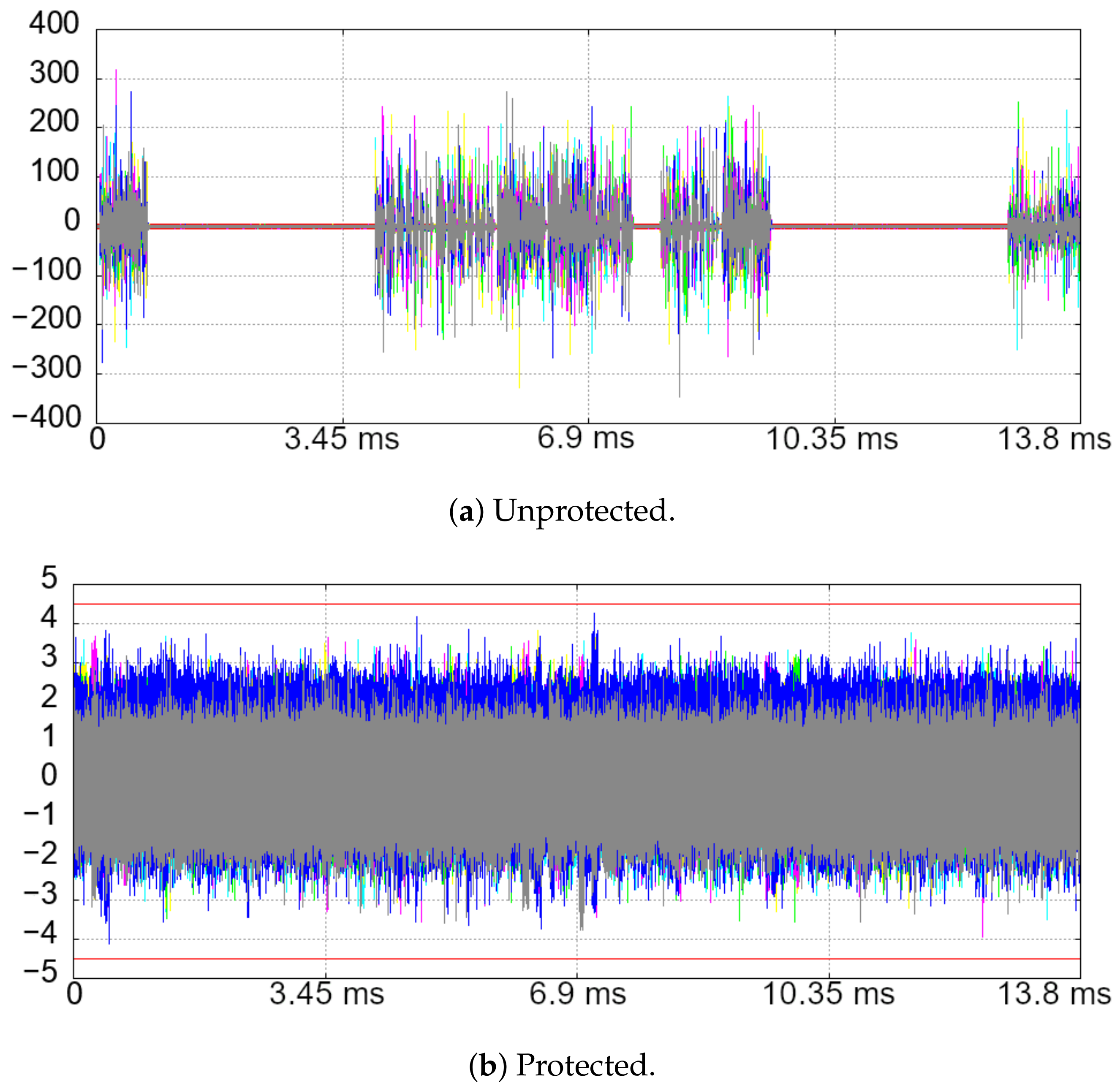
5.1. Side-Channel Leakage Evaluation

We describe our key-vs.-key t-test methodology in Section 5.1.1, and then, we present our results in Section 5.1.2. We used an attack-independent test vector leakage assessment methodology [35]. We were not able to detect any statistically significant leakage from the protected implementation.

5.1.1. Methodology

We implemented Rainbow with the proposed equivalent key scheme (using the unprotected reference implementation) on a 32-bit STM32F303 microcontroller based on the ARM Cortex-M4 core. To allow for a thorough and feasible side-channel evaluation of the proposed countermeasure, we chose Rainbow parameters ${\mathbb{F}}_q=GF\left(16\right),v_1=o_1=o_2=8$ to shorten the signing algorithm runtime compared to the Ia or Vc variants. We used the proposed efficient implementation of the equivalent keys scheme. The microcontroller was mounted in a ChipWhisperer C308 stand-alone evaluation board powered by an external 5 V laboratory power supply and clocked by a 7.37 MHz crystal.

The embedded Rainbow implementation receives a random seed from a controlling PC, which is then expanded using a linear congruential generator. The microcontroller then performs multiple signings without any external communication. Based on the generated pseudorandom numbers, the implementation generates the digests to be signed and also chooses one of four predefined private keys. This way, the microcontroller signs multiple randomly generated digests, each one using one of four randomly chosen private keys. The randomly interleaved private keys are a necessary prerequisite for our leakage evaluation methodology, as described later. When the signings are done, the microcontroller sends a checksum of the signatures back to the controlling PC, and the whole process is repeated as many times as necessary. This approach allows for a significant speedup of the measurement process.

Voltage drops over the core were amplified using the Langer EMV-Technik PA303 preamplifier and sampled using the Picoscope 6404D oscilloscope. A $10\Omega$ shunt resistor was used. The oscilloscope had a 25 MHz bandwidth limiter enabled, and the measurement channel was set in DC 50 $\Omega$ mode (since the preamplifier acts like a DC blocker). The sampling rate was 312 MS/s, in our case resulting in over 4 million samples per trace. The measured traces were then decimated 1:10 to 31.2 MS/s to allow for a feasible evaluation while maintaining a good signal-to-noise ratio [36].

The voltage was sampled during each signing, which lasted approximately 13.8 ms. Each decimated power trace consisted of 430,560 samples. The unprotected and protected implementations were evaluated independently. For the unprotected implementation, one of the four original private keys was randomly chosen in every signing. For the protected implementation, an equivalent key of one of the four original private keys was randomly chosen, and the next equivalent key was generated from the previous one.

The side-channel leakage was then evaluated using a fixed-fixed t-test methodology [35]. The measured power traces were partitioned into four groups based on the original private key used during the signing. Welch’s t-statistic was then computed between every two groups (six evaluations in total), in every sampling point independently. The null hypothesis was that the two groups’ means are equal, i.e., the original keys are indistinguishable by the mean power consumption. The hypothesis was rejected for high values of the $\left|t\right|$-statistic according to the Student’s distribution and selected significance level. In side-channel leakage evaluation, the threshold of 4.5 or 5 is typically considered for the $\left|t\right|$-statistic, which must be further evaluated carefully with the possibility of both positive and negative false results in mind [35,37].

5.1.2. Results

Figure 1 depicts the results of the leakage evaluations. Figure 1a depicts the results of the evaluation on the unprotected implementation, where every t-test was performed using approximately 40,000 power traces. Figure 1b depicts the results for the protected implementation, where every t-test was performed using approximately one million power traces. Each graph contains six overlaid curves, one for each key-vs.-key t-test. As can be seen in Figure 1a, many peaks reach t-value of 200 and some even exceed 300, in contrast to Figure 1b, where the threshold of 4.5 (marked by red horizontal lines) is not surpassed by the protected implementation. Therefore, we did not detect any statistically significant side-channel leakage from our protected implementation during the signing.

5.2. Time Evaluation

We evaluated the time performance on three different platforms:

• The STM32F303 ARM microcontroller (a single-core Cortex-M4);
• A Raspberry Pi 3 B+ single-board computer equipped with the Broadcom BCM2837 ARM microprocessor (a four-core Cortex-A53);
• A desktop computer equipped with an Intel Core i5-2400 processor (four cores).

On the STM32F303 microcontroller, we used the same parameters as for the leakage assessment, i.e., $v_1=o_1=o_2=8$, where the secret key size is 1776 bytes. On the Raspberry Pi and desktop computer, we used the parameters $v_1=o_1=o_2=32$, where the secret key size is 95,520 bytes. The Rainbow algorithm runtime was measured including random number generating using a linear congruent generator, excluding hashing. All the implementations were compiled with GCC without any optimizations enabled.

On the STM32F303 microcontroller, the time to sign a document was $13.8\mathrm{ms}$, and the average time to generate the equivalent key was $33.28\mathrm{ms}$. The whole signing including the equivalent key generation was $3.41$-times slower compared to the unsecured signing.

On the Raspberry Pi 3 single-board computer, the average time to sign a document was $7.72\mathrm{ms}$, and the average time to generate the equivalent key was $19.87\mathrm{ms}$. The whole signing including the equivalent key generation was $3.57$-times slower compared to the unsecured signing.

On the desktop computer, the average time to sign a document was $116\mathsf{\mu }\mathrm{s}$, and the average time to generate the equivalent key was $420\mathsf{\mu }\mathrm{s}$. The whole signing including the equivalent key generation was $4.62$-times slower compared to the unsecured signing.

For comparison, the randomization countermeasure of Rainbow proposed in [29] resulted in $3.31$-times slower signing.

Table 2. Time overhead comparison.

Implementation	Unprotected	Protected	Slowdown
Our countermeasure (STM32F303)	$13.8\mathrm{ms}$	$13.8+33.28=47.08\mathrm{ms}$1	$3.41\times$
Our countermeasure (RPi)	$7.72\mathrm{ms}$	$7.72+19.87=27.59\mathrm{ms}$1	$3.57\times$
Our countermeasure (PC)	$116\mathsf{\mu }\mathrm{s}$	$116+420=536\mathsf{\mu }\mathrm{s}$1	$4.62\times$
Countermeasure from [29]	$162,821$ cycles	$539,338$ cycles	$3.31\times$

¹ Our equivalent key can be precomputed any time prior to the signing, and then, the signing itself has no overhead.

summarizes the time overhead comparison. However, our equivalent key can be precomputed any time prior to the signing, and then, the signing itself has no overhead.

Figure 2 shows the calculation time of the individual generation components. Det is the time of the $(\mathbf{A},\mathbf{B})$ tuple generation including the regularity verification. ${\mathtt{T}}^{-1}\circ \mathtt{B}$, $\mathtt{A}\circ {\mathtt{S}}^{-1}$ and $\mathtt{A}\circ \mathtt{F}$ correspond to the calculation of ${\mathbf{T}}^{-1}\mathbf{B}$, ${\mathbf{AS}}^{-1}$, and $A\circ F$, respectively. The time of F∘B diag refers to Algorithm 1, and F∘B norm refers to Equation (48). The time of the signing itself is also included for comparison.

5.3. Memory Evaluation

From the memory perspective, the generating of the equivalent key is not an in-place algorithm due to the matrix multiplication in Equation (47). As the key structure is the same as for the unprotected version, we further describe only the extra variables needed for the generation of the equivalent key. The generating of the equivalent key does not need a dynamically allocated memory (as we assumed predefined parameters), and the biggest heap variable is the $(\mathbf{A},\mathbf{B})$ two-tuple itself, which only takes $(n+m)·{\log }_2\left(q\right)$ bits, where ${\log }_2\left(q\right)$ is the size of an element of ${\mathbb{F}}_q$ in bits. Other local variables are negligible. Additionally, one can split each part of the mask to be applied separately. This can further reduce extra memory needs to $\max (n,m)·{\log }_2\left(q\right)$ bits.

The implementation submitted to NIST uses a special case of the secret key, where matrices $\mathbf{S}$ and $\mathbf{T}$ are specifically selected for memory effectiveness. After the generating of the equivalent key, this special format is no longer possible. As a consequence, we obtained a slightly larger secret key, where the size difference was $(v_1^2+2o_1^2+2o_2^2)·{\log }_2\left(q\right)$ bits. For the Ia parameters, the difference was 2560 bytes, resulting in a key that was approximately $2.6\%$ larger. Our countermeasure also requires a minor modification of the submitted implementation.

Fresh random bits are needed during the generation and even during the signing process. The amount of randomness is deterministic, except the case where singular matrices are generated and need to be generated again. For the equivalent key generation, the mode (most common value) of the required bits of randomness is $(n+m)·{\log }_2\left(q\right)$, and for the signing process, it is $v_1·{\log }_2\left(q\right)$ (excluding the hashing salt). The mode is also a minimum number of required bits.

6. Conclusions

In this paper, we proposed a side-channel countermeasure for multivariate quadratic signature schemes. We used the Rainbow signature scheme as our use case. However, the proposed countermeasure is applicable to other schemes such as unbalanced oil and vinegar as well (UOV is equivalent to a single-layer Rainbow). We described the Rainbow algorithm and the notation used.

We proposed an equivalent private key scheme, in which a precomputed randomly generated equivalent key is used for signing instead of the original fixed private key. We examined the scheme in general and described its restrictions and security properties from the theoretical point of view. These include the number of different equivalent keys or reached entropy. We showed that the number of equivalent keys is enormous, and given that, we believe the probability of using the same equivalent key twice is negligible in practice. This efficiently prevents the attacker from mounting attacks such as differential or correlation power analysis.

We further proposed an efficient equivalent key scheme. Our scheme requires significantly less fresh randomness (bounded by the $O\left(n\right)$) than the general equivalent key (bounded by the $O\left(n^2\right)$) and allows for faster and more efficient computation. We described its properties, similar to the general case. We described an efficient algorithm for the generation of the equivalent key.

We evaluated our proposed countermeasure using attack-independent side-channel leakage assessment with one million power traces, and we were not able to detect any statistically significant information leakage. Lastly, we described the time and memory requirements of the countermeasure. The overhead of our countermeasure is comparable to other relevant countermeasures. Moreover, our equivalent key can be precomputed any time prior to the signing, and then, there is no overhead at the time of signing.

References

1. Meneghello, F.; Calore, M.; Zucchetto, D.; Polese, M.; Zanella, A. IoT: Internet of threats? A survey of practical security vulnerabilities in real IoT devices. IEEE Internet Things J. 2019, 6, 8182–8201. [Google Scholar] [CrossRef]
2. Daemen, J.; Rijmen, V. The Design of Rijndael; Springer: Berlin/Heidelberg, Germany, 2002; Volume 2. [Google Scholar]
3. Rivest, R.L.; Shamir, A.; Adleman, L. A method for obtaining digital signatures and public-key cryptosystems. Commun. ACM 1978, 21, 120–126. [Google Scholar] [CrossRef] [Green Version]
4. Koblitz, N. Elliptic curve cryptosystems. Math. Comput. 1987, 48, 203–209. [Google Scholar] [CrossRef]
5. Shor, P.W. Polynomial-time algorithms for prime factorization and discrete logarithms on a quantum computer. SIAM Rev. 1999, 41, 303–332. [Google Scholar] [CrossRef]
6. Ducas, L.; Kiltz, E.; Lepoint, T.; Lyubashevsky, V.; Schwabe, P.; Seiler, G.; Stehlé, D. CRYSTALS-Dilithium: Algorithm Specifications and Supporting Documentation. Available online: https://pq-crystals.org/ (accessed on 27 September 2022).
7. Fouque, P.A.; Hoffstein, J.; Kirchner, P.; Lyubashevsky, V.; Pornin, T.; Prest, T.; Ricosset, T.; Seiler, G.; Whyte, W.; Zhang, Z. Falcon: Fast-Fourier Lattice-Based Compact Signatures over NTRU. NIST PQC Project Round 2, Documentation. Available online: https://falcon-sign.info/ (accessed on 27 September 2022).
8. Ding, J.; Schmidt, D. Rainbow, a new multivariable polynomial signature scheme. In Proceedings of the International Conference on Applied Cryptography and Network Security, New York, NY, USA, 7–10 June 2005; Springer: Berlin/Heidelberg, Germany, 2005; pp. 164–175. [Google Scholar]
9. Kipnis, A.; Patarin, J.; Goubin, L. Unbalanced oil and vinegar signature schemes. In Proceedings of the International Conference on the Theory and Applications of Cryptographic Techniques, Prague, Czech Republic, 2–6 May 1999; Springer: Berlin/Heidelberg, Germany, 1999; pp. 206–222. [Google Scholar]
10. Beullens, W.; Preneel, B. Field lifting for smaller UOV public keys. In Proceedings of the International Conference on Cryptology in India, Chennai, India, 10–13 December 2017; Springer: Cham, Switzerland, 2017; pp. 227–246. [Google Scholar]
11. Kocher, P.; Jaffe, J.; Jun, B. Differential Power Analysis. In Advances in Cryptology — CRYPTO’ 99; Springer: Berlin/Heidelberg, Germany, 1999; pp. 388–397. [Google Scholar] [CrossRef] [Green Version]
12. Boer, B.d.; Lemke, K.; Wicke, G. A DPA attack against the modular reduction within a CRT implementation of RSA. In Proceedings of the International Workshop on Cryptographic Hardware and Embedded Systems, Redwood Shores, CA, USA, 13–15 August 2002; Springer: Berlin/Heidelberg, Germany, 2002; pp. 228–243. [Google Scholar]
13. Brier, E.; Clavier, C.; Olivier, F. Correlation Power Analysis with a Leakage Model. In Lecture Notes in Computer Science; Springer: Berlin/Heidelberg, Germany, 2004; pp. 16–29. [Google Scholar] [CrossRef] [Green Version]
14. Quisquater, J.J.; Samyde, D. Electromagnetic analysis (ema): Measures and counter-measures for smart cards. In Proceedings of the International Conference on Research in Smart Cards, Cannes, France, 19–21 September 2001; Springer: Berlin/Heidelberg, Germany, 2001; pp. 200–210. [Google Scholar]
15. Chari, S.; Rao, J.R.; Rohatgi, P. Template attacks. In Proceedings of the International Workshop on Cryptographic Hardware and Embedded Systems, Redwood Shores, CA, USA, 13–15 August 2002; Springer: Berlin/Heidelberg, Germany, 2002; pp. 13–28. [Google Scholar]
16. Rechberger, C.; Oswald, E. Practical template attacks. In Proceedings of the International Workshop on Information Security Applications, Jeju Island, Korea, 23–25 August 2004; Springer: Berlin/Heidelberg, Germany, 2004; pp. 440–456. [Google Scholar]
17. Lerman, L.; Poussier, R.; Markowitch, O.; Standaert, F.X. Template attacks versus machine learning revisited and the curse of dimensionality in side-channel analysis: Extended version. J. Cryptogr. Eng. 2018, 8, 301–313. [Google Scholar] [CrossRef]
18. Hettwer, B.; Gehrer, S.; Güneysu, T. Applications of machine learning techniques in side-channel attacks: A survey. J. Cryptogr. Eng. 2020, 10, 135–162. [Google Scholar] [CrossRef]
19. Timon, B. Non-profiled deep learning-based side-channel attacks with sensitivity analysis. IACR Trans. Cryptogr. Hardw. Embed. Syst. 2019, 2019, 107–131. [Google Scholar] [CrossRef]
20. Park, A.; Shim, K.A.; Koo, N.; Han, D.G. Side-Channel Attacks on Post-Quantum Signature Schemes based on Multivariate Quadratic Equations. IACR Trans. Cryptogr. Hardw. Embed. Syst. 2018, 2018, 500–523. [Google Scholar] [CrossRef]
21. Pokorný, D.; Socha, P.; Novotný, M. Side-channel attack on Rainbow post-quantum signature. In Proceedings of the 2021 Design, Automation Test in Europe Conference Exhibition (DATE), Grenoble, France, 1–5 February 2021; pp. 565–568. [Google Scholar] [CrossRef]
22. Tiri, K.; Verbauwhede, I. A logic level design methodology for a secure DPA resistant ASIC or FPGA implementation. In Proceedings of the Proceedings Design, Automation and Test in Europe Conference and Exhibition, Paris, France, 16–20 February 2004; Volume 1, pp. 246–251. [Google Scholar]
23. Popp, T.; Mangard, S. Masked dual-rail pre-charge logic: DPA-resistance without routing constraints. In Proceedings of the International Workshop on Cryptographic Hardware and Embedded Systems, Edinburgh, UK, 29 August–1 September 2005; Springer: Berlin/Heidelberg, Germany, 2005; pp. 172–186. [Google Scholar]
24. Lu, Y.; O’Neill, M.; McCanny, J. Evaluation of random delay insertion against DPA on FPGAs. ACM Trans. Reconfigurable Technol. Syst. (TRETS) 2010, 4, 1–20. [Google Scholar] [CrossRef]
25. Baddam, K.; Zwolinski, M. Evaluation of dynamic voltage and frequency scaling as a differential power analysis countermeasure. In Proceedings of the 20th International Conference on VLSI Design held jointly with 6th International Conference on Embedded Systems (VLSID’07), Bangalore, India, 6–10 January 2007; pp. 854–862. [Google Scholar]
26. Nikova, S.; Rechberger, C.; Rijmen, V. Threshold implementations against side-channel attacks and glitches. In Proceedings of the International Conference on Information and Communications Security, Raleigh, NC, USA, 4–7 December 2006; Springer: Berlin/Heidelberg, Germany, 2006; pp. 529–545. [Google Scholar]
27. Bilgin, B.; Gierlichs, B.; Nikova, S.; Nikov, V.; Rijmen, V. Higher-order threshold implementations. In Proceedings of the International Conference on the Theory and Application of Cryptology and Information Security, Kaoshiung, Taiwan, 7–11 December 2014; Springer: Berlin/Heidelberg, Germany, 2014; pp. 326–343. [Google Scholar]
28. Gross, H.; Mangard, S.; Korak, T. Domain-Oriented Masking: Compact Masked Hardware Implementations with Arbitrary Protection Order. In Proceedings of the 2016 ACM Workshop on Theory of Implementation Security, Vienna, Austria, 24 October 2016; p. 3. [Google Scholar]
29. Shim, K.A.; Park, C.M.; Baek, Y.J. Lite-Rainbow: Lightweight Signature Schemes Based on Multivariate Quadratic Equations and Their Secure Implementations. In Proceedings of the Progress in Cryptology–INDOCRYPT 2015; Biryukov, A., Goyal, V., Eds.; Springer International Publishing: Cham, Switzerland, 2015; pp. 45–63. [Google Scholar]
30. Beullens, W. Breaking Rainbow Takes a Weekend on a Laptop. Cryptology ePrint Archive, Report 2022/214. 2022. Available online: https://ia.cr/2022/214 (accessed on 27 September 2022).
31. Wolf, C.; Preneel, B. Equivalent keys in Multivariate Quadratic public key systems. J. Math. Cryptol. 2011, 4, 375–415. [Google Scholar] [CrossRef]
32. PQCRainbow.org. Available online: https://www.pqcrainbow.org/ (accessed on 27 September 2022).
33. Andrews, G.E.; Berndt, B. Ramanujan’s Lost Notebook; Springer: New York, NY, USA, 2005. [Google Scholar] [CrossRef]
34. Suprunenko, D.; Hirsch, K.; Society, A.M. Matrix Groups; Translations of Mathematical Monographs; American Mathematical Society: Providence, RI, USA, 1976. [Google Scholar]
35. Schneider, T.; Moradi, A. Leakage assessment methodology. J. Cryptogr. Eng. 2016, 6, 85–99. [Google Scholar] [CrossRef]
36. O’Flynn, C.; Chen, Z. Synchronous sampling and clock recovery of internal oscillators for side-channel analysis and fault injection. J. Cryptogr. Eng. 2015, 5, 53–69. [Google Scholar] [CrossRef]
37. Standaert, F.X. How (not) to use welch’s t-test in side-channel security evaluations. In Proceedings of the International Conference on Smart Card Research and Advanced Applications, Montpellier, France, 12–14 November 2018; Springer: Cham, Switzerland, 2018; pp. 65–79. [Google Scholar]
Figure 1. Results of the t-tests. Each graph contains six overlaid curves. The t-value is depicted on the vertical axis, and time is on the horizontal axis.
Electronics 11 03607 g001
Figure 2. Execution times of the components in equivalent key generation.
Electronics 11 03607 g002