Abstract
In this paper, a novel method termed the cosine approach is proposed to address the sidelobe suppression problem in MIMO radar transmit beampattern matching design. In contrast to the traditional optimization algorithms that try to find the optimum solutions from feasible regions, the proposed method, starting from outside the feasible regions, aims to obtain a satisfactory solution from a series of optimal transmit beampatterns. We first standardized the sidelobe suppression problem in MIMO radar transmit beampattern matching design and put forward four criteria to guide the micro-adjustment to the desired beampattern. Then, the cosine method was proposed to adjust the desired beampattern as well as increase the main-to-sidelobe ratio (MSLR) of the transmit beampattern. Finally, several numerical examples were chosen to test the effectiveness and advantages of the proposed method.
1. Introduction
In attempts to solve the MIMO radar transmit beampattern matching design problem, many optimal algorithms have been developed to obtain transmit signals [1,2,3,4,5,6,7,8,9,10,11,12,13,14,15,16,17,18,19,20,21,22,23,24,25,26,27,28,29,30,31,32,33], such as the gradient search algorithms [1,2], semi-definite programming algorithm [3,4,14,20], convex optimization techniques [5,23], cyclic minimization algorithm [6,7,9,10,11], and transmit beamspace processing techniques [8,12,13]. Although all these methods provide a comparatively good match to the desired beampattern, high sidelobes may still appear because the number of element positions is limited, or the desired beampattern cannot be expanded with finite Fourier series. Thus, it has become a challenge to design transmit signals to satisfy the constraint of the main-to-sidelobe ratio (i.e., the ratio of the maximum peak values of main lobe to sidelobe) as well as to match the desired beampattern as perfectly as possible.
Recently, several methods have been put forward to address the sidelobe suppression problem [29,34,35,36,37,38,39], in which various optimal models are established with the objective of reducing sidelobe peaks. In contrast with these optimal models, sidelobe suppression in transmit beampattern matching designs aims to minimize the errors between the desired and the transmit beampatterns, while accepting the constraint of the sidelobe. Thus far, there has been little discussion of this issue in the literature. Li and Stocia [3] provided a weighted optimization model to reduce the sidelobe peak in a MIMO radar transmit beampattern matching design; Hua and Abeysekera [22] developed another weighted optimization model to control the ripple levels within the energy focusing section and the transition bandwidth. However, in these approaches it is difficult to determine the weights, making it hard to balance the sidelobe suppression and the error between the desired and the transmit beampatterns.
In this paper, we propose a novel method termed the cosine method to address the sidelobe suppression problem in MIMO radar transmit beampattern matching design. Through matching the continually micro-adjusted desired beampattern, the final transmit beampattern can not only provide relatively good matching to the original desired beampattern but also has higher MSLR. In contrast to the traditional optimization algorithms which try to find the optimum solutions from feasible regions, the proposed cosine method, starting from the outside of a feasible region, obtains a satisfactory solution from a series of optimal transmit beampatterns.
This paper is organized as follows: Section 2 introduces the sidelobe suppression problem in transmit beampattern matching design, and establishes a sidelobe suppression model; Section 3 discusses the cosine method in detail, including its theoretical analysis and algorithm; Section 4 provides several examples to test the practicability and efficiency of the proposed method and conclusions are drawn in Section 5.
The notations in this paper are standard: represents the transpose of a matrix or vector, is the conjugate transpose of a matrix or vector, denotes the statistical expectation, and means the Euclidean norm of a vector.
2. Sidelobe Suppression Model
Consider an M-element uniform linear array (ULA) with inter-element spacing in a MIMO radar system and targets at the far field of the array. The transmit signals are defined as
where means the mth transmit signal with the power equal to 1. The beampattern of can be written as
where the steering vector is given by
where denotes the azimuth angle and . The correlation matrix of can be written as
where satisfies
The sidelobe suppression problem in MIMO radar transmit beampattern matching design can be expressed as follows:
On condition of fixed transmit element positions and constant transmit energy for each element, and given a desired beampattern and sidelobe constraint (MSLR > dB), how can we produce the transmit signal , making the transmit beampattern generated by match the desired beampattern as closely as possible? We may standardize this sidelobe suppression problem using the following model:
3. Cosine Method for Sidelobe Suppression
For Model (I), due to the main lobe broadening in the solving process, it is often difficult to identify its feasible region. In this section, we propose a novel method, namely the cosine method, to obtain a satisfactory solution. The iterative method includes 3 steps:
- Step 1:
- Make the micro-adjustment to the desired beampattern to obtain a new desired beampattern;
- Step 2:
- Provide a minimum mean square error matching the new desired beampattern and obtain an optimal transmit beampattern;
- Step 3:
- Calculate the MSLR of the transmit beampattern. If it is not meet the MSLR constraint, go back to Step 1.
Indeed, since [27] has provided a minimum mean square approximation of the desired beampattern, our cosine method focuses on how to make the micro-adjustment to the desired beampattern. In the following sections, we will explain how to achieve this adjustment.
3.1. Criteria for Micro-Adjustment to the Desired Beampattern
The purpose of continual micro-adjustments to the desired beampattern is to ensure the final transmit beampattern not only has a relatively good match to the original desired beampattern, but also a higher MSLR. Therefore, the slightly adjusted desired beampattern should not only meet the basic requirements of the desired beampattern [27], but also meet the basic properties of the transmit beampattern. To guide these adjustments, we provide the following four criteria:
- ;
- ;
- should be continuous and exists first order derivative;
- .
Where is micro-adjustments to the desired beampattern . The criteria 1–2 derive from the basic requirements of the desired beampattern [27]; criteria 3 derives from the transmit beampattern that can be expanded with finite Fourier series; as M increases, the mean square error between transmit beampattern and will tend to zero, so we have criteria 4. In order to obtain a good matching transmit beampattern with higher MSLR, all four criteria are necessary for the micro-adjustment to the desired beampattern.
According to the above four criteria, we may find many approaches to adjust the desired beampattern. Among them, Fourier expansion is often used as an approximation to a function. Let the Fourier expansion of the desired beampattern be
Then the sum of the first M items is
For , we have the following conclusion:
Lemma 1.
[40]: Let be the sum of the first M items of the Fourier expansions for the desired beampattern , and be the arbitrary M-1 trigonometric polynomial, i.e.,
then we have
where
Lemma 1 shows that is the minimum mean square approximation to in all M-1 trigonometric polynomial. It is obvious that satisfies criteria 2–4. However, according to [27], the desired beampattern and its finite Fourier expansion have the same optimal transmit beampattern . Therefore, if cannot satisfy the MSLR constraint, we need to explore other approach to increase MSLR as well as meet the four criteria.
3.2. Cosine Method
In this study, a novel method termed the cosine method is proposed to make the micro-adjustment to the desired beampattern.
First, we identify the largest bias point between the transmit beampattern and the desired beampattern , i.e.,
where is the minimum mean square matching design of [27].
Then, we select the maximum monotone interval within satisfying
Finally, we use in to replace the corresponding part of as follows:
(a) In the case of , we use in to replace the corresponding part of the desired beampattern . Then the adjusted desired beampattern is
(b) In the case of , we may adjust the desired beampattern in the strict monotone intervals and . in and is used to replace the corresponding parts of the desired beampattern . Then, the adjusted desired beampattern is
(c) In the case of , we may adjust the desired beampattern in the strict monotone intervals and . Similar to (b), the adjusted desired beampattern is
3.3. Four Criteria Examination
For the in Equations (10)–(12), we may use stretch transformation to change
Considering , it is obvious that , satisfying criterion 1.
From Equation (13), we have . Thus also meets criterion 2.
Consider
We have the following conclusions:
Lemma 2.
For a sufficiently large M, if is a strict monotone interval of , thenis also the monotone interval of.
From Lemma 2, since
satisfies criterion 3.
Theorem 3.
If the desired beampattern is a continuous function and is obtained from Equations (10)–(12), then
Proof:
Here, we only provide the proof in the case of . The other cases are similar to this case. Since
for when , we have
By Equations (10) and (13)
that is,
From Theorem 3, we know that satisfies criterion 4. □
3.4. Algorithm
According to the theoretical analysis above, given the sidelobe suppression level , here we provide an algorithm to explain our proposed cosine method:
- Step 1:
- Let i = 0, ;
- Step 2:
- Use the one-step approach in [27] to obtain the transmit beampattern with minimum mean square error to the desired beampattern ;
- Step 3:
- If , then go to end; otherwise, go to Step 4;
- Step 4:
- Solve , satisfyingand let be the first M items of Fourier expansion, identify the strict monopoly area with in .
- Step 5:
- If , use Equation (10) to obtain ;If , use Equation (11) to obtain ;If , use Equation (12) to obtain ;
- Step 6:
- Implement stretch transformation to , let
- Step 7:
- Let i = i + 1, return to Step 2.
Note: If the desired beampattern is a symmetric figure, we may simultaneously adjust in the strict monopoly areas and for .
4. Numerical Examples
Example 1.
Consider the following standardized symmetric triangle desired beampattern [4,29,34].
Here, , .
Figure 1 shows the optimal matching transmit beampattern with the first sidelobe peak, 2.6285. The MSLR = 12.334 dB is lower than the sidelobe suppression level (16 dB), thereby not satisfying the sidelobe constraint. Hence, the cosine approach is employed to increase MSLR. As shown in Figure 1, since the bias between and reaches the maximum at , the monotone intervals and containing are chosen to adjust the desired beampattern .
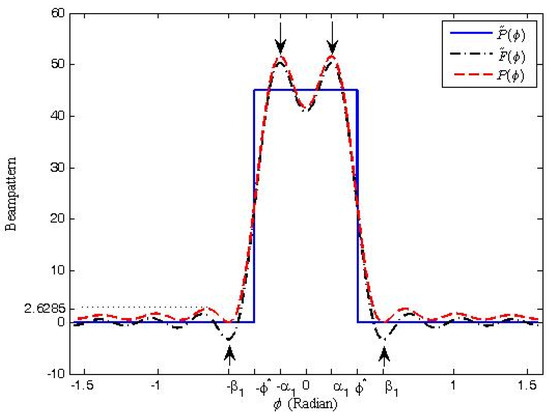
Figure 1.
Optimal transmit beampattern vs. desired beampattern (M = 10).
Figure 2 illustrates the optimal matching beampatterns after using the cosine method, where represents using the cosine method 1, 2, 3 times, respectively. As we can see, the first sidelobe peak of is 1.0912 with MSLR = 16.152 dB, satisfying the sidelobe constraint. Table 1 provides the results after using the cosine method each time.
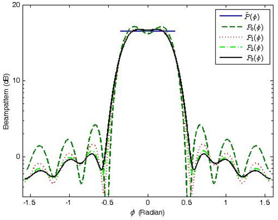
Figure 2.
The transmit beampatterns after using the cosine method 1–3 times (M = 10).

Table 1.
Results of the cosine method for Example 1.
As shown in Table 1, the sidelobe peaks of the transmit beampatterns are decreasing while their MSLR are increasing. After three adjustments, the MSLR increases 30.96% with only a 20.67% increase of the mean square error between the transmit beampattern and the original desired beampattern . Thus, is a satisfactory solution of Example 1. As illustrated in Figure 2, the proposed cosine method can not only increase the MSLR significantly but also provide a comparatively good match to the desire beampattern.
Compared with [34], our cosine method can obtain a lower MSLR. For M = 16, Figure 3 illustrates the optimal matching beampatterns after using the cosine method, where represents using the cosine method 1, 5, and 10 times, respectively. After ten adjustments, the MSLR increased from 10.123 dB to 18.125 dB. Compared with [29], our cosine method also obtained a lower MSLR.
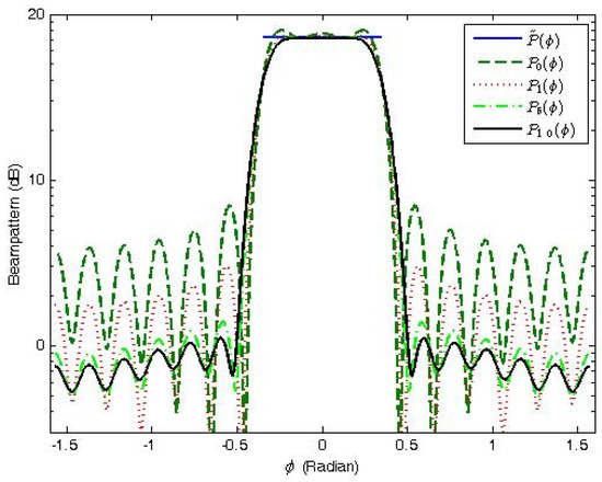
Figure 3.
The transmit beampatterns after using the cosine method (M = 16).
Example 2.
Consider an asymmetric desired beampattern.
Here, .
Figure 4 illustrates the comparisons between the transmit beampattern and the transmit beampattern using the cosine method 7 times. For the , the MSLR is 9.7842 dB, lower than the sidelobe suppression level . However, after using the cosine method 7 times, the MSLR increased 43.24%, reaching 14.0183 dB, while the mean square error to the desired beampattern only increased 19.05% to 14.4256, showing the advantage of the cosine method for suppressing sidelobes in the beampattern matching design problem.
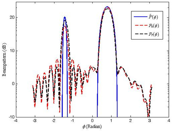
Figure 4.
The desired beampattern vs. the transmit beampattern obtained using the cosine method 7 times (M = 20).
Example 3.
Consider a desired beampattern with a nonuniform linear array:
Here, and . The positions of the elements are .
Figure 5 compares and the transmit beampattern . The MSLR of is 9.7754 dB, much lower than . After 20 times adjustments by the cosine approach, the MSLR reached 11.0002 dB, satisfying the sidelobe suppression level . Compared to the 12.53% increase in the MSLR, the mean square error between and only increased 1.26%, reaching 16.584.
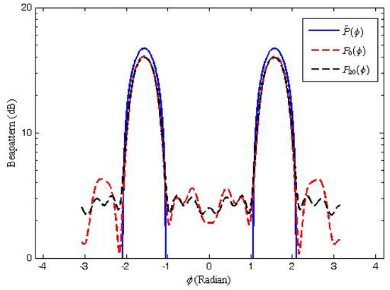
Figure 5.
The desired beampattern vs. the transmit beampattern obtained by using the cosine method 20 times (M = 10).
From Examples 1–3, we may find that the proposed cosine method can not only significantly increase the MSLR, but also provide very good matching to the desired beampattern. In addition, this cosine method is suitable for both symmetric and asymmetric arrays. Therefore, the cosine method is an effective and efficient solution to the problem of sidelobe suppression in beampattern matching design.
5. Conclusions
In this paper, a novel method, the cosine method, is proposed for addressing the problem of sidelobe suppression in beampattern matching design, in which the MSLR is a constraint. The theoretical justification and algorithm for this method were provided and several numerical examples were tested to examine the advantages of the proposed method. Indeed, the cosine method showed significant improvement in MSLR but also increased the mean square error between the desired and transmit beampatterns. However, considering the trade-off between sidelobe level and total bias, the proposed method produces a substantial increase in the MSLR at the expense of a relatively small increase of the mean square error. In real application, we may combine this cosine method with more radar transmit arrays to increase the sidelobe suppression level as well as to obtain better matching beampattern.
Author Contributions
X.Z. conceived the article’s idea and was responsible for drafting the manuscript to the final stage. Z.H. was involved in the article structure. The authors declare no competing interests. All authors have read and agreed to the published version of the manuscript.
Funding
This research was funded by the National Natural Science Foundation of China (No. 61771004).
Data Availability Statement
All data used in this article are available in the main text.
Acknowledgments
We would like to thank Lez Rayman Bacchus for the language editing of the final version.
Conflicts of Interest
The authors declare no conflict of interest.
References
- Fuhrmann, D.R.; Antonio, G.S. Transmit beamforming for MIMO radar systems using partial signal correlation. In Proceedings of the Conference Record of the Thirty-Eighth Asilomar Conference on Signals, Systems and Computers, Pacific Grove, CA, USA, 1 November 2004; pp. 295–299. [Google Scholar]
- Aittomaki, T.; Koivunen, V. Signal covariance matrix optimization for transmit beamforming in MIMO radars. In Proceedings of the Conference Record of the Forty-First Asilomar Conference on Signals, Systems and Computers, Pacific Grove, CA, USA, 4–7 November 2007; pp. 182–186. [Google Scholar]
- Li, J.; Stoica, P. MIMO Radar with Colocated Antennas. IEEE Signal Process. Mag. 2007, 24, 106–114. [Google Scholar] [CrossRef]
- Stoica, P.; Li, J.; Xie, Y. On probing signal design for MIMO radar. IEEE Trans. Signal Process. 2007, 55, 4151–4161. [Google Scholar] [CrossRef]
- Fuhrmann, D.R.; Antonio, G.S. Transmit beamforming for MIMO radar systems using signal cross-correlation. IEEE Trans. Aerosp. Electron. Syst. 2008, 44, 171–186. [Google Scholar] [CrossRef]
- Stoica, P.; Li, J.; Zhu, X. Waveform synthesis for diversity-based transmit beampattern design. IEEE Trans. Signal Process. 2008, 56, 2593–2598. [Google Scholar] [CrossRef]
- Li, J.; Stoica, P.; Zheng, X. Signal Synthesis and Receiver Design for MIMO Radar Imaging. IEEE Trans. Signal Process. 2008, 56, 3959–3968. [Google Scholar] [CrossRef]
- Hassanien, A.; Vorobyov, S.A. Direction finding for MIMO radar with colocated antennas using transmit beamspace processing. In Proceedings of the 3rd IEEE International Workshop on Computational Advances in Multi-Sensor Adaptive Processing (CAMSAP), Aruba, Netherland Antilles, 13–16 December 2009; IEEE: Piscataway, NJ, USA, 2009; pp. 181–184. [Google Scholar]
- He, H.; Stoica, P.; Li, J. Designing Unimodular Sequence Sets With Good Correlations—Including an Application to MIMO Radar. IEEE Trans. Signal Process. 2009, 57, 4391–4405. [Google Scholar] [CrossRef]
- Roberts, W.; He, H.; Li, J.; Stoica, P. Probing Waveform Synthesis and Receiver Filter Design. IEEE Signal Process. Mag. 2010, 27, 99–112. [Google Scholar] [CrossRef]
- He, H.; Stoica, P.; Li, J. Wideband MIMO Systems: Signal Design for Transmit Beampattern Synthesis. IEEE Trans. Signal Process. 2010, 59, 618–628. [Google Scholar] [CrossRef]
- Khabbazibasmenj, A.; Hassanien, A.; Vorobyov, S.A. Transmit beamspace design for direction finding in colocated MIMO radar with arbitrary receive array. In Proceedings of the IEEE International Conference on Acoustics, Speech and Signal Processing (ICASSP), Prague, Czech Republic, 22–27 May 2011; pp. 2784–2787. [Google Scholar]
- Hassanien, A.; Vorobyov, S.A. Transmit Energy Focusing for DOA Estimation in MIMO Radar with Colocated Antennas. IEEE Trans. Signal Process. 2011, 59, 2669–2682. [Google Scholar] [CrossRef]
- Naghibi, T.; Behnia, F. MIMO Radar Waveform Design in the Presence of Clutter. IEEE Trans. Aerosp. Electron. Syst. 2011, 47, 770–781. [Google Scholar] [CrossRef]
- Ahmed, S.; Thompson, J.S.; Petillot, Y.R.; Mulgrew, B. Unconstrained Synthesis of Covariance Matrix for MIMO Radar Transmit Beampattern. IEEE Trans. Signal Process. 2011, 59, 3837–3849. [Google Scholar] [CrossRef]
- Ahmed, S.; Thompson, J.S.; Petillot, Y.R.; Mulgrew, B. Finite alphabet constant-envelope waveform design for MIMO radar. IEEE Trans. Signal Process. 2011, 59, 5326–5337. [Google Scholar] [CrossRef]
- Friedlander, B. On Transmit Beamforming for MIMO Radar. IEEE Trans. Aerosp. Electron. Syst. 2012, 48, 3376–3388. [Google Scholar] [CrossRef]
- Wilcox, D.; Sellathurai, M. On MIMO Radar Subarrayed Transmit Beamforming. IEEE Trans. Signal Process. 2011, 60, 2076–2081. [Google Scholar] [CrossRef]
- Wang, Y.-C.; Wang, X.; Liu, H.; Luo, Z.-Q. On the Design of Constant Modulus Probing Signals for MIMO Radar. IEEE Trans. Signal Process. 2012, 60, 4432–4438. [Google Scholar] [CrossRef]
- Hua, G.; Abeysekera, S.S. Colocated MIMO radar transmit beamforming using orthogonal waveforms. In Proceedings of the IEEE International Conference on Acoustics, Speech and Signal Processing, Kyoto, Japan, 25–30 March 2012; pp. 2453–2456. [Google Scholar]
- Shadi, K.; Behnia, F. MIMO Radar Beamforming Using Orthogonal Decomposition of Correlation Matrix. Circuits Syst. Signal Process. 2013, 32, 1791–1809. [Google Scholar] [CrossRef]
- Hua, G.; Abeysekera, S.S. MIMO Radar Transmit Beampattern Design With Ripple and Transition Band Control. IEEE Trans. Signal Process. 2013, 61, 2963–2974. [Google Scholar] [CrossRef]
- Gong, P.; Shao, Z.; Tu, G.; Chen, Q. Transmit beampattern design based on convex optimization for MIMO radar systems. Signal Process. 2014, 94, 195–201. [Google Scholar] [CrossRef]
- Lipor, J.; Ahmed, S.; Alouini, M.-S. Fourier-Based Transmit Beampattern Design Using MIMO Radar. IEEE Trans. Signal Process. 2014, 62, 2226–2235. [Google Scholar] [CrossRef]
- Ahmed, S.; Alouini, M.-S. MIMO Radar Transmit Beampattern Design Without Synthesising the Covariance Matrix. IEEE Trans. Signal Process. 2014, 62, 2278–2289. [Google Scholar] [CrossRef]
- Khabbazibasmenj, A.; Hassanien, A.; Vorobyov, S.A.; Morency, M.W. Efficient Transmit Beamspace Design for Search-Free Based DOA Estimation in MIMO Radar. IEEE Trans. Signal Process. 2014, 62, 1490–1500. [Google Scholar] [CrossRef]
- Zhang, X.; He, Z.; Rayman-Bacchus, L.; Yan, J. MIMO Radar Transmit Beampattern Matching Design. IEEE Trans. Signal Process. 2015, 63, 2049–2056. [Google Scholar] [CrossRef]
- Cheng, Z.; He, Z.; Zhang, S.; Li, J. Constant Modulus Waveform Design for MIMO Radar Transmit Beampattern. IEEE Trans. Signal Process. 2017, 65, 4912–4923. [Google Scholar] [CrossRef]
- Fan, W.; Liang, J.; Li, J. Constant modulus MIMO radar waveform design with minimum peak sidelobe transmit beampattern. IEEE Trans. Signal Process. 2018, 66, 4207–4222. [Google Scholar] [CrossRef]
- Yu, X.; Cui, G.; Yang, J.; Kong, L.; Li, J. Wideband MIMO radar waveform design. IEEE Trans. Signal Process. 2019, 67, 3487–3501. [Google Scholar] [CrossRef]
- Cheng, Z.; Liao, B.; He, Z.; Li, J.; Xie, J. Joint Design of the Transmit and Receive Beamforming in MIMO Radar Systems. IEEE Trans. Veh. Technol. 2019, 68, 7919–7930. [Google Scholar] [CrossRef]
- Hong, S.; Dong, Y.; Xie, R.; Ai, Y.; Wang, Y. Constrained Transmit Beampattern Design Using a Correlated LFM-PC Waveform Set in MIMO Radar. Sensors 2020, 20, 773. [Google Scholar] [CrossRef] [PubMed]
- Yu, X.; Qiu, H.; Wei, J.Y.W.; Cui, G. Multi-spectrally constrained MIMO radar beampattern design via sequential convex approximation. IEEE Trans. Aerosp. Electron. Syst. 2022, 58, 2935–2949. [Google Scholar] [CrossRef]
- Shariati, N.; Zachariah, D.; Bengtsson, M. Minimum sidelobe beampattern design for MIMO radar systems: A robust approach. In Proceedings of the 2014 IEEE International Conference on Acoustics, Speech and Signal Processing (ICASSP), Florence, Italy, 4–9 May 2014; pp. 5312–5316. [Google Scholar]
- Ahmed, S.; Alouini, M.-S. MIMO-Radar Waveform Covariance Matrix for High SINR and Low Side-Lobe Levels. IEEE Trans. Signal Process. 2014, 62, 2056–2065. [Google Scholar] [CrossRef]
- Zhou, S.; Liu, H.; Wang, X.; Cao, Y. MIMO radar range-angular-doppler sidelobe suppression using random space-time coding. IEEE Trans. Aerosp. Electron. Syst. 2014, 50, 2047–2060. [Google Scholar] [CrossRef]
- Ma, C.; Yeo, T.S.; Tan, C.S.; Qiang, Y.; Zhang, T. Receiver Design for MIMO Radar Range Sidelobes Suppression. IEEE Trans. Signal Process. 2010, 58, 5469–5474. [Google Scholar] [CrossRef]
- Xu, H.; Blum, R.S.; Wang, J.; Yuan, J. Colocated MIMO radar waveform design for transmit beampattern formation. IEEE Trans. Aerosp. Electron. Syst. 2015, 51, 1558–1568. [Google Scholar] [CrossRef]
- Davis, M.S.; Lanterman, A.D. Minimum integrated sidelobe ratio filters for MIMO radar. IEEE Trans. Aerosp. Electron. Syst. 2015, 51, 405–416. [Google Scholar] [CrossRef]
- Boggess, A.; Narcowich, J. A First Course in Wavelets with Fourier Analysis, 2nd ed.; John Wiley & Sons, Inc.: Hoboken, NJ, USA, 2009. [Google Scholar]


Publisher’s Note: MDPI stays neutral with regard to jurisdictional claims in published maps and institutional affiliations. |
© 2022 by the authors. Licensee MDPI, Basel, Switzerland. This article is an open access article distributed under the terms and conditions of the Creative Commons Attribution (CC BY) license (https://creativecommons.org/licenses/by/4.0/).