Abstract
The detection of edges in images is a pressing issue in the field of image processing. This technique has found widespread application in image pattern recognition, machine vision, and a variety of other areas. The feasibility and effectiveness of grey theory in image engineering applications have prompted researchers to continuously explore it. The grey model (GM (1,1)) with the first-order differentiation of one variable is the grey prediction model that is most frequently used. It is a typical trend analysis model and can be used for image edge detection. The traditional integer-order differential image edge detection operator has problems such as blurred and discontinuous edges, incomplete image details, and high influence by noise. We present a novel grey model for detecting image edges based on a fractional-order discrete operator in this paper. To improve the features of the original image, our model first preprocesses it before calculating the prediction of the original image using our fractional-order cumulative greyscale model. We obtain the edge information of the image by first subtracting a preprocessed image from the predicted image and then eliminating isolated noise points using the median filtering method. Based on the discrete wavelet transform, image edges are finally extracted. The comparison experiments with a traditional edge detection operator show that our algorithm can accurately locate the image edges, the image edges are clear and complete, and this model has better anti-noise performance.
1. Introduction
Accurate image edge detection is crucial for image analysis and computation, making it one of the most challenging image processing techniques. The detection of image edges is the fundamental building block of image analysis and processing, and it holds a unique place in both the fields of image processing and computer vision. Image edge detection occupies a special place in the society of image processing and computer vision. In an image, edges are the pixels with rapidly changing greyscale [1], and the stronger the local greyscale change, the more it proves the existence of an edge at that location [2]. Edges depict the main image feature information and reflect the discontinuity of image local features, and thus they are very important for image analysis. There exist many image edge detection methods based on classical integer-order differential operators in the field of image processing, which are mainly based on pixel gradients [3], such as Roberts [4], Sobel [5], Prewitt [6], Laplacian [7], Canny [8], etc. Among these traditional edge detection operators, Roberts is better for processing low-noise images with steep grey change, but the extracted edges by it are often coarser and more sensitive to noise; the Sobel operator and the Prewitt operator are more effective for processing the images with gentle greyscale changes and much noise but are less effective for those with mixed multiple complex noises. Laplacian is precise in locating image step edge points, but it is highly sensitive to noise and prone to producing detection edges with discontinuities; Canny is not easily affected by noise and can detect the real weak edges, but it often loses the high-frequency edge information in its anti-noise process. Other image edge detection methods include fuzzy edge detection [9], neural network edge detection [10], and wavelet edge detection [11], among others. Fractional-order calculus is obtained by changing its order to a fraction based on integer-order calculus. The theory related to fractional-order calculus appeared after the concept of fractal doctrine was introduced. It was not until the 1980s, when B. Mandelbrot of Yale University applied the Riemann–Liouville fractional-order calculus to the Brownian motion of fractal media, that the fractional-order calculus gained rapid development and became a hot research topic at home and abroad, and was widely used in many fields. It is currently utilized in numerous fields. Image processing increasingly uses fractional-order calculus theory. The image edge extraction using traditional integer-order calculus extracts incomplete detail information, while fractional-order calculus has unique advantages in processing images with complex texture structures, which can retain more texture details. Therefore, fractional-order calculus theory is increasingly used in image processing. Based on the properties of fractional-order calculus, Pu et al. [12] derived several fractional differential-based image texture enhancement masks for image enhancement applications. Compared with the integer differentiation operator, this method can effectively enhance the edge information of the image and produce better enhancement effects. In [13], Tian et al. proposed a new fractional-order Laplacian for image edge detection, which utilizes the global characteristic of the fractional derivatives to extract more image edge details. J. E. Lavín-Delgado et al. [14] proposed a new fractional-order mask for the edge detection of images without singular kernels based on Caputo–Fabrizio fractional-order derivatives and applied it to edge detection of medical images. In [15], M. Hacini et al. proposed a two-dimensional fractional derivative mask for image feature edge detection, which can detect more details of the image. Wang et al. [16] applied wavelet soft thresholding denoising to the fractional-order derivative algorithm to detect image edges and obtained better signal-to-noise ratio and edge extraction results.
Grey system theory was originally proposed to deal with the problems in small data and bad information objects [17]. A sub-field of grey system theory is grey prediction theory. The grey prediction model’s benefit is that it can produce precise prediction results based on sparse data [18]. Currently, grey prediction models have been widely and successfully used in a variety of disciplines, including energy, economy, and engineering [19], with the GM(1,1) model being the most popular. Grey system theory has also been applied to image edge detection, and some good results have been achieved so far. Ma et al. [20] tried to use the grey system theory for edge detection in images by determining the reference sequence of non-edge points and the sequence to be compared and distinguishing edge points from non-edge points according to the grey correlation between the two sequences. He et al. [21] employed a four-point prediction model based on the GM (1,1) approach to detect image edges, which is a substantial contribution to the grey prediction model used for image edge identification. Li et al. discussed an edge detection method based on the GM (1,1) model, and it can detect image edges from eight directions and is applied to detect license plate edges for cars [22]. Xie et al. changed the exponent of the GM (1,1) solver model by adding an adjustment parameter p. The approach can produce a contour-enhanced image and successfully detect image edge information by modifying the parameters and choosing image data in various orientations [23]. Wu et al. proposed an edge extraction algorithm based on a prediction model, which predicted the points in different directions and appropriately adjusted the detection results by tuning an adjusting factor q. The contour-enhanced image was obtained, and the image edge information was clearly detected [24]. Wang et al. effectively merged the discrete wavelet transform (DWT) with the grey prediction model to suggest a more reliable image edge detection approach [25].
There are two types of fractional-order grey models: cumulative grey models and derivative grey models [26]. The fractional-order cumulative grey GM (1,1) forecasting model is constructed on the new information priority principle. It improves the forecasting accuracy of the model by choosing the appropriate cumulative order to flatten the high-growth series. As it can smooth the high-growth series, the model can efficiently improve the prediction accuracy of the model. Gao proposed a new discrete fractional accumulation GM (1,1) (FAGM (1,1,D)) model [27] for numerical prediction. Mao et al. [28] proposed a new fractional grey model (FGM (q,1)), which is an extension of GM (1,1). It can overcome the limitation of the GM (1,1) model analogy test and has wider adaptability. Based on fractional-order calculus, Yang et al. provided a novel definition of the fractional-order grey model [29]. Xie et al. proposed a grey method based on conformal fractional-order derivatives, the continuous conformal fractional-order grey model [30]. Existing research has proven that including fractional calculus in the grey system model can better explain the modeling mechanism of accumulation and operations, hence enhancing the grey system model’s predictive ability [31].
The traditional edge detection algorithm is simple and fast. However, due to the difference between the actual edge greyscale value and the ideal edge greyscale value, which makes the operator may detect multiple edges. At the same time, the detection results are greatly affected by noise, and it is difficult to determine a suitable threshold value, which sometimes cannot accurately determine the existence of edges and locate them. To solve these problems, researchers have used new methods such as wavelet transform, morphology, fuzzy mathematics, and fractional-order calculus for edge detection techniques. The GM (1,1) model overcomes the drawbacks in traditional prediction methods, such as the need for a large number of sample data, the requirement that the data obey certain typical distributions, and the large computational effort. The method requires only a small number of data to build a model of the system and to predict the future behavior of the system based on this model, and the model has good noise immunity, which is superior to traditional prediction methods.
The edge detection of images is an important research area of image analysis, and finding an effective edge detection method with good noise immunity and accurate localization has been the goal of our efforts. In this research, we present a new fractional-order accumulation grey system model and improve the grey prediction model GM (1,1) with fractional-order accumulation. We first preprocess the original image, which enables the original image to be enhanced. Then, the predicted value of the original image is calculated using our model. The preprocessed image is subtracted from the original image to obtain the edge information of the image. The noise points are then eliminated through median filtering. Finally, the Haar wavelet transform is used to decompose the two-dimensional image to separate the low and high frequencies, which is applied to the edge detection of the image to realize a new way of image edge detection. The experimental results show that the image edge detection method using our model can detect more complete edges and has good noise immunity. This indicates that the new model has good potential for application, and its proposal extends the application of the grey prediction model and also provides a new idea and method for the edge detection of images.
The remainder of this paper is organized as follows: In Section 2, we introduce the GM (1,1) prediction model, the fractional-order cumulative grey prediction model, the fractional-order cumulant generation matrix, the cumulant reduction matrix, and DWT. In Section 3, we present the edge detection algorithm based on the combination of a fractional-order discrete operator-based grey model and DWT. In Section 4, we show our experiments and results to verify the validity of the proposed method. Finally, we draw conclusions from our work.
2. Related Theories
2.1. Theory of Grey Prediction
A white system is one in which the internal characteristics are completely known, whereas a black system means its internal information is completely unknown. Between a white system and a black system is a grey system, in which some internal information is known and other portions are either unknown or questionable. Generally, we can reconstruct a system based on a set of samples and further predict the behaviors of the actual system. However, the samples often do not provide enough information for the reconstruction. The grey prediction has the ability to recover some implicit information from the samples. In fact, the grey process is essentially modeling the generated series and can predict the trend of a series.
The GM (1,1) model, which is a one-variable, first-order differential model, is the model most frequently employed for grey prediction. The GM (1,1) model perceives the discrete data dispersed along the time axis as a collection of sequences that vary continuously. Cumulative addition and subtraction are employed to weaken the unknown elements in the grey system and amplify the influence of the known factors. Finally, a continuous differential equation with time as the independent variable is developed, and the equation’s parameters are mathematically determined to meet the objective of prediction.
Definition 1.
Denote a sequence by where is a first-order accumulated generating operator (AGO) sequence of
We refer to
as the original form of GM (1,1) [32].
We assume
where and call
the mean form of GM (1,1).
The parameter vector in Equation (2) can be estimated using the method of least squares.
where
The following first-order whitening differential equation is established for further prediction:
Solving (5), the predicted value of is obtained from the AGO as
Equation (6) can be further improved by adding a parameter p:
Applying to (7), a prediction of the original data sequence can be obtained as
2.2. Fractional-Order Cumulant Generation Matrix and Cumulant Reduction Matrix
Definition 2
[28]. Suppose is an original sequence and let denotes the r-order cumulative generated sequence of , where
If is denoted as the r-order accumulative generation matrix, the relationship between and satisfies the equation ,
where , and
When r = 1, the first-order cumulative sequence of can be expressed as ,
where .
We know that is a lower triangular matrix and its determinant , so is an invertible matrix. Since , then Let be the inverse matrix of , that is, ; at this time, is called the r-order reduction matrix, then:
where and
When r = 1, there is , then which is expressed as
2.3. Fractional-Order Cumulative GM(1,1) Prediction Model
Definition 3.
Denote the original non-negative sequence by, and its r (r is a non-negative real number) order accumulative generation sequence be[33],
where , and
The immediate mean generation sequence of is ,
where
Definition 4.
The grey differential equation is known as the cumulative grey GM(1,1) model of order r, or the GMr (1,1) model for short, if , and satisfy Definition 2, and r is a non-negative real number [32].
According to the least square method, the model parameters should satisfy,
,
where
Definition 5.
Let the parameters a and b be as described above and call
the whitening differential equation for the GMr (1,1) model.
Let the sequence response equation can be obtained from Equations (7) and (9) as
where k = 1, 2, ……
The reduction values are and
2.4. Brief Introduction of Discrete Wavelet Transform
A wavelet is a waveform having a zero-mean value, a small region, and a short length. The word “small” refers to its attenuation, while “wave” refers to its volatility, with positive and negative amplitudes in the form of oscillations. Wavelet transform is the localization of time (space) frequency analysis; it achieves time subdivision at high frequency and frequency subdivision at low frequency, which can automatically adapt to the needs of time–frequency signal analysis, through the telescopic translation operation of the signal gradually multi-scale refinement. During the image processing process, continuous wavelets and their wavelet transform must be discretized. In general, computers use binary discretization, and the discretized wavelet and its corresponding wavelet transform are referred to as DWT. In fact, the discrete wavelet transform is obtained by discretizing the continuous wavelet transform’s scale and shifting to the power of two, which is why it is also known as the binary wavelet transform.
Edge detection requires the ability to easily distinguish between low and high frequencies, which the wavelet transform provides. The size of the identified edges is determined by the wavelet scale. To choose the scale for the discrete wavelet transform, numerous signals must pass through a wavelet filter. Wavelet analysis is carried out as a horizontal and vertical function for two-dimensional images, and the edges are independently recognized [34].
Due to the varying size of image objects and the adaptive nature of the human visual system to the scale of objects, a scale dimension is introduced into the image data to decompose the image at different scales. According to the Mallat algorithm, the 2D wavelet transform can be obtained by a series of 1D wavelet transforms. The 2D wavelet-transform procedure for an image with m rows and n columns involves performing a 1D wavelet transform on each row to produce the low-frequency component L and high-frequency part H and then performing a 1D wavelet transform on each column of the resulting LH picture. The second-level, third-level, and more advanced 2D wavelet transform is a recursive process of performing another level of 2D wavelet transform on the upper left corner part of the image after the first-level wavelet transform.
3. Combination of Fractional-Order Cumulative GM(1,1) Model with DWT
3.1. Ideas of the Algorithm
GM (1,1) is a standard model for trend analysis, but when we use it to directly detect image edges, the results are not very satisfactory. To remove the randomness of the original sequence, we introduce the fractional-order cumulative generating operator to GM (1,1) [32]. In our method, the fractional-order cumulative grey model is combined with a two-dimensional discrete wavelet transform, so it can remove low-frequency information from image edges while eliminating noise. Additionally, the edge enhancement of high-frequency information images is accomplished by superimposing positive and negative sub-images after using median filtering to remove random noise from the prediction bias. Image edges are well-known to exist in the high-frequency band. To obtain image edges by fusing high-frequency coefficients, DWT has good time–frequency analysis and multi-resolution properties [25].
3.2. Steps of the Algorithm
Our algorithm consists of four main steps.
Step 1: Preprocess data.
Converting an image to a greyscale image, which is a two-dimensional matrix, our method enhances the image through a logarithmic transformation to it.
First, the image is preprocessed with logarithmic transformation as
Therefore, the greyscale range becomes .
If (10) satisfying the condition of GM(1,1) modeling, then the control flow goes to the second step. Otherwise, add the translation s to y, where . At this time, we can obtain the processed image I.
Step 2: Construct a grey model using fractional-order discrete operators.
We select data templates with a size of from the image I for a pixel (i, j) as
where is the resolution of I and we sort the template data in ascending order as
Grey system theory is characterized by “clear extents and unclear meanings” [1]. If , then there is a difference in the data of this template, and using the GM(1,1) model, we predict by . According to the grey system theory’s concept of difference and its new information priority principle, the neighboring pixels are used instead of , and the following are the specific rules:
An assignment expression, Equation (13), is created using the improved differential data, and GM (1,1) is then constructed. From the perspective of GM (1,1), it is a typical trend analysis model.
Step 3: Enhance the margins of high-frequency photos and remove noise.
To obtain the image edges, we subtract the preprocessed image from the original image. The noise is then eliminated using median filtering. To improve the image edges, the positive and negative sub-images are superimposed. The improved image is then doubled in size using the bicubic interpolation algorithm. The bicubic interpolation algorithm is commonly used for image scaling and is an extension of bilinear interpolation, a more sophisticated interpolation method that creates smoother image edges than bilinear interpolation.
Step 4: Extract the image edges.
The image is subjected to a two-dimensional discrete wavelet transform using the Haar wavelet function, and the three returned high-frequency coefficients, which refer to the horizontal, vertical, and diagonal directions, are combined.
4. Experiments and Discussion
To put the approach outlined in this paper to test and assess its efficacy, we experimented with the classical edge detection algorithm and compared its results with those obtained with our proposed algorithm, programmed and implemented in MATLAB R2017a. Figure 1 depicts the flow of our specific algorithm. Three common test images, namely “flower”, “rice”, and “Marilyn”, were chosen for the experiment. These images are rich in textural edge information, which is a challenge for the image edge extraction algorithm. First, we used the original image for edge detection, and the results are shown in Figure 2. Then, we added different densities of pretzel noise to the image to show its different detection effects, and the results are shown in Figure 3.
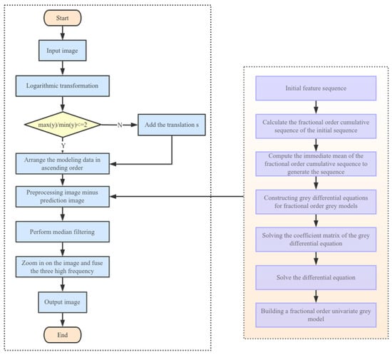
Figure 1.
Algorithm flowchart.
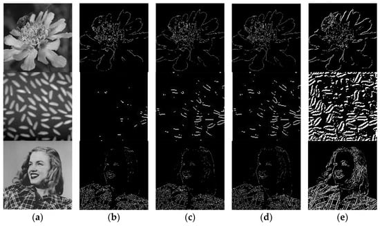
Figure 2.
Edge detection results are created by using several algorithms. Column (a) lists original images of flower, rice, and Marilyn; columns (b–d) are detection results, respectively, by using the classical operators Roberts, Prewitt, and Sobel, and column (e) shows the results obtained by using our algorithm.
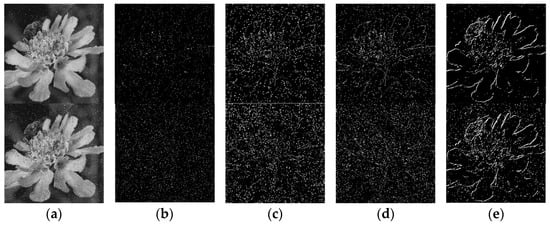
Figure 3.
Edge detection results for the images with salt and pepper noise. The top and bottom images in column (a) are the images added with salt and pepper noise representatively with noise densities of 0.01 and 0.03. Columns (b–d) are the detection results generated by using Roberts, Prewitt, and Sobel, respectively, and column (e) is the detection results generated by using our algorithm.
4.1. Image Edge Detection Effect
We used classical operators for the edge extraction of the images of a flower, rice grains, and Marilyn, and it is not difficult to see from Figure 2 that these operators can extract the general outline of the images, but there are discontinuities and missed detections at the edge details. In the flower edges extracted by the Roberts operator, the petal edge at the bottom right is significantly missing, and the bee outline above the stamen is blurred. Among the flower edges extracted using the Prewitt and Sobel operators, the integrity is better than that of the Roberts operator, and the general outline of the bee can be seen. The edges extracted by using our algorithm have a clearer and more complete outline of the bee than those extracted with the other three operators. The Roberts operator cannot extract most of the rice contours, and the number of rice grains that can be extracted is very limited. The number of rice grains extracted by using the latter Prewitt and Sobel operators is slightly more than those extracted using the Roberts operator, and the edges are clear; the best edge extraction among these three operators is Sobel. Our algorithm can extract more rice grains with clearer edges than the three classical operators. The Roberts operator can extract only part of the edges of Marilyn’s head, with serious details missing, and almost no eyebrows and hair are extracted, while the Prewitt and Sobel operators have similar results and can extract the outer edges of the hair outline, but the edges are not continuous and lose more hair details. By contrast, our algorithm can extract the majority of the edges of Marilyn’s head and clothes, and the edge extraction is more complete, and the hair details are clearly visible.
4.2. Noise Image Edge Detection Effect
We chose the same images as the above experiments for noisy image edge detection. First, the images were processed using the imnoise function in MATLAB to add pretzel noise with noise densities of 0.01 and 0.03, respectively. The results of edge extraction using the classical edge detection methods and our method for the image after adding noise are shown in Figure 3, respectively. Column (b) is detected using the Roberts operator, and as the result shows, one can hardly see the edge of the flower. Column (c) shows the results of this experiment using the Prewitt operator, and as can be seen, the discontinuous edge is detectable, but there is a considerable amount of noise. The results of column (d) using the Sobel operator are the best among the three classical operators, but they also have much noise and are affected by the noise density. In contrast, the edges of the flower detected using our algorithm are complete, accurately located, and less affected by noise. It can be concluded that our method can better extract edge information from noisy images at different pretzel noise densities, while the noise density size has little effect on our method.
5. Conclusions
Image edge detection is the foundation for extracting image characteristics and analyzing and comprehending images, and the quality of image edge detection has a direct impact on the outcome of subsequent image processing. Therefore, it is an important task to find edge detection methods that are accurate in localization, do not miss detection, and are insensitive to noise. In the research of grey prediction systems, fractional-order accumulation is a hot spot of researchers’ attention in recent years. In this paper, we tested and explored the application of a fractional-order cumulative grey model combined with wavelet analysis for image edge detection, and we conducted a series of experiments to evaluate the algorithm’s noise sensitivity and edge detection effect. The results show that the image edge continuity, completeness, and noise resistance using different conventional edge detection operators have their own characteristics. Our algorithm outperforms other classical edge detection operators in terms of detection effect and has the advantages of a novel idea, noise resistance, and rich edge information, which fully proves the wide feasibility and effectiveness of grey system theory in the field of image processing and provides a new idea for image edge detection.
Author Contributions
Conceptualization, M.-Y.P. and L.-N.J.; methodology, M.-Y.P.; writing—original draft preparation, L.-N.J. All authors have read and agreed to the published version of the manuscript.
Funding
This research received no external funding.
Institutional Review Board Statement
Not applicable.
Informed Consent Statement
Not applicable.
Data Availability Statement
The data used to support the findings of this study are available from the corresponding author upon request.
Acknowledgments
The authors thank the editors and anonymous reviewers for their useful comments and suggestions, which helped to improve this paper. At the same time, thank Nanjing Normal University for providing the equipment needed for the experiments. The authors are grateful to W. L. Xie for his assistance and valuable comments on the experiments.
Conflicts of Interest
The authors declare no conflict of interest.
References
- Zhou, R.G.; Liu, D.Q. Quantum Image Edge Extraction Based on Improved Sobel Operator. Int. J. Theor. Phys. 2019, 58, 2969–2985. [Google Scholar] [CrossRef]
- Liu, Y.; Long, Y. Image Edge Extraction Based on Fuzzy Theory and Sobel Operator. In Proceedings of the 2016 IEEE 20th International Conference on Computer Supported Cooperative Work in Design (CSCWD) IEEE, Nanchang, China, 14–16 May 2016; pp. 373–378. [Google Scholar]
- Papari, G.; Petkov, N. Edge and Line Oriented Contour Detection: State of the Art. Image Vis. Comput. 2011, 29, 79–103. [Google Scholar] [CrossRef]
- Roberts; Lawrence, G. Machine Perception of Three-Dimensional Solids; Massachusetts Institute of Technology: Cambridge, MA, USA, 1963. [Google Scholar]
- Sobel, I. Camera Models and Machine Perception; Stanford University: Stanford, CA, USA, 1970. [Google Scholar]
- Prewitt, J.M.S. Object Enhancement and Extraction. In Picture Processing and Psychopictorics; Academic Press: Cambridge, MA, USA, 1970; pp. 75–149. [Google Scholar]
- Parker, J.R. Algorithms for Image Processing and Computer Vision; John Wiley & Sons: Hoboken, NJ, USA, 2010. [Google Scholar]
- Canny, J. A Computational Approach to Edge Detection. IEEE Trans. Pattern Anal. Mach. Intell. 1986, 8, 679–698. [Google Scholar] [CrossRef] [PubMed]
- Liang, L.R.; Looney, C.G. Competitive Fuzzy Edge Detection. Appl. Soft Comput. 2003, 3, 123–137. [Google Scholar] [CrossRef]
- Draghici, S. A Neural Network Based Artificial Vision System for Licence Plate Recognition. Int. J. Neural Syst. 1997, 8, 113–126. [Google Scholar] [CrossRef]
- Feng, L.; Suen, C.Y.; Tang, Y.Y.; Yang, L.H. Edge Extraction of Images by Reconstruction Using Wavelet Decomposition Details at Different Resolution Levels. Int. J. Pattern Recognit. Artif. Intell. 2000, 14, 779–793. [Google Scholar] [CrossRef]
- Pu, Y.F.; Wang, W.X.; Zhou, J.L.; Wang, Y.Y.; Jia, H.D. Fractional Differential Approach to Detecting Textural Features of Digital Image and Its Fractional Differential Filter Implementation. Sci. China Ser. F-Inf. Sci. 2008, 51, 1319–1339. [Google Scholar] [CrossRef]
- Tian, D.; Wu, J.F.; Yang, Y.J. A Fractional-Order Laplacian Operator for Image Edge Detection. Appl. Mech. Mater. 2014, 536, 55–58. [Google Scholar] [CrossRef]
- Lavin-Delgado, J.E.; Solis-Perez, J.E.; Gomez-Aguilar, J.F.; Escobar-Jimenez, R.F. A New Fractional-Order Mask for Image Edge Detection Based on Caputo-Fabrizio Fractional-Order Derivative without Singular Kernel. Circuits Syst. Signal Process. 2020, 39, 1419–1448. [Google Scholar] [CrossRef]
- Hacini, M.; Hacini, A.; Akdag, H.; Hachouf, F. A 2d-Fractional Derivative Mask for Image Feature Edge Detection. In Proceedings of the 2017 International Conference on Advanced Technologies for Signal and Image Processing (ATSIP) IEEE, Fez, Morocco, 22–24 May 2017; pp. 1–6. [Google Scholar]
- Wang, Z.M.; Su, J.Y.; Zhang, P. Image Edge Detection Algorithm Based on Wavelet Fractional Differential Theory. In Proceedings of the 35th Chinese Control Conference, Chengdu, China, 27–29 July 2016; pp. 10407–10411. [Google Scholar]
- Deng, J.-L. Control Problems of Grey Systems. Syst. Control. Lett. 1982, 1, 288–294. [Google Scholar]
- Liu, Y.; Pan, F.; Xue, D.; Nie, J. A Novel Fractional-Order Discrete Grey Model with Initial Condition Optimization and Its Application. In Proceedings of the 2021 33rd Chinese Control and Decision Conference (CCDC) IEEE, Kunming, China, 22–24 May 2021; pp. 2007–2012. [Google Scholar]
- Meixin, H.; Caixia, L. A Variable-Order Fractional Discrete Grey Model and Its Application. J. Intell. Fuzzy Syst. 2021, 41, 3509–3522. [Google Scholar] [CrossRef]
- Miao, M.; Yanyu, F.; Songyun, X.; Chongyang, H.; Xinwu, L. A Novel Algorithm of Image Edge Detection Based on Grey System Theory. J. Image Graph. 2003, 8, 1136–1139. [Google Scholar]
- He, R.; Huang, D.; Chen, J. Image Edge Detection Based on Grey Prediction Model. J. Northwestern Polytech. Univ. 2005, 23, 15–18. [Google Scholar]
- Li, J.-F.; Dai, W.-Z. Research of Image Edge Detection and Application Based on Grey Prediction Model. In Proceedings of the 2007 International Conference on Wavelet Analysis and Pattern Recognition IEEE, Beijing, China, 2–4 November 2007; Volume 1, pp. 286–291. [Google Scholar]
- Xie, S.Y.; Zhang, K.; Zhang, N. A New Method of Image Denoising Based on Grey Prediction. Microelectron. Comput. 2006, 12, 151–153. [Google Scholar]
- Wu, C.-C.; Peng, G.-H. Image Edge Extraction Algorithm Based on Ugm Grey Prediction Model. Comput. Eng. Appl. 2012, 48, 214–217. [Google Scholar]
- Wang, Q.; Wang, T.; Zhang, K. Image Edge Detection Based on the Grey Prediction Model and Discrete Wavelet Transform. Kybernetes 2012, 41, 643–654. [Google Scholar] [CrossRef]
- Kang, Y.; Mao, S.; Zhang, Y. Variable Order Fractional Grey Model and Its Application. Appl. Math. Model. 2021, 97, 619–635. [Google Scholar]
- Gao, M.; Mao, S.; Yan, X.; Wen, J. Estimation of Chinese CO2 Emission Based on a Discrete Fractional Accumulation Grey Model. J. Grey Syst. 2015, 27, 114–130. [Google Scholar]
- Mao, S.; Gao, M.; Xiao, X.; Zhu, M. A Novel Fractional Grey System Model and Its Application. Appl. Math. Model. 2016, 40, 5063–5076. [Google Scholar] [CrossRef]
- Yang, Y.; Xue, D. Continuous Fractional-Order Grey Model and Electricity Prediction Research Based on the Observation Error Feedback. Energy 2016, 115, 722–733. [Google Scholar] [CrossRef]
- Xie, W.; Liu, C.; Wu, W.-Z.; Li, W.; Liu, C. Continuous Grey Model with Conformable Fractional Derivative. Chaos Solitons Fractals 2020, 139, 110285. [Google Scholar] [CrossRef]
- Xie, W.; Wu, W.Z.; Liu, C.; Goh, M. Generalized Fractional Grey System Models: The Memory Effects Perspective. ISA Trans. 2022, 126, 36–46. [Google Scholar] [CrossRef] [PubMed]
- Wu, L.; Liu, S.; Yao, L.; Yan, S.; Liu, D. Grey System Model with the Fractional Order Accumulation. Commun. Nonlinear Sci. Numer. Simul. 2013, 18, 1775–1785. [Google Scholar] [CrossRef]
- Wu, L.F.; Liu, S.F.; Yao, L.G. A Discrete Grey Model Based on Fractional Order Cumulants. Syst. Eng. Theory Pract. 2014, 34, 1822–1827. [Google Scholar]
- Kumar, K.; Mustafa, N.; Li, J.-P.; Shaikh, R.A.; Khan, S.A.; Khan, A. Image Edge Detection Scheme Using Wavelet Transform. In Proceedings of the 2014 11th International Computer Conference on Wavelet Actiev Media Technology and Information Processing (ICCWAMTIP) IEEE, Chengdu, China, 19–21 December 2014; pp. 261–265. [Google Scholar]


Publisher’s Note: MDPI stays neutral with regard to jurisdictional claims in published maps and institutional affiliations. |
© 2022 by the authors. Licensee MDPI, Basel, Switzerland. This article is an open access article distributed under the terms and conditions of the Creative Commons Attribution (CC BY) license (https://creativecommons.org/licenses/by/4.0/).