Environmental Sound Classification Algorithm Based on Region Joint Signal Analysis Feature and Boosting Ensemble Learning

Abstract

Environmental sound classification is an important branch of acoustic signal processing. In this work, a set of sound classification features based on audio signal perception and statistical analysis are proposed to describe the signal from multiple aspects of the time and frequency domain. Energy features, spectral entropy features, zero crossing rate (ZCR), and mel-frequency cepstral coefficient (MFCC) are combined to form joint signal analysis (JSA) features to improve the signal expression of the features. Then, based on the JSA, a novel region joint signal analysis feature (RJSA) for environment sound classification is also proposed. It can reduce feature extraction computation and improve feature stability, robustness, and classification accuracy. Finally, a sound classification framework based on the boosting ensemble learning method is provided to improve the classification accuracy and model generalization. The experimental results show that compared with the highest classification accuracy of the baseline algorithm, the environmental sound classification algorithm based on our proposed RJSA features and ensemble learning methods improves the classification accuracy, and the accuracy of the LightGBM-based sound classification algorithm improves by 14.6%.

1. Introduction

Sound is one of the most important carriers of information. An audio signal in a real environment contains a lot of environment-related information. Based on experience and ability, humans can efficiently recognize the surrounding environment from sounds. The recognition and classification of an audio signal, i.e., the identification and determination of the recorded sound’s environmental label, can be used in a range of security monitoring systems such as audio surveillance, anomaly detection, and risk prevention and control. With the development of information technology, particularly the advancement of pattern recognition theory and methods, artificial intelligence systems have become widely used in a variety of scientific and technical fields. Automatic recognition of environmental sound is a key direction for environmental sound research for signal and information processing [1].

Generally, environmental sound classification algorithms are composed of both feature extraction and classification model (two parts). Audio features used for sound classification must be able to capture the essential characteristics of various types of audio signals efficiently. These features must be robust and have complete signal characterization capabilities for complex audio signals. Feature extraction is an important part of sound classification algorithms. The mainstream feature extraction methods are basically based on signal processing and transformation, including waveform structure feature extraction in the time domain, spectral analysis, and higher-order statistics analysis in the frequency domain, short-time Fourier transform and wavelet analysis in the time-frequency domain, and nonlinear feature extraction of signals. For decades, the potential of the methods mentioned above has been fully explored with promising results. Generalized auditory features include zero crossing rate (ZCR), short-term energy (STE), linear prediction coefficient (LPC), spectral centroid (SC), mel-frequency cepstral coefficients (MFCC), spectral flux (SF), spectral irregularity (SI), spectral entropy (SE), and spectral contrast (SC). A well-performing classifier is required for an excellent recognition system in addition to a feature set with clustering and scattering. The classifier makes some kind of transformation and mapping of the feature vectors from the feature space to the target type space. By using a set number of environmental sound signals as training samples, the classifier training module determines the values of the parameters in the classifier [2,3,4,5,6,7,8]. The primary classifiers utilized in the algorithms include k-nearest neighbor (KNN)-based classifiers [9,10,11,12,13], multilayer perceptron (MLP)-based classifiers [14,15], convolutional recurrent neural network (CRNN)-based classifiers [16,17,18,19,20], convolutional neural network (CNN)-based classifiers [21,22,23,24,25,26,27], support vector machine (SVM)-based classifiers [28,29,30,31,32,33], and Gaussian mixed model (GMM)-based classifiers [34,35,36]. The information that a model can provide generally comes from two aspects, the information contained in the training data and the prior information that people supply.

Audio classification research dates back to the 1990s when algorithms based on the self-organizing neural network and nearest neighbor criterion were first applied to automatic sound retrieval and audio classification systems [37]. In 1997, the concept of sound classification was first introduced and established by Sawhney and Maes, researchers at the Multimedia Laboratory at MIT [38]. The development of sound classification algorithms mainly focuses on two aspects of feature extraction and classification models, and machine learning-based sound classification algorithms have received considerable attention. Chachada and Kuo investigated and summarized sound classification algorithms based on machine learning. Eleven combinations of feature extractors and classifiers were tested on a sound dataset with 37 sound types. The experimental results reveal that a combination of MFCC and SVM classifiers produces the best classification results, with a classification accuracy of 76.74%. The algorithm based on the spectrogram and feedforward neural network classifier was the poorest, and the classification accuracy did not reach 40%. It was pointed out that ensemble multiple classifiers to learn complementary feature combinations for sound classification is a future research direction [39]. J. Piczak implemented the classification of the ESC-10 dataset based on KNN, SVM, and RF classification methods using MFCC and ZCR features. The accuracy of the classification algorithm based on RF achieves the best classification result. Through a five-fold cross validation, the accuracy of the algorithm based on KNN was 66.7%, the accuracy of the algorithm based on SVM was 67.5%, the accuracy of the algorithm based on the RF was 72.7%. Shaukat et al. [40] used ensemble-learning algorithms to achieve excellent performance in the classification of daily sound events. In recent years, ensemble-learning algorithms based on boosting method have advanced and progressed. Some excellent boosting ensemble-learning algorithms have demonstrated great performance in classification and regression task.

Based on the joint analysis of audio signal time-frequency domain perception and statistics, an environmental sound classification algorithm with novel region joint signal analysis (RJSA) features and boosting ensemble learning is proposed in this paper. The main contributions of our research are as follows:

• A signal analysis (SA) feature based on joint analysis of audio signal perception and statistics is proposed. This feature consists of the continuous frame correlation feature, the signal positive and negative waveform amplitude similarity feature, the average amplitude feature of energy fluctuations in the time domain, and the adjacent frame correlation feature, the sub-band energy fluctuation amplitude feature in the frequency domain. Combining existing signal statistical analysis features, the joint signal analysis (JSA) feature is formed to improve the signal description capability of features and the classification accuracy.
• A novel region joint signal analysis feature (RJSA) for environment sound classification is proposed. Determine the audio signal energy threshold first and the signals for the region where the energy is lower than the threshold are dropped to reduce the influence of redundant signals on the target audio signal. Performing feature extraction for the region where the signal energy is greater than the threshold to reduce feature extraction computation, improve feature stability, robustness, and classification accuracy.
• A sound classification framework based on the RJSA feature and boosting ensemble learning method is provided. The popular boosting ensemble-learning algorithms are adopted to classify environmental sound; and the model robustness, algorithm generalization ability, stability, and classification accuracy are improved.

The rest of the paper is organized as follows. The JSA feature is introduced in Section 2. Section 3 focuses on the RJSA feature based on signal energy. Section 4 presents the framework for environment sound classification based on boosting the ensemble-learning algorithm and RJSA feature. Section 5 presents the experimental results and Section 6 gives the conclusions and directions for future research in our work.

2. Joint Signal Analysis (JSA) Feature

Audio features include time domain and frequency domain features. Time domain features are typically processed on the signal’s sampled values and do not require any change of the original audio signal. This is one of the most basic and traditional ways for extracting audio features. Typical time domain features include ZCR-based features, amplitude-based features, energy-based features, etc. The frequency domain features are generally closely related to timbre, which is based on the Fourier transform. It can be further divided into spectral envelope and spectral structure correlation features, statistical features, and coefficient features.

In the process of audio signal analysis, the time domain waveform map and spectrogram of the audio signal have definite distinctions after visualization of the sound signal, in addition to the sound that can be directly distinguished by auditory perception. The spectrograms of different types of sound signal examples in the ESC-10 dataset are given in Figure 1. The horizontal axis of the spectrogram is time, the vertical axis of the spectrogram is frequency, and the amplitude is indicated by color.

The spectrogram can reflect at the same time the change of frequency and amplitude of the signal with time. A set of sound classification features based on perception and statistical analysis are proposed by visualizing and analyzing the time domain waveform and spectrograms of the audio signal. The proposed new feature is the signal analysis (SA) feature. This feature consists of the continuous frame correlation feature, the signal positive and negative waveform amplitude similarity feature, the average amplitude feature of energy fluctuations in the time domain, and the adjacent frame correlation feature, the sub-band energy fluctuation amplitude feature in the frequency domain. The features are extracted from the time domain and frequency spectrum, adjacent frames, and sub-bands. Then, existing features including sub-band energy distribution ratio, spectral entropy, cross entropy, and the short-time energy in the time domain, ZCR, and MFCC are combined to form a JSA feature.

2.1. Signal Analysis (SA) Feature

The proposed features in SA will be described in detail in this section.

2.1.1. Time Domain Feature

Signal time domain features generally do not require a formal transformation of the original audio signal, processed on the sampled values of the signal itself. Based on the time domain waveform analysis of audio signals, the continuous frame correlation feature, the signal positive and negative waveform amplitude similarity feature, and the time domain signal energy fluctuation rate feature are proposed. Assume that x represents the signal time domain amplitude, N represents the frame length of each signal frame, k denotes the index value of the number of frames, and K is the total number of frames.

The continuous frame correlation feature is expressed as:

$$f_{T\_corr}=\frac{1}{K}{\displaystyle \sum _{k=1}^K\left(\frac{{\displaystyle \sum _{n=1}^{N}x(n,k)\cdot x(n,k+1)}}{\sqrt{{\displaystyle \sum _{n=1}^N{x}^2(n,k)\cdot }{\displaystyle \sum _{n=1}^N{x}^2(n,k+1)}}}\right)}$$

(1)

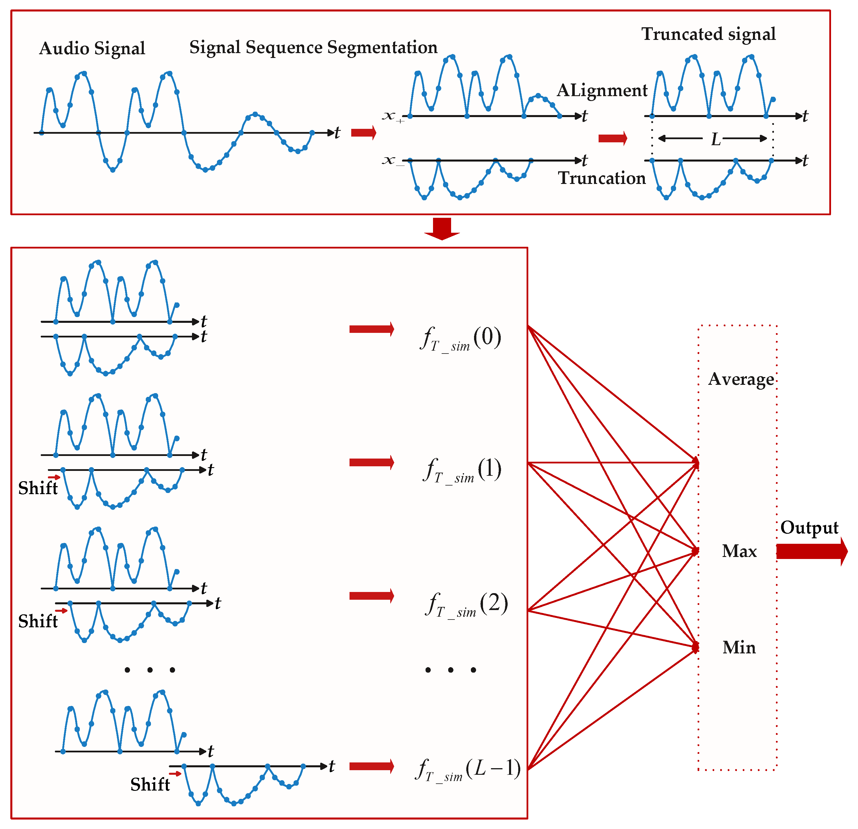
The signal positive and negative waveform amplitude similarity feature computes the symmetry of the signal waveform about the positive and negative signals of the time axis, which is directly expressed as the similarity of the normalized audio signal with positive amplitude to the negative amplitude. The signal positive and negative waveform amplitude similarity feature is calculated as follows:

$$f_{T\_sim}(l)=-\frac{{\displaystyle \sum _{i=1}^{L-l}{x}_{+}(i)\cdot x_{-}(i)}}{\sqrt{{\displaystyle \sum _{i=1}^{L-l}{x}_{+}^2(i)\cdot {\displaystyle \sum _{i=1}^{L-l}{x}_{-}^2(i)}}}}0\le l\le L-1$$

(2)

$x_{+}$ and $x_{-}$ denotes the positive and negative signals that correspond to the mutually overlapping parts of the sequence after shifting, as shown in Figure 2. In Figure 2, i is the index of the signal sampling point and L is the signal length. The signal positive and negative waveform amplitude similarity feature includes the mean value, maximum value, and minimum values of waveform amplitude similarity.

The similarity of waveform amplitudes of the audio signal is expressed as:

$$f_{T\_ave}=\frac{1}{L}{\displaystyle \sum _{l=1}^L{f}_{T\_sim}(l)}$$

(3)

$$f_{T\_\max }=\max (f_{T\_sim}(0),f_{T\_sim}(1)\cdots f_{T\_sim}(L-1))$$

(4)

$$f_{T\_\min }=\min (f_{T\_sim}(0),f_{T\_sim}(1)\cdots f_{T\_sim}(L-1))$$

(5)

$$f_{T\_PNC}=[f_{T\_ave},f_{T\_\max },f_{T\_\min }]$$

(6)

The average amplitude feature of time domain energy fluctuations mainly reflects the speed of the process of signal energy rise and decline, and the average amplitude of time domain energy decline is expressed as:

$$f_{T\_des}=\frac{{\displaystyle \sum _{E(k)>E(k+1)}\left({\displaystyle \sum _{n=1}^N|x(n,k+1)|-{\displaystyle \sum _{n=1}^N|x(n,k)|}}\right)}}{{\displaystyle \sum _{E(k)>E(k+1)}\mathrm{sgn}(E(k)-E(k+1))}}$$

(7)

$$E(k)={\displaystyle \sum _{n=1}^N|x(n,k)|}$$

(8)

where ${\displaystyle \sum _{E(k)>E(k+1)}\mathrm{sgn}(E(k)-E(k+1))}$ denotes the number of times the energy of the signal frame decreases. $\mathrm{sgn}[\cdot ]$ is the sign function, namely:

$$\mathrm{sgn}[x]=\{\begin{array}{ll}1& x\ge 0\\ -1& x<0\end{array}$$

(9)

The average amplitude of time domain energy rise is expressed as:

$$f_{T\_ins}=\frac{{\displaystyle \sum _{E(k)<E(k+1)}\left({\displaystyle \sum _{n=1}^N|x(n,k+1)|-{\displaystyle \sum _{n=1}^N|x(n,k)|}}\right)}}{{\displaystyle \sum _{E(k)<E(k+1)}\mathrm{sgn}(E(k+1)-E(k))}}$$

(10)

where ${\displaystyle \sum _{E(k)<E(k+1)}\mathrm{sgn}(E(k+1)-E(k))}$ denotes the number of times the energy of the signal frame increase.

2.1.2. Frequency Domain Feature

The time domain analysis method has the advantages of simplicity and clear physical meaning. However, since some of the more important perceptual features of sound signals are reflected in the power spectrum, frequency domain analysis is also very important compared to time domain analysis.

The spectral structure of environmental sound can reflect the differences in the acoustic properties of environmental sound. The research in [1] provides spectrum analysis of sound samples in five different types of sound environments, and the results demonstrate that the spectral energy of environmental sound in vehicles (cabs and buses) is more concentrated below 1 kHz, where low frequency energy below 200 Hz is more significant. Environmental sound in public places (restaurants, shopping malls, supermarkets, etc.) has a wide frequency band, with the majority of spectral energy concentrated below 3000 Hz. Environmental sound energy in quiet indoor areas (study rooms, laboratories) is small, mainly distributed at a low frequency of about 100 Hz. The distribution band of outdoor traffic environment sound (lanes, intersections) is wide, with more energy distributed below 2000 Hz and a slightly prominent spectrum near 3 kHz and 5 kHz, owing to the presence of mechanical sounds of vehicles running on the road, tire noise, and horn sound, etc. The energy of pure speech is more concentrated in the low and middle frequency band of 1.5 kHz and is more evenly distributed. The spectral distribution of typical environmental sound is different, and the spectral structure reflects the differences in the acoustic properties of the environmental sound [2].

Since the energy distribution of different signals is concentrated in different frequency regions, the sub-band adjacent frame correlation feature and the energy fluctuation amplitude feature are proposed based on frequency domain signals. The correlation and fluctuation of the audio signal are described from each frequency band in the signal frequency domain. In the calculation process of the sub-band adjacent frame correlation feature and energy fluctuation rate feature, the audio signal is divided into frames first, processed by window function, and then the Fourier transform of the signal is performed, and the transformed signal is uniformly divided in the frequency band. After the division of the signal, the adjacent frame correlation feature is expressed as follows:

$$f_{S\_corr}(j)=\frac{{\displaystyle \sum _{m=1}^M{X}_j(m,k)\cdot X_j(m,k+1)}}{\sqrt{{\displaystyle \sum _{m=1}^M{X}_j^2(m,k)\cdot }{\displaystyle \sum _{m=1}^M{X}_j^2(m,k+1)}}}$$

(11)

where X represents the fast Fourier transform of x, m denotes the frequency point index within each band, and j denotes the frequency band index.

The sub-band energy fluctuation amplitude feature is calculated as follows:

$$f_{S\_des}(j)=\frac{{\displaystyle \sum _{E(k)>E(k+1)}\left({\displaystyle \sum _{m=1}^M|X_j(m,k+1){|}^2-{\displaystyle \sum _{m=1}^M|X_j(m,k){|}^2}}\right)}}{{\displaystyle \sum _{E(k)>E(k+1)}\mathrm{sgn}(E(k)-E(k+1))}}$$

(12)

$$E(k)={{\displaystyle \sum _{m=1}^M|X_j(m,k){|}^2}}^{}$$

where ${\displaystyle \sum _{E(k)>E(k+1)}\mathrm{sgn}(E(k)-E(k+1))}$ denotes the number of times the energy of the signal frame declines. The rising rate of the time domain energy is expressed as:

$$f_{S\_ins}=\frac{{\displaystyle \sum _{E(k)<E(k+1)}\left({\displaystyle \sum _{m=1}^M|X_j(m,k+1){|}^2-{\displaystyle \sum _{m=1}^M|X_j(m,k){|}^2}}\right)}}{{\displaystyle \sum _{E(k)<E(k+1)}\mathrm{sgn}(E(k+1)-E(k))}}$$

(13)

where ${\displaystyle \sum _{E(k)<E(k+1)}\mathrm{sgn}(E(k+1)-E(k))}$ indicates the number of times the energy of the signal frame rises.

Based on the analysis of the time domain waveform and spectrogram of environmental sound signal, the continuous frame correlation feature, the signal positive and negative waveform amplitude similarity feature, and the time domain signal energy fluctuation rate feature are proposed to describe the correlation degree of adjacent frame signals, the signal positive and negative amplitude similarity degree in the time domain, and the signal energy fluctuation during the signal change over time. The sub-band adjacent frame correlation feature and the energy fluctuation amplitude feature are proposed to describe the correlation and energy fluctuation levels between adjacent frames in the frequency domain of the band signal. The audio signal is represented in the time domain, frequency domain, single frequency band, adjacent frame relationships, energy variations, and statistical properties.

2.2. Joint Feature

In addition to the SA feature, existing features are adopted to complete signal analysis and description. The signal sub-band entropy and cross entropy features can effectively represent the random characteristics of a single band as well as the correlation characteristics between adjacent bands, while the sub-band energy and energy distribution ratio features can reflect the energy distribution. Therefore, these four sub-band features are used to characterize the band energy distribution, the random properties, and the correlation properties between adjacent bands of the signal. The perceptual and statistical analysis features, the sub-band energy distribution ratio, spectral entropy, cross entropy, and the short-time energy in the time domain, ZCR, and MFCC are combined to form a JSA feature.

A comprehensive description of the audio signal is given in terms of time domain signal energy, similarity between adjacent frames, positive and negative amplitude symmetry, amplitude fluctuation rate, number of transitions of zero, frequency domain band energy distribution, signal stochastic properties, correlation between adjacent bands, adjacent frame correlation, spectral sub-band fluctuation rate, and cepstrum domain characteristics. The JSA feature is expressed as:

$$\begin{array}{cc}\hfill f_{Co-A}=& [f_{S\_sed},f_{T\_E},f_{S\_BE},f_{S\_BCE},f_{S\_corr},f_{S\_E},f_{S\_des},\hfill \\ & f_{S\_ins},f_{T\_corr},f_{T\_PNC},f_{T\_des},f_{T\_ins},f_{T\_zcr},f_{MFCC}]\hfill \end{array}$$

(14)

3. Region Joint Signal Analysis (RJSA) Feature

In the process of environmental sound recognition, there are some interfering signals or redundant signals, which can affect the accuracy of sound recognition. In the perception of environmental sound, the surrounding environment can often be identified by some of the significantly representative sound signals, for example, the surrounding environment can be generally identified as a traffic environment by the sound of car sirens and motor vehicle driving noise.

To reduce the influence of the interfering signals and redundant signal, the RJSA feature is proposed to improve the stability and effectiveness of the JSA feature. RJSA is based on the Pareto principle. Pareto proposed the famous Pareto principle in 1906, also known as the 80/20 rule [41,42]. Since its introduction, the Pareto principle has been widely applied in different fields and has been proven to be correct in the majority of cases after numerous experimental tests. In any case, the main outcome of things depends on only a small number of factors. In any factor that produces some common effect, a relatively small number of factors contribute most of the effect. The majority of measurable improvements are the product of a limited number of quality improvement projects, those critical few factors. The majority of programs belong to the useful majorities, which are typically several orders of magnitude less effective than the critical few factors.

The Pareto principle provides a relatively clear proportional relationship, but since it is based on a large amount of statistical data, it may not always reflect a strict 80/20 proportional relationship. This proportional relationship might be biased for two reasons. First of all, it is possible to find the 80/20 rule based on the classification of the data. If the classification of the data is not precise and complete, the analysis’s results may be biased. In addition, if the number of sub-samples obtained is insufficient, the analytical results may be biased. However, as long as the corresponding statistics are sufficient and the data classification analysis is generally reasonable, it can be discovered that there is a tendency for a small number of causes to lead to a large number of failures, or for a small number of efforts to achieve the majority of the results. When applying Pareto principle, it is not possible to demand that the data completely satisfy the numbers of 80% and 20%; any situation where a few factors determine the main outcome is consistent with Pareto principle. The main idea of the RJSA feature is using some of the sound signal to replace the complete signal.

Background audio signal is always present in the real world, but not all background sounds contain valid identification information for environmental sounds. As shown in Figure 1, the sound of baby crying, clock ticking, and dog barking with distinct signal characteristics mainly concentrate on the high energy signal segment. Based on the Pareto principle, the RJSA feature is proposed to extract features only for the signals in the energy prominence regions. Using some of the signal features for sound classification, combined with RSA features, the RJSA feature extraction process is shown in Figure 3.

The input signal is first framed and processed with windows, after which the validity of the framed signal is evaluated, and the amplitude of the signal frame with a sum of zero is filtered out to avoid interfering with the calculation of subsequent features. The energy of each signal frame is calculated and the average energy of the signal frame is derived. Based on the defined gain factor and the average energy of the signal, the energy threshold of the signal corresponding to the energy prominence region is calculated. The energy of the signal frames is compared with the energy threshold. The signal frames with energy greater than the threshold value are remained, and the signal frames with energy less than the threshold value are dropped, then the JSA feature is extracted from energy prominence regions. The extracted features are RJSA features, which can be used for environmental sound classification.

The frame average energy calculation during the energy prominence regions computation is expressed as:

$$AE=\frac{1}{K}{\displaystyle \sum _{k=1}^K\left({\displaystyle \sum _{n=1}^N{x}^2(n)}\right)}$$

(15)

The energy threshold is expressed as:

$$ET=\alpha \cdot AE$$

(16)

The value of the energy threshold can be changed by adjusting the gain factor α. For a fixed frame signal, the range of energy prominence regions is reduced by a higher energy threshold, and the energy of the signal used for feature extraction is more prominent. By comparing frame energy to the energy threshold, the signal frames with higher energy and the signal frames with lower energy are classified into two groups. The high-energy frame signals constitute the energy prominence regions.

$$ESR=\left\{x_k|E_{x_k}>ET\right\}$$

(17)

The RJSA feature is obtained through feature extraction from the energy prominence regions.

4. Ensemble-Learning Algorithm Based on Boosting Method

Tree-based classifiers were first applied to the background noise classification task in 2014, and the algorithms showed great advantages in terms of running time and classification accuracy. Although neural networks have revived and become popular in recent years, boosting-based ensemble-learning algorithms still have a distinct advantage in circumstances where the training sample size is restricted, the needed training time is short, and the knowledge of tuning parameters is weak. Boosting-based algorithms have been developed in recent years, but they have received less attention in sound signal processing. Therefore, we introduce boosting algorithms into sound classification to explore the effectiveness of the algorithms.

Boosting is a method of boosting weak learners into strong learners. In the classification problem, it learns multiple classifiers by changing the weights of the training samples and combining these classifiers into linear combinations to improve the performance of classification. The schematic diagram of the gradient boosting algorithm is shown in Figure 4. Boosting methods train the base model after transforming the training set each time, and then combine all of the base model prediction results.

Chen proposed the eXtreme Gradient Boosting (XGBoost) method [43,44] in March 2014. In January 2017, Microsoft published the first stable version of the Light Gradient Boosting Machine (LightGBM) [45], and in April 2017, Yandex open-sourced the Categorical Features Gradient Boosting (CatBoost) method [46,47]. In fact, XGBoost, LightGBM, and CatBoost are different implementations of the gradient boosting decision tree (GBDT) method, with different optimizations for the same purpose. XGBoost, LightGBM, and CatBoost the current state of the art (SOTA) boosting algorithms, all of which can be classified into the class of gradient-boosting decision-tree algorithms.

4.1. Gradient Boosting Decision Tree Method

The GBDT algorithm combines a decision tree with gradient boosting [48,49], The value of the negative gradient of the loss function is used in the current model as the residual approximation in the algorithm. The idea of the algorithm is to keep fitting the residuals so that the residuals continually decrease. The negative gradient value of the loss function for the i-th sample of the m-th iteration is:

$$r_{m,i}=-\eta {\left[\frac{\partial L(y_i,f(x_i))}{\partial f(x_i)}\right]}_{f(x_i)=f_{m-1(x_i)}}$$

(18)

Fit the regression tree to $r_{m,i}$ to obtain the m-th tree, whose corresponding leaf node region is $R_{j,m}$. Calculate the optimal output value ${\gamma }_{j,m}$ for each leaf node region sample.

$${\gamma }_{jm}=\arg \underset{\gamma }{\min }{\displaystyle \sum _{x_i\in R_{jm}}^{}L(y_i,f_{m-1}(x_i)+\gamma )}$$

(19)

Then, the tree fitting function for this iteration is:

$$h_m(x)=\eta {\displaystyle \sum _{j=1}^J{\gamma }_{jm}I(x\in R_{jm})}$$

(20)

Thus, obtaining the final strong learner:

$$F(x)=f_M(x)=f_0(x)+\eta {\displaystyle \sum _{m=1}^M{\displaystyle \sum _{j=1}^J{\gamma }_{jm}I(x\in R_{jm})}}$$

(21)

4.2. XGBoost, LightGBM and CatBoost

XGBoost is an improvement of the original version of the GBDT algorithm, while LightGBM and CatBoost are further optimizations based on the XGBoost, which have their own advantages in terms of accuracy and speed. All three methods are ensemble learning frameworks supported by decision trees. The main characteristics and important parameters of the three methods are shown in

Table 1. The main characteristics and important parameters of XGBoost, LightGBM, and CatBoost.

		XGBoost	LightGBM	CatBoost
Common Characteristics		1. Gradient-boosting decision-tree algorithm 2. based on decision trees 3. greedy thoughts
Improvements & Benefits		1. parallel computing 2. second-order derivative of the loss function 3. linear model support; 4. regular term adding 5. shrinkage factor 6. column sampling 7. handling missing values	1. histogram algorithm 2. gradient-based one-side sampling (GOSS) 3. exclusive feature bundling (EFB) 4. leaf-wise algorithm 5. data parallel acceleration 6. cache optimizing	1. reducing hyper parameters tuning 2. interface for integration with scikit, as well as R and command-line interface 3. supporting categorical variables 4. self-defining loss functions 5. scalable GPU version 6. efficient deployment
Drawbacks		1. still need to traverse the dataset during the node splitting process 2. high space complexity of the pre-sorting process	1. may grow deeper decision trees in leaf-wise and produce over-fitting 2. sensitivity to noise	1. the processing of categorical features requires a lot of memory and time 2. random number settings influence the model prediction results
Hyper parameter	OC	learning_rate, max_depth, min_child_weight	learning_rate, max_depth, min_data_in_leaf	learning_rate, depth, l2_reg_leaf
	CV	/	categorical_feature	cat_features, one_hot_max_size
	SC	colsample_bytree, subsample, n_estimators	feature_fraction, bagging_fraction, num_iterations	rsm, iterations

Where OC represents the hyperarameter used for overfitting, CV represents the hyperparameter used for categorical values, and SC represents the hyperparameter used for speed control.

. The table lists the common characteristics of the three boosting methods, as well as their respective advantages, drawbacks, and important model parameters.

All three boosting ensemble learning methods can control overfitting by adjusting the learning rate and tree depth. XGBoost is a high-speed computational algorithm with good model performance that can be used in classification and regression problems. LightGBM is faster and more efficient in training, uses less memory, has higher accuracy, and supports parallelized learning and processing of large-scale data. CatBoost uses a strategy that reduces overfitting while ensuring that all datasets are available for learning. It provides excellent performance, better robustness and generality, ease of use, and increased practicality. There is no definitive conclusion on which of these three algorithms is the best [50]. Therefore, we use three boosting ensemble learning methods for classification separately and analyze the applicability of the model by the classification results.

4.3. Algorithmic Framework for Sound Classification Based on Boosting Method

The framework of the RJSA feature and boosting ensemble learning (RJSABE) algorithm is described in detail in this paragraph. The feature extraction and classification process are shown in Figure 5.

In the training process, the signal is firstly framed and windowed, then the energy prominence signal region is extracted by the signal energy threshold. Features are extracted from the time domain, frequency domain and cepstrum domain of the energy prominence signal to obtain the RJSA features, which are composed into a dataset, and the boosting ensemble learning model is trained using the feature dataset. In the prediction process, the corresponding RJSA features are first extracted from the input audio signal, and then the features are fed into the trained model to obtain the output classification results.

5. Experimental Results

In this section, we present the experimental results of the environmental sound classification algorithm based on the RJSA features and boosting ensemble learning methods. First, the environmental sound classification dataset ESC-10 used for the experiments is introduced. The experimental setup for background noise classification algorithm is sequentially presented. After that, we give a comparison of the experimental results of the RJSA feature-based sound classification and the baseline algorithm. In addition, the effect of energy prominence region features on sound classification accuracy was analyzed. Finally, experimental results of the sound classification algorithm framework based on the boosting ensemble learning are given.

5.1. ESC-10 Dataset

The ESC-10 dataset is a labeled environmental sound dataset that can be used to test environmental sound classification algorithms. This dataset contains 10 classes of sound signals. Each class has 40 samples. A total of 400 samples are included. The signal sampling rate is 44.1 kHz. The length of each sample is 5 s, and the total length is about 33 min. There are three common classes of sound, namely: transient sound signals such as clock ticking, dog barking, and sneezing; sound signals with strong harmonic components such as a crowing rooster and crying baby; structured noise such as chainsaw, helicopter, fire crackling, sea waves, and rain. The dataset is arranged into 5 uniformly sized cross validation folds to ensure that signal clips from the same source file are always contained in a single fold. ZCR and MFCC features were used for baseline sound classification algorithms, and experiments were conducted based on three types of classifiers, KNN, SVM, and RF. The five-fold cross validation method was used for the experiments.

5.2. Experimental Setup

The audio signal is divided into frames according to a frame length of 25 ms, with a frame overlap of 50% of the frame length, and pre-processed with the hamming window. The gain factors (α) are taken as (0.2, 0.4, 0.6, 0.8, 1.0, 1.2) by calculating the energy thresholds of the energy prominence regions from the time domain signals. The sampling frequency of the signal is not changed during the signal processing process, and the signal spectrum is divided into 40 sub-band signals in the frequency domain, each with a bandwidth of 551 Hz. The 1-dimensional continuous frame correlation feature, 3-dimensional positive and negative waveform amplitude similarity feature, and 2-dimensional energy fluctuation average amplitude feature are extracted from the signal time domain. The 40-dimensional sub-band spectral continuous frame correlation feature and 80-dimensional sub-band spectral energy fluctuation average amplitude features are extracted from the 40 sub-bands of the signal frequency domain. In addition, the 1-dimensional short time energy feature and1-dimensional ZCR feature are extracted from the time domain, 40-dimensional sub-band energy distribution feature, 40-dimensional sub-band energy, 40-dimensional sub-band spectral entropy feature, 39-dimensional sub-band cross entropy feature are extracted from the signal frequency domain, and 7-dimensional MFCC feature is extracted from the cepstrum domain. A 294-dimensional joint SA feature is formed by all of the features. The RF model is first adopted to validate the effectiveness of the features. The RF model employs 200 sub-estimators.

In the framework of the RJSA feature and boosting ensemble learning (RJSABE) algorithm, the XGBoost model is set to have 200 sub-estimators, the LightGBM model is set to have 200 sub-estimators, and the CatBoost model is set to have 1000 iterations after repeated experiments. Random state is set to 28 for all the classifiers. The metric_period in catboost is set to 100. This parameter controls the frequency of iterations to calculate the values of objectives and metrics. All other parameters are default values to show the advantages of the algorithm in hyperparameter optimization.

The experimental process is implemented by MATLAB on a ThinkServer TS80X for feature extraction and dataset construction, and by PYTHON on an Intel core i7 8th gen laptop for model training and testing process. Machine learning library scikit-learn, xgboost, lightgbm, and catboost are used. The feature dataset contains a total of 400 × 293-dimensional features and the corresponding labels. Experiments were performed using the five-fold cross validation given by the dataset, and the final classification accuracy was obtained by averaging these five classification accuracies.

5.3. Experimental Results

The sounds were classified using the JSA features and RF model first, and the classification results are shown in

Table 2. Sound classification result based on the SA features and RF model.

Baseline-KNN	Baseline-SVM	Baseline-RF	JSA-RF
66.7%	67.5%	72.7%	81.5%

. The left three columns in the table show the baseline classification results, the highest of which is the RF-based sound classification algorithm. The last column shows the sound-classification algorithm based on JSA features and RF model. The environmental sound classification algorithm based on JSA features and RF model improves the classification accuracy by about 9% over the highest baseline. Based on ZCR and MFCC, the signal energy, similarity between adjacent frames, positive and negative amplitude symmetry, amplitude fluctuation amplitude in time domain and sub-band energy distribution, signal stochasticity, adjacent sub-band correlation, adjacent frame correlation, and spectral fluctuation amplitude in the frequency domain are jointed for a comprehensive description of the environmental sound signal. Therefore, the JSA features can effectively improve the classification accuracy of sound classification.

The accuracy results of sound classification based on the RJSA features and RF model are given in

Table 3. Sound classification based on the RJSA features and RF model.

JSA-RF (α = 0.0)	RJSA-RF (α = 0.2)	RJSA-RF (α = 0.4)	RJSA-RF (α = 0.6)	RJSA-RF (α = 0.8)	RJSA-RF (α = 1.0)	RJSA-RF (α = 1.2)
81.5%	85.8%	84.8%	85.0%	86.0%	84.0%	83.3%

. This table shows that utilizing the RF classifier for sound classification with RJSA features yields higher accuracy than using JSA features. A is the gain factor, and using different gain factors will result in different energy thresholds and thus, different energy prominence regions. The results show that the acoustic signal can be well represented using some of the features of the signal, and the representation is even better than using all the data for feature extraction.

Table 4. The percentage of frames preserved after extraction of different energy prominence regions.

JSA-RF (α = 0.0)	RJSA-RF (α = 0.2)	RJSA-RF (α = 0.4)	RJSA-RF (α = 0.6)	RJSA-RF (α = 0.8)	RJSA-RF (α = 1.0)	RJSA-RF (α = 1.2)
100%	63.2%	54.3%	47.0%	39.3%	31.6%	25.4%

gives the percentage of frames preserved after extraction of different energy prominence regions for the audio signals in the dataset. For classification algorithms with limitations on computational resources, the use of RJSA features can reduce the computational effort of feature extraction while maintaining or even improving classification accuracy. With a gain factor of 0.8, a classification accuracy of 86.0% can be achieved using only 39.3% of the frame signal for feature extraction, which is about a 13% improvement in classification accuracy over the highest classification accuracy of the baseline algorithm. It revealed that the classification accuracy of the sound depends on a small number of signal features. These signals with higher energy play a more important role in sound recognition.

The RJSABE sound classification algorithm adopts a boosting-based ensemble learning method for sound classification. Popular boosting ensemble-learning algorithms are used for sound classification. The sound classification algorithms based on XGBoost/LightGBM/CatBoost and RJSA features are presented in

Table 5. The sound classification algorithms based on XGB/LGB/CAT and RJSA features.

	JSA (α = 0.0)	RJSA (α = 0.2)	RJSA (α = 0.4)	RJSA (α = 0.6)	RJSA (α = 0.8)	RJSA (α = 1.0)	RJSA (α = 1.2)
XGB	82.75%	84.75%	84.5%	83.25%	85.25%	84.5%	82.25%
LGB	85.0%	87.3%	84.3%	84.8%	85.3%	85.0%	84.8%
CAT	85.5%	86.5%	86.5%	85.8%	86.5%	84.5%	85.3%

. The XGB, LGB, and CAT in the table denote algorithms based on XGBoost, LightGBM, and CatBoost, respectively. We also present the classification results for sound classification using all frame data features directly compared to the algorithm using energy prominence region features. JSA denotes feature extraction using all frame data; RJSA denotes features based on energy prominence region; and α is the gain factor.

As can be seen from Table 5, the XGB-based sound classification algorithm achieves the best classification accuracy of 85.25% with a gain factor of 0.8. The LGB-based sound classification algorithm achieves the best classification accuracy of 87.3% with a gain factor of 0.2. The CAT-based sound classification algorithm achieves the best classification accuracy of 86.5% with gain factors of 0.2, 0.4, and 0.8. Therefore, the LGB-based sound classification algorithm achieves the best classification accuracy by using 63.2% of the frame features, which is about a 15% improvement in classification accuracy over the highest classification accuracy of the baseline algorithm. The CAT and XGB-based sound classification algorithms achieve the best classification accuracy by using 39.3% of the frame features, which is about 14% and 13% better than the highest classification accuracy of the baseline algorithm, respectively.

Figure 6 indicates a comparison histogram of classification accuracy based on different ensemble-learning algorithms with variable gain factors. The AVE in the figure represents the average of the classification accuracy obtained using seven different gain factors. It can be seen from the figure that the CAT-based sound classification algorithm achieves the best classification accuracy in the same group except for the cases of the gain factor of 0.2 and 1. The average classification accuracy is the highest and its stability is the best. The LGB-based sound classification algorithm takes the highest classification accuracy at a gain factor of 0.2, and the classification accuracy is superior to the RF and XGB-based sound classification algorithms in most cases. The average classification accuracy is higher than that of RF and XGB. The average classification accuracy was ranked as: CAT > LGB > RF > XGB. The XGB-based sound classification algorithm shows poor classification results in most cases. However, it is still significantly better than the highest classification accuracy of the baseline algorithm. In most cases, the classification algorithm based on the boosting method demonstrated better accuracy because of its attention on samples that are prone to misclassification.

6. Conclusions

In this paper, an environmental sound classification algorithm based on a novel RJSA feature and boosting ensemble learning is proposed to improve the environmental sound classification accuracy. In the boosting-based sound classification framework, LightGBM and CatBoost perform very well in classification accuracy and stability. The classification results based on the RJSA features and LightGBM model with a gain factor of 0.2 and using 63.2% of the signal frames for feature extraction improved about 14.6% over the highest classification accuracy of the baseline algorithm. The classification results based on the RJSA features and XGBoost model performed slightly worse. Experimental results demonstrated that the proposed JSA feature performed well in signal representation for sound classification. In the classification process, not all signals provide information conducive to sound classification. Some of the signals demonstrated stronger feature representation ability. Therefore, the RJSA feature indicates a better classification performance. In addition, the boosting method LGB and CAT-based framework demonstrated higher accuracy because of its attention on samples that are prone to misclassification. The boosting-based sound-classification algorithm has a lot of space for development.

Although the RJSA features can improve the classification accuracy while reducing the number of feature extraction frames, a suitable gain factor needs to be selected to adjust the energy threshold. A gain factor that can be varied over time/frame may be a better choice to improve the algorithm performance. In future work, we will further explore the work related to the determination of the gain factor through experiments. In addition, all the work performed in software will be converted to hardware implementation.