Abstract
Multi-modal haptic rendering is an important research direction to improve realism in haptic rendering. It can produce various mechanical stimuli that render multiple perceptions, such as hardness and roughness. This paper proposes a multi-modal haptic rendering method based on a genetic algorithm (GA), which generates force and vibration stimuli of haptic actuators according to the user’s target hardness and roughness. The work utilizes a back propagation (BP) neural network to implement the perception model f that establishes the mapping from objective stimuli features G to perception intensities I. We use the perception model to design the fitness function of GA and set physically achievable constraints in fitness calculation. The perception model is transformed into the force/vibration control model by GA. Finally, we conducted realism evaluation experiments between real and virtual samples under single or multi-mode haptic rendering, where subjects scored 0-100. The average score was 70.86 for multi-modal haptic rendering compared with 57.81 for hardness rendering and 50.23 for roughness rendering, which proved that the multi-modal haptic rendering is more realistic than the single mode. Based on the work, our method can be applied to render objects in more perceptual dimensions, not only limited to hardness and roughness. It has significant implications for multi-modal haptic rendering.
1. Introduction
Haptic rendering aims to generate realistic virtual objects that can be felt as well as seen [1]. The tactile sensation of the object is the result of the coupling of multiple perceptual dimensions, such as roughness, compliance, coldness, and slipperiness [2]. Multi-modal haptic rendering can simulate a more natural sense of touch by targeting multiple mechanoreceptors in the skin and muscles to simultaneously transmit tactile and proprioceptive information [3]. Some work in haptic rendering tends to render one perceptual dimension, such as hardness. The rendering features are affected mainly by one perceptual dimension without considering the influence of other dimensions. According to researchers, it is crucial for haptic rendering to display multiple perception dimensions of objects [1].
The typical rendering algorithm for matching object hardness uses Hooke’s law to perform haptic rendering on a force feedback device, taking the stiffnes of the rendering object as a constant [4]. It is challenging to render objects with high hardness due to the limited rendering range of the force feedback device. Okamura enhanced hardness perception through vibrotactile stimulation by adding a decaying sinusoidal vibration waveform to a force feedback device [5]. A method of stiffness transfer has been suggested by researchers [6]. The initial stiffness was low at the time of contact, but quickly increased to a larger value, increasing the perceived hardness.
The data-driven algorithm is the representative rendering algorithm to display the roughness of texture, which is to record the data during the interaction with the real objects for haptic rendering. Kuchenbecker recorded data when the tool was in contact with the texture, generating vibration signals in response to velocity and force signals, and the vibration was encoded as autoregressive (AR) coefficients [7]. Abdulali proposed an AR acceleration storage and interpolation model based on a radial basis function network (RBFN), which was used to render anisotropic texture [8]. Osgouei proposed an inverse dynamics model to generate actuation signals using nonlinear autoregressive neural networks with external input to mimic real textures on an electrovibration display. Each network was trained under different experimental conditions using the lateral frictional force generated by applying pseudo-random binary signals [9,10]. Although the data-driven method can render fine textures, it might be over-sophisticated for rendering coarse textures [11]. Additionally, the information about hardness cannot be effectively expressed [12].
With the in-depth research on the characteristics of human tactile perception, some researchers adopt deep learning and bio-inspired models to establish a perception model between haptic data and human tactile perception. Gao proposed convolutional neural network (CNN) and long short-term memory (LSTM) to establish the relationship between tactile information obtained from BioTac and 24 haptic adjectives [13]. Ouyang proposed to use the impedance network structure to simulate the cutaneous afferent population responses (CAPR) in the peripheral nervous system to obtain tactile sensation. Ouyang utilized the CAPR model to present vibration and force feedback to help surgeons localize underlying structures in phantom tissue [14].
The research and modeling of tactile perception provide good theoretical and technical support for multi-modal haptic rendering. We can convert the perception model into the control model to obtain the control parameters of target perception intensities. This paper proposes a multi-modal haptic rendering method based on genetic algorithm (GA), which generates both force and vibration stimuli of haptic actuators according to the user’s target hardness and roughness. Back propagation (BP) neural network can be used to learn a large number of input–output mappings without prior disclosure of the mathematical equations describing these mappings [15]. We employ BP neural network to establish the perception model f that describes the mapping from objective stimuli features to perception intensities . We utilize the perception model f to design fitness function of GA and set physically achievable constraints in fitness calculation. GA optimizes the feature vector , which is input into the perception model in fitness calculation to obtain an output close to the perception intensities of the target rendering sample. The perception model is transformed into the force/vibration control model by GA. A set of haptic actuators that combine force and vibration is proposed to display the hardness and roughness of the object. The multi-modal haptic rendering framework is shown in Figure 1. In the experimental verification and analysis, subjects compared the realism under the multi-modal/single rendering mode by the realism rating experiment. We analyzed the correlation between the features obtained with GA and . The results proved that the multi-modal haptic rendering is more realistic than the single mode.
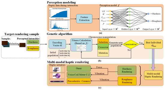
Figure 1.
(a) Perception modeling. BP neural network is used to implement the perception model that establishes the mapping from objective features to perception intensities. (b) Select the target rendering sample. GA generates populations and utilizes the perception model to calculate the fitness of the individual. The best individual is not obtained until termination. (c) is used to control different haptic actuators for multi-modal haptic rendering.
2. Data Collection and Perception Modeling
Data collection is required to build the objective-to-subjective perception model. Firstly, data collection and feature extraction were carried out under specified collection actions. Then, psychophysical experiments for hardness and roughness were performed separately to obtain subjective data. Finally, we exploited the nonlinear fitting ability of BP neural network to establish the perception model f that describes the mapping from objective stimuli features to perception intensities .
2.1. Objective Data Collection and Feature Extraction
Twenty-three samples (S1–S23) were made by combining different substrate materials and textures, for example soft sponge and leather 1 made up sample 1 (S1) in Figure 2. The textures included leather and fabric, and the substrate materials included sponge, EVA (ethylene vinyl acetate) plastic, rubber, and foam to ensure that the samples had a certain degree of difference in hardness and roughness. In this paper, for the properties of hardness and roughness, two interactive actions of pressing and lateral motion are selected for data acquisition [16].
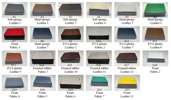
Figure 2.
The twenty-three samples used in this paper.
As shown in Figure 3a, a three-axis accelerometer (Analog Devices ADXL345) is mounted in the front of the wearable fingertip device. A force sensor (Honeywell FSS1500) is mounted at the bottom of the wearable fingertip device. The weight of the wearable fingertip device is 37.2 g. The accelerometer was configured with a dynamic range of ±16 g and 10-bit resolution and connected to the STM32 microcontroller at the wrist over the I2C bus. The force sensor data were obtained with the Analog Digital Converter (ADC, 12 bits) of the microcontroller. We used serial communication to enable the computer to communicate with the STM32 microcontroller to transmit control commands and receive sensory signals. The SensAble Phantom Omni device can sense position, velocity in the x, y, z direction [17]. Displacement data were collected through Omni. Through a guide ball of the Labview interface, the speed of the lateral motion was limited to about 80 mm/s. We collected data for each sample 10 times during the pressing and lateral motion. The collected data were stored in the PC at the acquisition frequency of 500 Hz through Labview platform. Then the force and displacement data were lowpass filtered through a Butterworth filter with a 10 Hz cutoff frequency which was above the normal hand motion bandwidth of 2 Hz to avoid significant delay or attenuation of deliberate human motions [18]. The acceleration data were highpass filtered through a Butterworth filter with a 20 Hz cutoff frequency in order to remove a gravity component and noise [8].
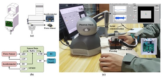
Figure 3.
(a) The schematic diagram of the wearable fingertip device. (b) The block diagram of the STM32 board at the wrist. (c) Haptic data recording interface.
After data collection, we extracted five features related to hardness and roughness in the interation data as vector . In terms of hardness feature extraction, as in [19,20], the global stiffness , and work during the pressing process were extracted, as shown in Figure 4a. In terms of roughness feature extraction, Yoshioka and Culbertson proposed that vibration power has a high correlation with roughness [21,22]. We focused on the acceleration signal of the lateral motion direction of the three-axis acceleration, so the lateral vibration power during the lateral sliding process was extracted. As in [23], we extracted the peak frequency and its amplitude after the FFT of the acceleration signal, as shown in Figure 4b. The means and standard deviations of twenty-three samples’ features are shown in Figure 5.
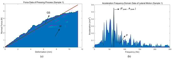
Figure 4.
The interaction data and features of Sample 1 (S1) in the exploring process. (a) Force data and features in pressing process. (b) Acceleration frequency domain data and features during lateral motion.
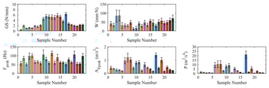
Figure 5.
The means and standard deviations of twenty-three samples’ features.
2.2. Subjective Data Collection
Psychophysical experiments for hardness and roughness were performed separately to obtain subjective data. We recruited 10 participants from Southeast University aged on average 25. All of them were right-handed, and reported having no cutaneous or kinesthetic problems. Two adjective rating experiments were performed on 23 samples using the fingertip device in Figure 3.
Process
Participants wore an eye mask and headphones to shield visual and auditory information from distractions. The samples were presented to the participants in an unordered order. In the first experiment, participants were required to rate the hardness of the samples on a scale of 0–100, where 100 meant “hardest” and 0 meant “softest”. In the second experiment, participants were required to rate the roughness of the samples on a scale of 0–100, where 100 meant “roughest” and 0 meant “smoothest”.
Results
The results of subjective data collection were normalized, as shown in Figure 6. Among the 23 samples, S12 has the hardest hardness score, S1 has the softest score, S7 has the roughest roughness score, and S12 has the smoothest score.
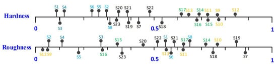
Figure 6.
Hardness, Roughness intensities of the twenty-three samples. The same color indicates that the samples have the same substrate material.
2.3. Perception Modeling
BP neural network was applied using the Levenberg–Marquardt (LM) algorithm to establish the nonlinear perception model. As shown in Figure 1a, we selected features as the input layer parameters, and the hardness and roughness intensities as the output layer parameters. The training was progressed with the MATLAB neural network toolbox. A total of 70% of the total samples were used for training, 15% for validation, and 15% for testing. The training parameter settings are shown in Table 1.

Table 1.
Training parameter settings.
To evaluate the BP model, we use mean square error (MSE) and correlation coefficient (R) as evaluation indicators. Higher prediction accuracy can be represented by smaller MSE value and larger R value. Below are the formulas for MSE and R.
where n is the number of tested instances, is the predicted value estimated by the training network for instance i, and is the target value of instance i. The MSE and R of the BP model is shown in Table 2. As shown in Figure 7, the Hardness MSE of S1 is the smallest among the 23 samples, and the Hardness MSE of S17 is the largest. Among the 23 samples, S12 has the smallest Roughness MSE, and S19 has the largest Roughness MSE.
Table 2.
Evaluation indicators of BP model.
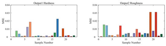
Figure 7.
The Hardness and Roughness MSE for each of the twenty-three samples.
3. Methods
The problem of GA solving can be regarded as the inverse model of the perception model. GA is utilized to obtain the sample’s control characteristics after determining the target sample’s hardness and roughness. We design the fitness function of GA based on the perceptual model and set two physically achievable constraints to limit the fitness calculation. The features of the best individual obtained from GA are transformed into the control features of the target sample.
3.1. Genetic Algorithm
GA was first proposed by John Holland in 1975. The basic idea is that the optimal solution is obtained by simulating the genetic selection process based on evolution theory [24]. The perception model based on BP network is used as the fitness function of GA. We run the algorithm using MATLAB with the settings reported in Table 3. As shown in Figure 1b, GA mainly consists of the following steps:
Table 3.
Settings for the genetic algorithm.
- •
- Chromosome encoding
- •
- Fitness Calculation
- •
- Chromosome Manipulation
- •
- Termination
First, the individual chromosome is encoded as vector (real encoding) as shown in Formula (1) and generates an initial population. The chromosomal genes of the individual are randomly generated within a specific interval that depends on the range of the extracted features in Section 2. Then, GA can evaluate the strength of an individual by the fitness function. The lower the fitness value of the individual, the better the individual. Excellent individuals are likely to be passed on to the next generation.
In order to obtain the features that meet the target sample’s hardness and roughness, we set two physically achievable constraints in the fitness calculation. The constraints punish the fitness value of individuals who do not satisfy the constraints. In order to make the ideal mechanical work done by the GS-controlled actuator not exceed the work done by the pressing process, Formula (4) is used to constrain . In order to ensure that the ideal energy made by the actuator controlled by and does not exceed the energy produced by the vibration of the sliding process, Formula (5) is applied to constrain . The fitness function calculation under constraints is shown in Formula (6).
where H and R are the hardness and roughness intensities of the target sample. and are the two outputs of the BP model after inputting individual chromosome . is the fitness value of chromosome . is the ideal work done by Omni, and is the maximum force 3.3 N at normal position of Omni [25]. is the vibration power at frequency , and is frequency resolution.
In order to generate a new population, it is necessary to perform selection, crossover, and mutation operations on population individuals. The range of chromosome operation to generate new individual is limited by the range of the extracted features in Section 2. When the GA reaches the termination condition, the individual with the best fitness in the current population is selected as the optimal solution. By setting the hardness and roughness intensities of the corresponding samples in GA, the optimal solutions of 23 samples used in this paper are obtained. The results are shown in Figure 8.
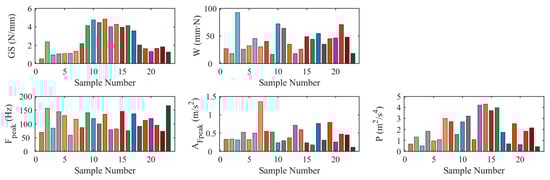
Figure 8.
The best individual chromosome obtained by GA of the twenty-three samples.
3.2. Hardness Rendering Method
GS is used to control the stiffness of Omni for the hardness rendering of the target sample. Since there are samples whose stiffness exceeds the maximum stiffness of Omni (2.3 N/mm), the paper proposes to use the voice coil motor (EAI C-2 tactor) driven by the linear amplifier for the hardness rendering of high-hardness samples. We performed a hardness discrimination experiment to determine the equivalent stiffness of the voice coil motor at different frequency. We collected samples from 10 participants with an average age of 25.
Apparatus
The voice coil motor and one fabricated object that combined with four same springs and a board were placed on a separate digital scale with a distance of about 300 mm, as shown in Figure 9b. There was only one fabricated object. The springs of the fabricated object can be changed. The digital scale’s count was reset to zero before the participants applied force. The operator did not start the voice coil motor until it was observed that the force exerted by the participant remained at around 1N. The driving waveform of the voice coil motor was generated by Labview in real time and output to the linear amplifier through the sound card of the computer at 5 kHz. The amplitude of the waveform remained constant, and the frequency of the waveform can be changed by the operator every 10 Hz between 30 and 120 Hz, with a total of 10 frequency levels. Each frequency level was paired with seven different springs for a total of 70 pairs of parameters. The spring stiffness of the seven springs is shown in Table 4.
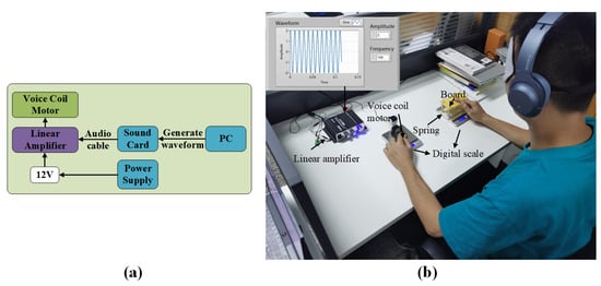
Figure 9.
(a) The block diagram of the voice coil motor control module. (b) Hardness discrimination experiment.
Table 4.
The spring stiffness of seven springs.
Process
The participants were isolated from visual and auditory cues. Firstly, a frequency level of the voice coil motor was randomly selected, and then one of the seven stiffness springs was randomly selected as the springs of the board. The voice coil motor was under the left fingertip, and the board was under the right fingertip. Participants judged whether the spring was stiffer than the voice coil motor stimulus. After completing all stimuli at one frequency level, participants were allowed to rest for 5 minutes. The process was then repeated until all parameter pairs were complete. A total of 700 responses were collected.
Results
The results were analyzed by the Point of Subjective Equality (PSE) [26,27]. PSE is the “subjective equality point”, which means that the value of the subjectively perceived comparison stimulus is the same as the value of the reference stimulus, and the PSE is given by the 50% probability point. Answers from all participants were added together and probabilities were calculated based on the number of times the spring was stiffer than the stimulation of the voice coil motor, fitted with a cumulative Gaussian distribution. The corresponding PSE was calculated for each stimulation level of the voice coil motor. As shown in Figure 10, the PSE values were plotted accordingly to show trends in participants’ responses to increased vibration frequency and fitted using a two-order regression model Formula (7). The formula of the hardness rendering method is given by Formula (8).
where is the normal force, is the maximum stiffness of Omni 2.3 N/mm, Y is the displacement of the Omni y-axis, is the equivalent stiffnes of the voice coil motor, and is the frequency of the voltage applied to the voice coil motor.
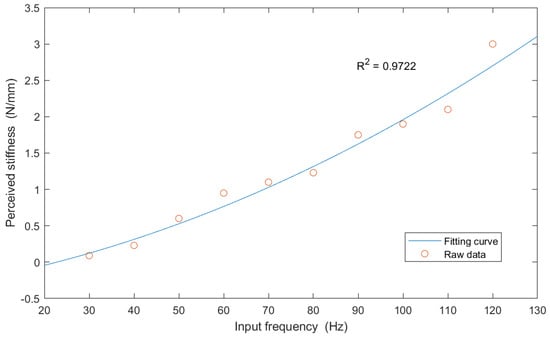
Figure 10.
Fitting curve of equivalent perceived stiffness corresponding to the input frequency of the voice coil motor.
3.3. Roughness Rendering Method
The piezoelectric ceramic (Samsung PHAT423535XX) driven by piezo haptic driver (TI DRV2667) is applied to render roughness. The piezoelectric ceramic was connected to the control module over the I2C bus. We used serial communication to enable the computer to communicate with the control module to transmit control commands. and are used to control the voltage waveform. The piezoelectric ceramic vibrated when the velocity of the x-axis of the Omni exceeded 20 mm/s. In the paper, the surface of sample is approximately defined as a sinusoidal surface with a given wavelength of , as shown in Figure 11. When is constant, the vibration frequency f generated by the surface is proportional to the speed, is regarded as the frequency at speed . When the speed changes, the frequency changes proportionally [28]. The formula of the roughness rendering method is given by Formula (9).
where is the voltage signal applied to the piezoelectric ceramic, is the amplitude of the voltage applied, can obtain the corresponding voltage amplitude of the piezoelectric ceramic at different sample peak frequency and its amplitude in Figure 12, is the lateral velocity 80 mm/s, is the velocity of the x-axis of the Omni, and is the frequency of the piezoelectric ceramic voltage waveform.
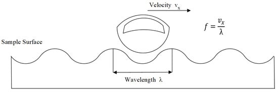
Figure 11.
Definition of surface from using wavelength .
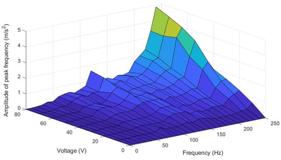
Figure 12.
The acceleration amplitude of the piezoelectric ceramic at different frequency and voltage.
4. Evaluation of Rendering
The rendering features of the target sample can be obtained through Section 3. Omni, voice coil motor, and piezoelectric ceramic are combined to render the hardness and roughness. A total of 8 representative samples (S1, S2, S7, S12, S13, S14, S16, S20) are selected from 23 samples. The realism rating experiment was performed on the 8 samples under three rendering methods. Data analysis is performed on the results of the realism rating experiment.
4.1. Realism Rating Experiment
We recruited 10 participants with an average age of 25 to participate in the realism rating experiment. All of them were right-handed, and reported having no cutaneous or kinesthetic problems. The three rendering methods in the realism rating experiment are shown as follows:
(1) No Roughness: Remove rendering of roughness component. The Omni is used to render the hardness component. The voice coil motor is utilized to render hardness when target rendering sample’s GS exceeds Omni’s maximum rendering stiffness.
(2) No Hardness: Remove rendering of hardness component. The piezoelectric ceramic is used for roughness rendering, and Omni only provides 1N of normal constant force.
(3) All: The hardness and roughness components are displayed together.
Apparatus
As shown in Figure 13c, the participant sat at a table in front of a computer and wore headphones that played white noise to mask outside sounds. The real sample was obscured to prevent the participants from being visually affected by the real sample. The Omni with an attached fingertip device (integrating a voice coil motor and piezoelectric ceramic) was used to render the virtual sample and another Omni handle was utilized to feel the real sample. The weight of the fingertip device is 45.6 g. The voice coil motor driven by the linear amplifier (Figure 9) vibrated when the Omni detected that the participant touched the virtual sample in the virtual interface. The piezoelectric ceramic vibrated when the velocity of the x-axis of the Omni exceeded 20 mm/s.
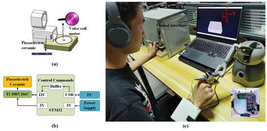
Figure 13.
(a) The schematic diagram of the fingertip device. (b) The block diagram of the piezoelectric ceramic control module. (c) Haptic rendering interface. The participant used Omni with the attached fingertip device to feel the virtual sample and another Omni handle to feel the real sample.
Process
Firstly, participants used the right Omni with the fingertip device to learn how to interact with a virtual sample. Then, the operator provides participants with random real samples to feel. After the participants used left Omni handle to experience the real samples, the operator randomly showed one of the three virtual rendering methods, and each rendering time was within 30 s. Participants were required to use the real sample as a reference to rate the realism of the virtual sample under the three rendering methods on a scale of 0–100, where 100 meant “completely real” and 0 meant “completely unreal”.
4.2. Result
Because the collected data passed the Shapiro–Wilk normality test but not Levene’s homogeneity test, Welch ANOVA was used to compare the means among the three rendering methods [29]. The means differed significantly among the three rendering methods . The Games Howell multiple comparison test was conducted on the Welch ANOVA results. The results revealed statistically significant difference between No Roughness and No Hardness , No Roughness and All , No Hardness and All as shown in Figure 14. The mean ratings were ranked as All (70.86) > No Roughness (57.81) > No Hardness (50.23). The mean rating score for the virtual samples with All haptic rendering was higher than the virtual samples with the removal of the roughness or hardness component. This indicated that the multi-modal haptic rendering is more in line with the feeling of the real sample than the single mode.
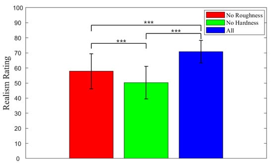
Figure 14.
Comparison of realism ratings across the three rendering methods of the eight samples. Statistically significant differences in realism ratings of the three rendering methods are marked with bars and asterisks (***).
In order to further analyze the effect of removing the roughness or hardness component on the realism rating under each sample, we used the Shapiro–Wilk normality test to verify a normal distribution of the data for each sample. Levene’s homogeneity test was utilized to check the variance homogeneity of the data for each sample. Because the data for each sample passed the Shapiro–Wilk normality test and Levene’s homogeneity test, we performed ANOVA to compare the means among the three rendering methods for each sample. A Tukey–Kramer multiple comparison test was conducted on the ANOVA results. Figure 15 shows the relative importance of matching hardness and roughness for different samples.
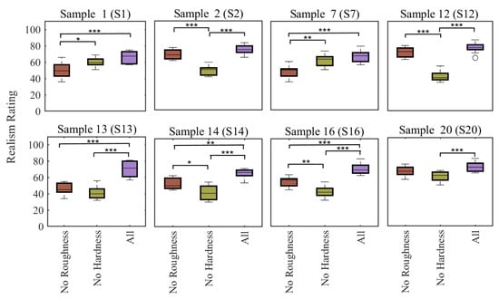
Figure 15.
Comparison of realism ratings across the three rendering methods of each sample. (*** ≡ p ≤ 0.001, ** ≡ p ≤ 0.01, * ≡ p ≤ 0.05).
Realism ratings had statistically significant difference under conditions where a certain rendering component was removed. While some other samples had no statistically significant difference under removing one rendering component. Removing the rendering of the roughness component created statistically significant differences in realism rating between No Roughness and All for five samples: S1 , S7 , S13 , S14 , S16 . Removing the rendering of the hardness component created statistically significant differences in realism rating between No Hardness and All for six samples: S2 , S12 , S13 , S14 , S16 , S20 .
To determine how the realism rating of a virtual sample changes when the roughness or hardness rendering component was removed, the realism ratings of all participants were averaged. Then, we took the same approach as [1] and treated the change in the realism rating as a function of the features (obtained by GA). The difference percentage was calculated as follows:
where is the average realism rating when all rendering components were displayed, and is the average realism rating when roughness or hardness component was removed. A multiple regression analysis was conducted to analyze the factors influencing the realism rating of virtual samples due to the removal of the roughness or the hardness component (Table 5 and Table 6).
Table 5.
Factors related to the realism rating of the removal of roughness (multivariate analysis).
Table 6.
Factors related to the realism rating of the removal of hardness (multivariate analysis).
5. Discussion
By analyzing the relationship between the features obtained by GA and the perceptual intensities (hardness, roughness) of real samples, we verified whether the features capture the perceptual dimensions of real samples. The relationship between the features obtained by GA and the real hardness and roughness of the object was obtained by Spearman correlation analysis in Figure 16. The results showed that the features capture the hardness and roughness of objects. The study provided valuable guidance on the importance of hardness and roughness rendering for the realism of virtual samples by evaluating sample realism changes under removing the hardness or roughness rendering component.
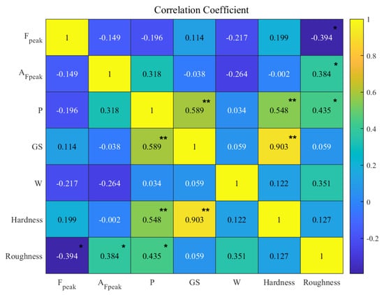
Figure 16.
Correlation between features and hardness, roughness (** ≡ p ≤ 0.01, * ≡ p ≤ 0.05).
5.1. Correlation Analysis
The results of correlation showed that there was a significant positive correlation between GS and Hardness , which indicated that larger GS would bring greater hardness perception. There was a significant positive correlation between P and Hardness , between P and Roughness , which was analyzed due to the greater vibration intensity transmitted by tool interaction on harder or rougher objects. There was a negative correlation between and Roughness . Under constant interaction speed, we inferred that the larger the , the smoother an object was. There was a positive correlation between and Roughness . In the case of constant interaction speed, we inferred that the larger the , the rougher an object was.
5.2. Factors Related to the Realism Rating of the Removal of Roughness or Hardness Component
When the roughness component was removed, and had a significant effect on the percent difference in realism rating. The explanatory power was 84.2% as shown by in Table 5. The results showed that was highly negatively correlated with the percent difference in realism rating, and was highly correlated with the percent difference in realism rating. The results suggested that roughness rendering was more important for samples with low and high when interacting with the samples. The Roughness rating and were moderately negatively correlated. The Roughness rating and were moderately correlated. The results indicated that roughness rendering was more important for rougher samples. For some smooth samples, roughness rendering may not even be required.
When the hardness component was removed, GS significantly affected the percent difference in realism rating. The explanatory power was 95.2% as shown by in Table 6. The results showed that GS was highly negatively correlated with the percent difference in realism rating. The results suggested hardness rendering was more essential for samples with higher GS. The Hardness rating and GS were highly correlated. The results indicated that hardness rendering was more important for harder samples, and it may provide a small constant force for the rendering of some soft samples.
6. Conclusions
In this paper, we propose a multi-modal haptic rendering algorithm based on GA and BP neural network to display the multiple perceptual intensities of the object, which generate force and vibration stimuli according to the target sample’s hardness and roughness. The Omni and voice coil motor are applied to render the hardness of the object, and the piezoelectric ceramic is utilized to render the roughness. Finally, we performed a realism rating experiment in which subjects compared real samples with virtual samples under multi-modal rendering or removing the hardness or roughness component. The results proved that multi-modal rendering improves realism. Based on the work, our method can be applied to render objects in more perceptual dimensions, not only limited to hardness and roughness of the paper. It has important implications for multi-modal haptic rendering.
There are also some limitations in our work. We only performed realistic evaluation experiments for the existing 8 real samples. Since our samples are selected from 23 samples and cannot cover the haptic properties of all sample categories, the type of rendering samples has certain limitations. Through the method in the paper, control features can also be obtained for virtual samples that do not exist corresponding to real samples among our 23 samples, but the realism of such virtual samples remains to be evaluated. To better render virtual objects, other features and actuators may be tried, which is the direction of our future work.
Author Contributions
Conceptualization, Y.L. and J.W.; Data curation, Y.L. and F.W.; Formal analysis, Y.L., F.W. and L.T.; Funding acquisition, J.W.; Investigation, Y.L. and F.W.; Methodology, Y.L. and J.W.; Project administration, J.W.; Resources, J.W.; Software, F.W.; Validation, F.W. and L.T.; Visualization, Y.L.; Writing—original draft, Y.L. and L.T.; Writing—review and editing, Y.L. and J.W. All authors have read and agreed to the published version of the manuscript.
Funding
This research was funded by National Key R&D Program of China under grant 2018AAA0103001 and National Natural Science Foundation of China under grant 62073073.
Institutional Review Board Statement
Not applicable.
Data Availability Statement
Not applicable.
Acknowledgments
This research was supported by National Natural Science Foundation of China under grant 62073073, Jiangsu Key Laboratory for Remote Measurement and Control.
Conflicts of Interest
The authors declare no conflict of interest.
References
- Culbertson, H.; Kuchenbecker, K.J. Importance of matching physical friction, hardness, and texture in creating realistic haptic virtual surfaces. IEEE Trans. Haptics 2016, 10, 63–74. [Google Scholar] [CrossRef] [PubMed]
- Tiest, W.M.B. Tactual perception of material properties. Vision Res. 2010, 50, 2775–2782. [Google Scholar] [CrossRef] [PubMed]
- Abiri, A. Investigation of Multi-Modal Haptic Feedback Systems for Robotic Surgery; University of California: Los Angeles, CA, USA, 2017. [Google Scholar]
- Oo, S.S.; Hanif, N.H.H.M.; Elamvazuthi, I. Closed-loop force control for haptic simulation: Sensory mode interaction. In Proceedings of the 2009 Innovative Technologies in Intelligent Systems and Industrial Applications, Kuala Lumpur, Malaysia, 25–26 July 2009; pp. 96–100. [Google Scholar]
- Okamura, A.M.; Cutkosky, M.R.; Dennerlein, J.T. Reality-based models for vibration feedback in virtual environments. IEEE/ASME Trans. Mechatronics 2001, 6, 245–252. [Google Scholar] [CrossRef]
- Bergmann Tiest, W.M.; Kappers, A.M. Kinaesthetic and cutaneous contributions to the perception of compressibility. In Proceedings of the International Conference on Human Haptic Sensing and Touch Enabled Computer Applications, Madrid, Spain, 11–13 June 2008; Springer: Berlin/Heidelberg, Germany, 2008; pp. 255–264. [Google Scholar]
- Culbertson, H.; Unwin, J.; Kuchenbecker, K.J. Modeling and rendering realistic textures from unconstrained tool-surface interactions. IEEE Trans. Haptics 2014, 7, 381–393. [Google Scholar] [CrossRef] [PubMed]
- Abdulali, A.; Jeon, S. Data-driven rendering of anisotropic haptic textures. In Proceedings of the International AsiaHaptics Conference, Chiba, Japan, 29 November–1 December 2016; Springer: Berlin/Heidelberg, Germany, 2016; pp. 401–407. [Google Scholar]
- Osgouei, R.H.; Shin, S.; Kim, J.R.; Choi, S. An inverse neural network model for data-driven texture rendering on electrovibration display. In Proceedings of the 2018 IEEE Haptics Symposium (HAPTICS), San Francisco, CA, USA, 25–28 March 2018; pp. 270–277. [Google Scholar]
- Osgouei, R.H.; Kim, J.R.; Choi, S. Data-driven texture modeling and rendering on electrovibration display. IEEE Trans. Haptics 2019, 13, 298–311. [Google Scholar] [CrossRef] [PubMed]
- Alma, U.A.; Altinsoy, E. Perceived roughness of band-limited noise, single, and multiple sinusoids compared to recorded vibration. In Proceedings of the 2019 IEEE World Haptics Conference (WHC), Tokyo, Japan, 9–12 July 2019; pp. 337–342. [Google Scholar]
- Xia, P. New advances for haptic rendering: State of the art. Vis. Comput. 2018, 34, 271–287. [Google Scholar] [CrossRef]
- Gao, Y.; Hendricks, L.A.; Kuchenbecker, K.J.; Darrell, T. Deep learning for tactile understanding from visual and haptic data. In Proceedings of the 2016 IEEE International Conference on Robotics and Automation (ICRA), Stockholm, Sweden, 16–21 May 2016; pp. 536–543. [Google Scholar]
- Ouyang, Q.; Wu, J.; Shao, Z.; Chen, D.; Bisley, J.W. A simplified model for simulating population responses of tactile afferents and receptors in the skin. IEEE Trans. Biomed. Eng. 2020, 68, 556–567. [Google Scholar] [CrossRef] [PubMed]
- Li, J.; Cheng, J.h.; Shi, J.y.; Huang, F. Brief introduction of back propagation (BP) neural network algorithm and its improvement. In Advances in Computer Science and Information Engineering; Springer: Berlin/Heidelberg, Germany, 2012; pp. 553–558. [Google Scholar]
- Lederman, S.J.; Klatzky, R.L. Extracting object properties through haptic exploration. Acta Psychol. 1993, 84, 29–40. [Google Scholar] [CrossRef] [PubMed]
- McMahan, W.C. Providing Haptic Perception to Telerobotic Systems via Tactile Acceleration Signals; University of Pennsylvania: Philadelphia, PA, USA, 2013. [Google Scholar]
- Culbertson, H.; Romano, J.M.; Castillo, P.; Mintz, M.; Kuchenbecker, K.J. Refined methods for creating realistic haptic virtual textures from tool-mediated contact acceleration data. In Proceedings of the 2012 IEEE Haptics Symposium (HAPTICS), Vancouver, BC, Canada, 4–7 March 2012; pp. 385–391. [Google Scholar]
- Piovarči, M.; Levin, D.I.; Rebello, J.; Chen, D.; Ďurikovič, R.; Pfister, H.; Matusik, W.; Didyk, P. An interaction-aware, perceptual model for non-linear elastic objects. ACM Trans. Graph. (TOG) 2016, 35, 1–13. [Google Scholar] [CrossRef]
- Shao, Z.; Cao, Z.; He, C.; Ouyang, Q.; Wu, J. Perceptual model for compliance in ineraction with compliant objects with rigid surface. In Proceedings of the 2020 IEEE International Conference on Power, Intelligent Computing and Systems (ICPICS), Shenyang, China, 28–30 July 2020; pp. 246–252. [Google Scholar]
- Yoshioka, T.; Bensmaia, S.J.; Craig, J.C.; Hsiao, S.S. Texture perception through direct and indirect touch: An analysis of perceptual space for tactile textures in two modes of exploration. Somatosens. Mot. Res. 2007, 24, 53–70. [Google Scholar] [CrossRef] [PubMed]
- Vardar, Y.; Wallraven, C.; Kuchenbecker, K.J. Fingertip interaction metrics correlate with visual and haptic perception of real surfaces. In Proceedings of the 2019 IEEE World Haptics Conference (WHC), Tokyo, Japan, 9–12 July 2019; pp. 395–400. [Google Scholar]
- Fiedler, T. A novel texture rendering approach for electrostatic displays. In Proceedings of the International Workshop on Haptic and Audio Interaction Design-HAID2019, Lille, France, 13–15 March 2019. [Google Scholar]
- Sampson, J.R. Adaptation in Natural and Artificial Systems (John H. Holland); Society for Industrial and Applied Mathematics: Philadelphia, PA, USA, 1976. [Google Scholar]
- Song, Z.; Guo, S.; Yazid, M. Development of a potential system for upper limb rehabilitation training based on virtual reality. In Proceedings of the 2011 4th International Conference on Human System Interactions, HSI 2011, Yokohama, Japan, 19–21 May 2011; pp. 352–356. [Google Scholar]
- Lécuyer, A.; Coquillart, S.; Kheddar, A.; Richard, P.; Coiffet, P. Pseudo-haptic feedback: Can isometric input devices simulate force feedback? In Proceedings of the IEEE Virtual Reality 2000 (Cat. No. 00CB37048), New Brunswick, NJ, USA, 18–22 March 2000; pp. 83–90. [Google Scholar]
- Porquis, L.B.; Konyo, M.; Tadokoro, S. Representation of softness sensation using vibrotactile stimuli under amplitude control. In Proceedings of the 2011 IEEE International Conference on Robotics and Automation, Shanghai, China, 9–13 May 2011; pp. 1380–1385. [Google Scholar]
- Konyo, M.; Tadokoro, S.; Yoshida, A.; Saiwaki, N. A tactile synthesis method using multiple frequency vibrations for representing virtual touch. In Proceedings of the 2005 IEEE/RSJ International Conference on Intelligent Robots and Systems, Edmonton, AB, Canada, 2–6 August 2005; pp. 3965–3971. [Google Scholar]
- Pacchierotti, C.; Abayazid, M.; Misra, S.; Prattichizzo, D. Teleoperation of steerable flexible needles by combining kinesthetic and vibratory feedback. IEEE Trans. Haptics 2014, 7, 551–556. [Google Scholar] [CrossRef] [PubMed]


Publisher’s Note: MDPI stays neutral with regard to jurisdictional claims in published maps and institutional affiliations. |
© 2022 by the authors. Licensee MDPI, Basel, Switzerland. This article is an open access article distributed under the terms and conditions of the Creative Commons Attribution (CC BY) license (https://creativecommons.org/licenses/by/4.0/).