Communication

Novel Nonlinear High Order Technologies for Damage Diagnosis of Complex Assets

1
Faculty of Electrical Engineering, Gdynia Maritime University, 81-255 Gdynia, Poland
2
School of Computing and Engineering, University of Huddersfield, Huddersfield HD1 3DH, UK
*
Author to whom correspondence should be addressed.
Electronics 2022, 11(23), 3885; https://doi.org/10.3390/electronics11233885
Submission received: 13 October 2022 / Revised: 11 November 2022 / Accepted: 15 November 2022 / Published: 24 November 2022

Abstract

:
For the first time worldwide, innovative techniques, generic non-linear higher-order unnormalized cross-correlations of spectral moduli, for the diagnosis of complex assets, are proposed. The normalization of the proposed techniques is based on the absolute central moments, that have been proposed and widely investigated in mathematical works. The existing higher-order, cross-covariances of complex spectral components are not sufficiently effective. The novel technology is comprehensively experimentally validated for induction motor bearing diagnosis via motor current signals. Experimental results, provided by the proposed technique, confirmed high overall probabilities of correct diagnoses for bearings at early stages of damage development. The proposed diagnosis technology is compared with existing diagnosis technology, based on the triple cross-covariance of complex spectral components.

1. Introduction

Induction motors (IMs) are widely employed in various industrial, military, and civil applications. Electric vehicles, gearmotors, and pumps are examples of a broad scope of IM use. Most IMs are required to operate uninterrupted for a long period. That is why a proper condition monitoring and maintenance are a must in industrial applications of motors, gearmotors, and other structures [1,2,3,4,5,6,7,8,9,10,11,12,13,14,15,16,17,18,19,20,21,22,23,24,25,26,27,28,29,30,31,32,33,34,35,36]. Publication [7] presents very wide and comprehensive state-of-the-art IM faults, detection, and diagnosis. Proper fault detection and fault isolation of key components is crucial for continuity of IM operation. Among the most common elements, susceptible to damage in an IM, are its bearings, accounting for 42% of all failures [7]. That is why their effective diagnosis is of utmost importance. The ability to diagnose bearing conditions is the subject of continuous research and development [1,3,5,6,8,20,21,23,25,26,27,28,29].
For industrial bearings diagnosis, vibration-based methods are still the most used. However, they require the installation of accelerometers on the engine, making these methods invasive, inconvenient, and costly. Vibration analysis is a well-proven method, that has been used for a long-time to detect bearing damage [5,25,26,27,28,33,34,35,36]. Vibration methods are still being improved, mainly in terms of signal processing. In [25], a method, enabling diagnostics in conditions of variable rotational speed, is presented. Paper [26] presents a solution, based on the spectral kurtosis and the wavelet transform.
In the recent years, motor current signature analysis (MCSA) is the subject of much research; it becomes a convenient alternative to vibration-based methods for IM diagnosis. This non-invasive method allows to significantly reduce the cost of diagnosis as it does not require installation of expensive vibration sensors on a motor. MCSA does not require a direct access to a diagnosed motor; only access to a power supply line of a motor is needed. Motor current signals are widely used for detecting electrical and mechanical faults in motors and coupled gearboxes. Early diagnosis of bearing faults via MCSA is a difficult task due to a low signal/ noise ratio (SNR) of spectral components, carrying diagnostic information [4,5,6,7,8,10,19,20,21,22,24,29]. Changes in the temporal shape of current waveforms, caused by bearing damage, are practically imperceptible, and therefore most of MCSA methods use current spectral presentations. Due to a poor SNR of bearing diagnostic components in the current spectrum, many spectral harmonics of a different nature may match in frequency areas. Therefore, it is crucial to estimate frequencies of bearing defect characteristic components, with a high accuracy, to track those components in time—frequency domain. Precise rotational speed estimations of a motor rotor are needed to estimate these frequencies. Rotor speed can be estimated via current spectrum and rotor slot harmonics (RSH) with high precision. A rotor speed estimation method, based on RSH frequency demodulation, is introduced in [30]; this method gives accurate results for both transient and steady-state motor operations.
Models for frequencies of current characteristic spectral components have been improved over time. Works [8,9] have shown that some of the previous MCSA solutions, e.g., [4], are based on an incomplete model for characteristic frequency estimations. In [9], changes of torque, caused by bearing damage, are taken into account. It has been shown that oscillations of torque, have an essential influence on characteristic frequencies. In cases of inner race or rolling elements damage, characteristic frequencies are different, when compared with earlier research works, e.g., [4]. In [8], a dynamic model of a rotor with damaged bearings is presented in order to numerically simulate an air gap. The current modelling is built on a magnetic circuit.
A different approach to IM bearing condition monitoring, presented in [5,20], proposes determining characteristic frequencies via vibration methods. Spectral components, identified via vibration signal envelope analysis, are tracked in current spectrum, and changes in their amplitude are used for bearing diagnosis.
In [21] a new Fault-excited Harmonic Distortion diagnostic indicator is proposed. The developed IM model showed a dependency between the proposed diagnostic indicator and bearing fault severity. However, this method was tested only for one outer race defect for a specific type of IM. Other mathematical expressions for this method are needed for other types of IM. The model, presented in [21], does not take into account saturation of the motor core, and only radial eccentricities related to a damage, are considered.
For increasing bearing damage detection efficiency via MCSA, new, more effective signal processing solutions are sought. In recent research works on this topic, the wavelet transform [6,9,31,32,33,34,35,36], the higher-order spectral techniques [1,3,22,24], and the spectral kurtosis [26,28] are used.
In [6], the continuous wavelet transform is applied via MCSA to detect damage in bearing localized in motor load, and not in the motor. It is not an easy task, because such damage does not affect the air gap of tested motors; only changes of a motor load momentum can affect motor current. For this reason, the characteristic spectral components in the motor current spectrum are barely detectable via methods, based on the current spectrum [6].
The higher-order spectral techniques are used in [1,3,22,24] for MCSA to detect IM damage. These techniques give an insight into the interactions of spectral components. It has been shown that it is possible not only to detect early fault, but also indicate a fault severity.
In [23], an MCSA method, that involves instantaneous frequency analysis, was proposed [19] considers motor bearing diagnosis. For light load conditions, MCSA methods mostly fail in detecting this type of damage, due to poor SNR. The proposed method was tested on a small number of bearing faults, and only outer race defects were considered in this research.
Another way of dealing with a poor SNR of bearing diagnostic components in motor current signal is the Park vector approach. Approach advantage is an essential enhancement of components, carrying diagnostic information. Then, various sophisticated methods of signal processing [19,26,29] can be used for component fault detection. This approach is used for detection of bearing faults [19,20,29,37,38,39,40,41], as well as other faults of IMs, such as broken rotor bar [42,43,44,45,46,47,48] and stator winding faults [49,50,51,52].
The main novelty proposed here is the generic, non-linear, high-order technologies for damage diagnosis and the higher-order, unnormalized, cross-correlations of spectral moduli for steady and non-steady functioning of complex systems.
Research carried here shows a very essential advantage of the proposed technologies: they provide an effective damage diagnosis for any damage related spectral components, including components that do not follow bicoherence/tricoherence frequency rules.
Other innovations of the presented research:
  • technology validations via extensive experiments
  • comparison of the proposed technology and the cross-covariance technology, based on t complex spectra
The aims of the research are to:
  • propose new damage diagnosis technologies, cross-correlations of moduli for steady and non-steady functioning of complex systems,
  • perform technology testing via extensive experiments using motor current signal processing and,
  • perform technology comparisons between triple cross-covariance technologies, based on complex spectra, using motor current signature analysis.

2. The Cross-Correlations of Spectral Moduli

Unnormalized cross-correlations of spectral moduli (UCCSM) of order n are proposed here for the first time worldwide. The first step in the estimation of UCCSM is to divide signal into time segments. The second step is to perform the selected frequency transform or time-frequency transform for each time segment. The third step is to estimate moduli of the spectral components at the selected characteristic frequencies, or at the selected characteristic time-frequency points. The final step is to estimate the unnormalized cross-correlation for each segment and to average these cross-correlations over all segments. The normalized cross-correlations (CCSM) of n moduli of spectral components are estimated via Equation (1):
CCSM ( f 1 , f 2 , , f n , t ) = j = 1 I [ ( mY f 1 j ( t ) ) ( mY f 2 j ( t ) ) ( mY f n j ( t ) ) ] j = 1 I [ | mY f 1 j ( t ) mY f 1 ( t ) ¯ | n ] n   j = 1 I [ | mY f 2 j ( t ) mY f 2 ( t ) ¯ | n ] n j = 1 I [ | mY f n j ( t ) mY f n ( t ) ¯ | n ] n  
where I is segment number, mY f n j is the modulus related to any complex time-frequency transform, or any complex frequency transform of time segment j for frequency f n .
Normally, normalization of higher-order correlations of random variables is based on the absolute central moments of order n, proposed and widely investigated in many mathematical works, e.g., [53,54,55,56,57]. Another normalization [1,2,3] is also possible.
The main dissimilarity between the proposed technologies (1), the higher-order spectral cross-covariance technologies in refs [1,2,3], and the classical higher-order spectra [58] is that the proposed cross-correlations are estimated for the moduli of complex frequency transforms and complex time-frequency transforms. The proposed use of complex transform moduli for higher-order spectral techniques is non-traditional, as traditionally e.g., [1,2,3,7,16,18,22,24,27,58,59], in applications by all known authors of higher-order spectral techniques and the complex spectral components (not moduli of complex spectral components) are used.
The main reason that complex spectral components are used is that phase information, related to these components, could be employed for diagnostic purposes. This reason is fully justifiable for pure complex exponential signals. However, characteristic time domain signals, that are involved/important in vibration fault diagnosis and in diagnosis via MCSA, are, normally, not pure complex exponential signals. These signals are narrowband random signals with random phases. It is shown here, that for current narrowband signals, it is more efficient to employ the higher-order spectral technologies, based on moduli of complex spectral components. The employment of moduli of complex transforms is an essential novel feature of the technologies, which depend only on moduli of the selected complex characteristic components, and are not dependent on the phase spectra of the selected characteristic spectral components.
It is known [60,61], that the phase spectra of single characteristic spectral components are important for fault diagnosis. However, as the proposed technologies do not employ single characteristic spectral components, but employ, simultaneously, multiple characteristic spectral components, it is shown below, via experimental trials, that it is more beneficial to exclude from consideration the phase spectra of these spectral components.
The particular uses of the proposed technology (1) are the cross-correlation of spectral moduli of order 3 (CCSM3) and the cross-correlation of spectral moduli of order 4 (CCSM4), expressed as follows:
CCSM 3 ( f 1 , f 2 , f 3 , t ) = j = 1 I [ ( mY f 1 j ( t ) ) ( mY f 2 j ( t ) ) ( mY f 3 j ( t ) ) ] j = 1 I [ | mY f 1 j ( t ) mY f 1 ( t ) ¯ | 3 ] 3   j = 1 I [ | mY f 2 j ( t ) mY f 2 ( t ) ¯ | 3 ] 3   j = 1 I [ | mY f 3 j ( t ) mY f 3 ( t ) ¯ | 3 ] 3  
CCSM 4 ( f 1 , f 2 , f 3 , f 4 , t ) = j = 1 I [ ( mY f 1 j ( t ) ) ( mY f 2 j ( t ) ) ( mY f 3 j ( t ) ) ( mY f 4 j ( t ) ) ] j = 1 I [ | mY f 1 j ( t ) mY f 1 ( t ) ¯ | 4 ] 4   j = 1 I [ | mY f 2 j ( t ) mY f 2 ( t ) ¯ | 4 ] 4   j = 1 I [ | mY f 3 j ( t ) mY f 3 ( t ) ¯ | 4 ] 4 j = 1 I [ | mY f 4 j ( t ) mY f 4 ( t ) ¯ | 4 ] 4
The proposed technologies are applicable for steady signals, related to steady functioning of systems, by using spectral moduli of complex frequency transforms and real frequency transforms (e.g., Hartley distribution, the cosine transform, etc.) for (1)–(3). If frequency transforms are employed, the CCSM technologies are not time-dependant. It is proposed that further novel technologies could be used for non-steady functioning of systems (e. g. machinery start-up and speed variation), via the employment of moduli of complex time-frequency transforms [32,33,34,62,63], and real time-frequency transforms (e.g., the Wigner distribution, etc.) for Equations (1)–(3). If time-frequency transforms are employed, the CCSM technologies are time-dependant.
The importance of the technologies is that they estimate cross-correlations between moduli of frequency components. Moduli of frequency components that appear due to faults are correlated.
The main limitations of the proposed technologies are the same, as the limitations of higher-order spectral technologies, as follows:
  • a difficulty of a visual representation of the CCSM for orders greater than 4
  • a computation complexity
  • technologies are becoming non-effective at an excessive level of interference
However, it is known [58] that the higher-order spectral technologies, including the proposed technologies, are more “immune” to an excessive level of interference, than second order technologies.
Let us investigate the CCSM3 for local bearing damage diagnosis via MCSA. The fundamental frequency of the shaft rotation f r and the fundamental frequency of the motor supply current f g are estimated from the obtained motor current spectrum for every time segment of a time domain current signal. It is important to track the frequencies for each time segment to cover possible fluctuations of bearing defect frequencies and the supply frequency. The fundamental frequency of the shaft rotation f r is obtained through RSH frequency estimation and information of motor construction, as described in [30,42], as follows:
f f = f RSH ± f g k · N R
where f RSH is the RSH frequency, f g is the supply grid frequency, f r is the fundamental rotation frequency, k is the rotor bar harmonic number, and N R is the number of rotor bars.
Values of the mentioned frequencies are needed to estimate the frequency specifics of the bearing damage. Next, modulus values from complex spectra, for three spectral components of the selected characteristic frequencies, are obtained for every time segment. The next step is to calculate the Equation (2) for CCSM3 estimation. The last step is to calculate the mean value of CCSM3 for three phases of the IM current.
The number of operations for CCSM3 technology could be estimated as follows. Considering a conventional method of CCSM3 estimation, the main method for estimation of CCSM3 is the direct method [58,59]. Extension of this method to CCSM4 or to any higher CCSM order can be made easily. Considering the direct method of estimation of the numerator of CCSM3 (as estimation of the denominator of the CCSM3 is a computationally easy task) for one diagnostic feature, the following steps should be employed:
  • segmentation of current data into K non-overlapped segments of N samples each
  • estimation of DFT coefficients for each segment
  • calculation of CCSM3 estimates for all segments via multiplications of moduli of the selected DFT coefficients, and average these estimates over K segments
Number of multiplication operations for the estimation of DFT for each segment is Nlog 2 N and the number of addition operations for estimation of DFT for each segment is 2 Nlog 2 N .
Finally, ignoring a small number of addition operations, for the averaging of the CCSM3 over K segments, and a small number of multiplication operations, for obtaining the CCSM3 for each segment, the total number of multiplication operations for K segments is K × Nlog 2 N , and the total number of addition operations for K segments is K × Nlog 2 N .
The two frequencies specific for bearing damage are defined with the Formulas (5) and (6) [1,7,25]:
f out = ( 1 B d P d cos α ) N b = FCC o · f r
f in = 1 2 f r ( 1 + B d P d cos α ) N b = FCC i · f r
where f out is the outer race damage frequency, f in is the inner race damage frequency, f r is the frequency of IM shaft oscillation, N b is the number of rolling elements in the bearing, B d is the diameter of the rolling elements in the bearing, P d is the pitch diameter of a bearing and α is the angle of thrust. FCC o is the fault specific coefficient of the outer race and FCC i is the fault specific coefficient of the inner race.
Coefficients FCC i and FCC o , used in this research, are received from SKF (UK).

3. Experimental Setup and Technology Validation

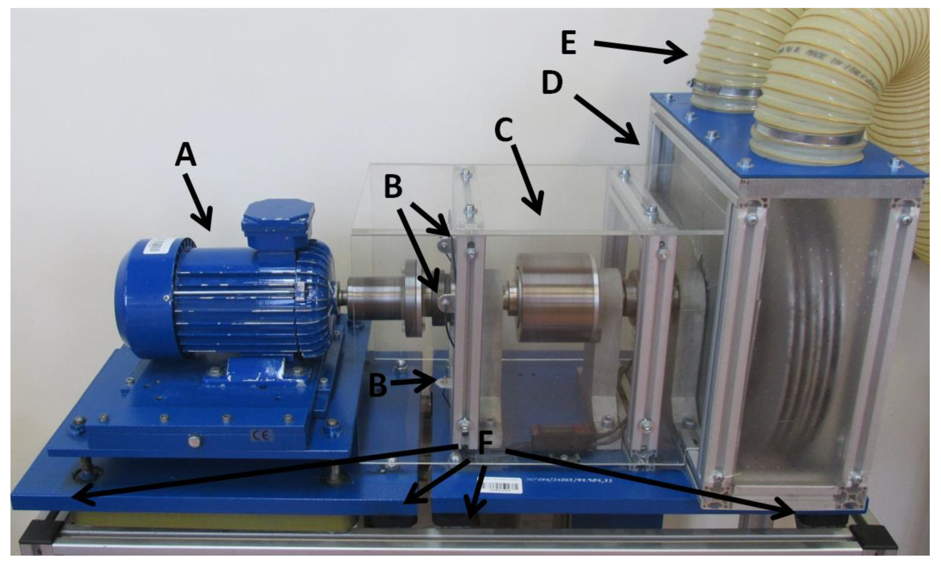
3.1. Setup for Experimental Technology Validation

The test rig, used for experimental technology validation, is presented in Figure 1. Its use is described in detail in [1]. Pointer A shows the IM used in this experiment, pointer B indicates the laser sensors used for shaft alignment, pointer C indicates the magnetic coupling, pointer D shows the electromagnetic brake, pointer E shows the hoses which provide the air for the brake cooling, and pointer F shows the pads used to isolate the test rig form external vibration. The IM in this experiment was powered by the national 50 Hz three phase electrical power grid.
The IM current signal was recorded via a data acquisition system with the use of a specially designed transducer and a 24 bits DAQ system. In general, the main parameters required for a suitable performance of a data acquisition system for CCSM, are as follows: 3 channel differential inputs for three phases, a −120 dB, channel cross-talk, 24-bit conversion, a total harmonic distortion of 0.5%, attenuation of an anti-aliasing filter in the transition band is 100 dB/oct, and a current sensor that is a split-core current transformer, with galvanic separation between the primary circuit (power) and the secondary circuit (data capture).
All IM currents processed in this experiment were recorded for IM, with 6204C3 Koyo bearings. Construction of the bearing, and the absence of the seals, allowed for an easy disassembly of the bearings for damage introduction.
IM current recordings were done for 8 bearings, 4 pristine bearings, and 4 bearings with different types of damage. The close-up photos of the introduced bearing faults are shown in Figure 2. All damages introduced were small local faults, created to simulate bearing damage which had not yet developed; a detailed description of each damage introduced is listed in Table 1. The pristine bearings are labelled as p1, p2, p3, and p4; a pristine bearing is shown in Figure 3.
To achieve effective fault diagnosis results, digital signal processing of the recorded IM current was performed. The IM current signals are recorded for 65 s of an uninterrupted IM work. The Blackman time window was used for each 5 s time segment of the signal, recorded at 65.536 kHz sampling frequency. Technical requirements of the computer used for numerical estimation of CCSM technologies were: Windows 7 or later version, 8 GB of RAM, 3.4 GB of SSD space for MATLAB, a processing speed of 3.4 GHz or higher, a latency of 100 ms, an internal hard-drive speed of 50 MB/s or higher, a bus speed of 5GT/s or higher.
Current data, mentioned above (i.e., segment size is 5 s, number of segments is 13, 0% segment overlapping, sampling frequency is 65.536 kHz), were processed via a PC with Intel Core i7-2600 CPU and 8 GB of RAM, with a computation time of 2 s for one CCSM3 diagnostic feature. If the CCSM3 algorithm software was organised using the calculation of CCSM3 during sample intervals, then the CCSM3 feature could be estimated in “real time”.
Signals are recorded for the four undamaged bearings and for the four counterpart damaged bearings. The four pairs are split into two cases:
  • two inner race damaged bearings vs. two undamaged bearings
  • two outer race damaged bearings vs. two undamaged bearings
Each case was analysed separately. The recorded signals were processed via the proposed CCSM3. Using the above methodology (from Section 2) for estimation of the total number of operations for the calculation of the numerator of the CCSM3, the number of multiplication operations and number of addition operations are 78,040,269 and 156,080,538, respectively, for the processing parameters employed here for experimental trials: segment size is 5 s, the number of segments is 13, the sampling frequency is 65.536 kHz, and the segment overlap is 0%. The total number of operations for calculation of the numerator of CCSM3 is 234120807. The total number of operations, for calculation of CCSM3, that is estimated via Matlab socFunctionAnalyzer, is 310778788, for the above-mentioned processing parameters.
The estimates of the overall probability of correct fault diagnosis are defined by Equation (7):
P t = fN + hN fNt + hNt
where fN is the number of correctly diagnosed bearings with damage, hN is the number of correctly diagnosed healthy bearings, fNt is the total number of diagnoses carried for bearings with damage, and hNt is the total number of diagnoses carried for healthy bearings. The Fisher criterion is defined by Equation (8):
FCr = | am 1 am 2 | 2 σ 1 2 + σ 2 2
where am 1 is the average value of diagnostic features for healthy bearings, am 2 is the average value of diagnostic features for bearings with fault, σ 1 2 is the squared standard deviation of diagnostic features for healthy bearings, and σ 2 2 is the squared standard deviation of diagnostic features for bearings with fault. The overall probability of correct fault diagnosis, Equation (7), and the Fisher criteria, Equation (8), are used to evaluate the quality of diagnosis via the proposed technology.
To diagnose healthy and faulty bearings, a one-dimensional decision-making threshold-based rule was used. The Bayes rule was implemented for this task. If the CCSM diagnostic feature was more than the Bayes based threshold, a damaged diagnosis was given; if the CCSM diagnostic feature was less than the Bayes based threshold, an undamaged diagnosis was given. For multi-class fault identification, more complicated decision-making rules, based on machine learning, would be employed. For each CCSM3, 51 diagnostic features for each bearing were estimated. Time segment overlapping, from 0% to 50%, with a 1% step were used for these estimations. Values of 204 diagnostic features were used for the estimation of the overall probabilities of the true diagnostics and the Fisher criteria.

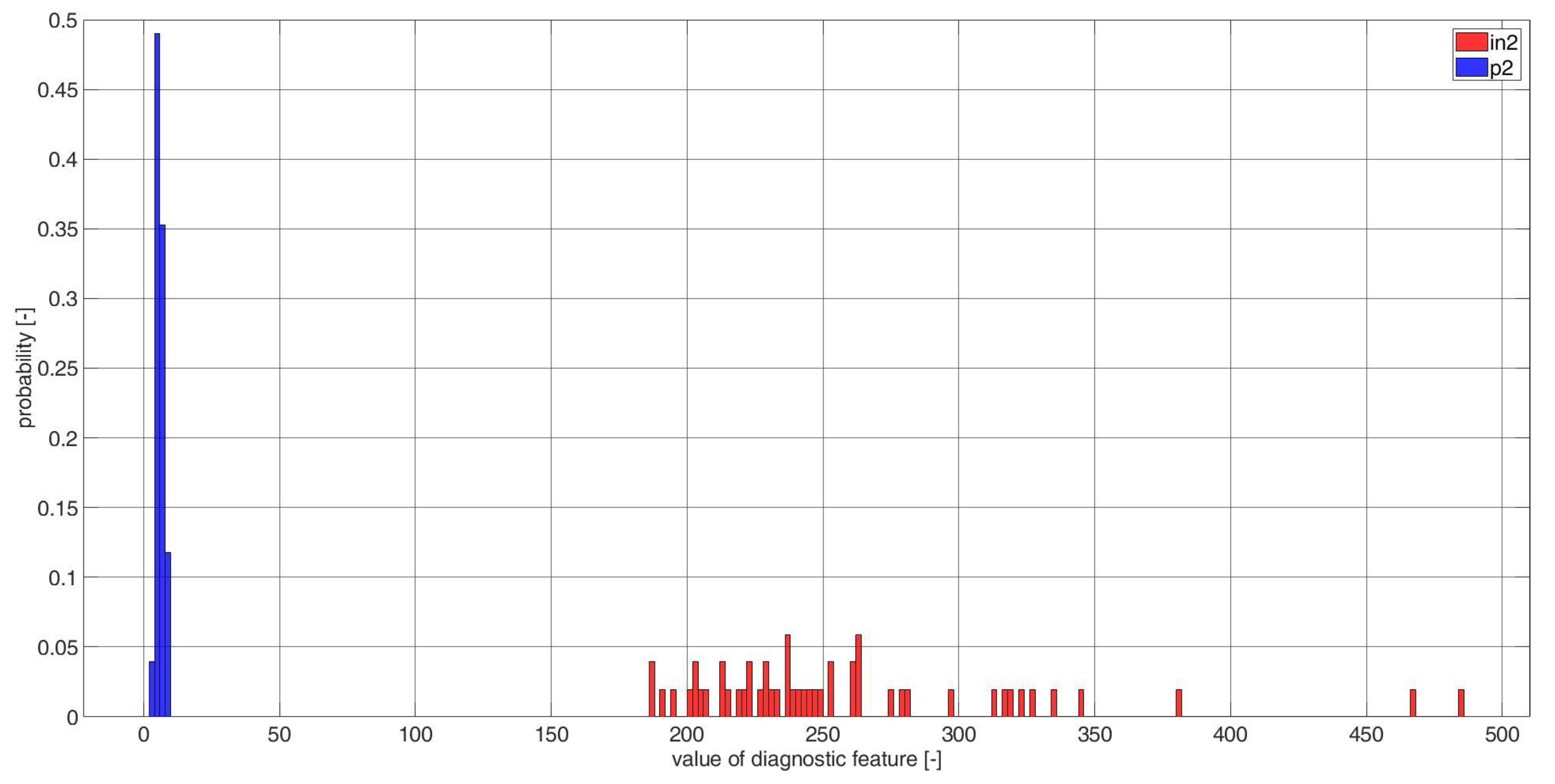
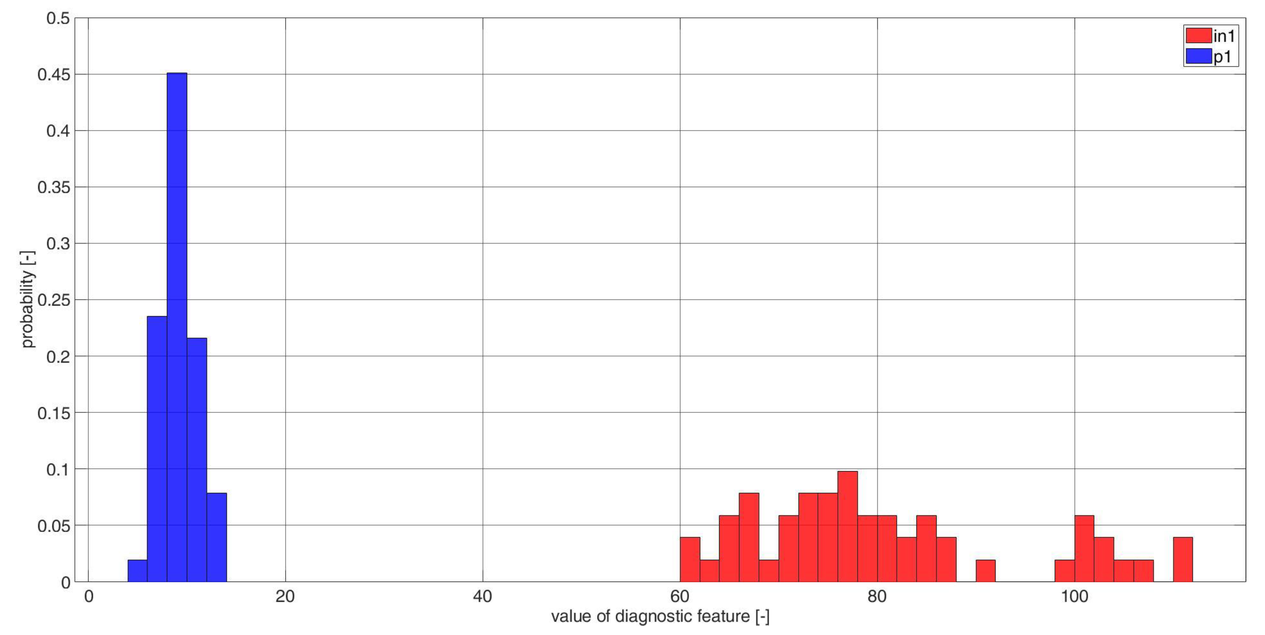
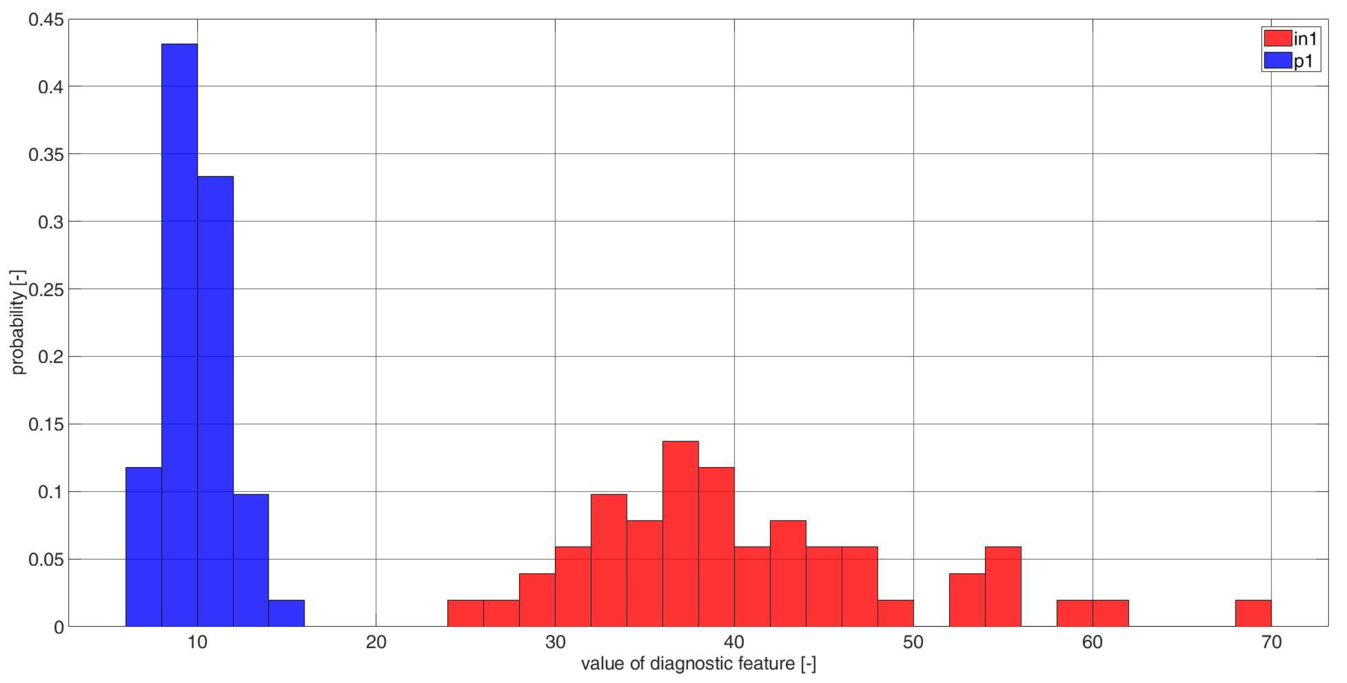
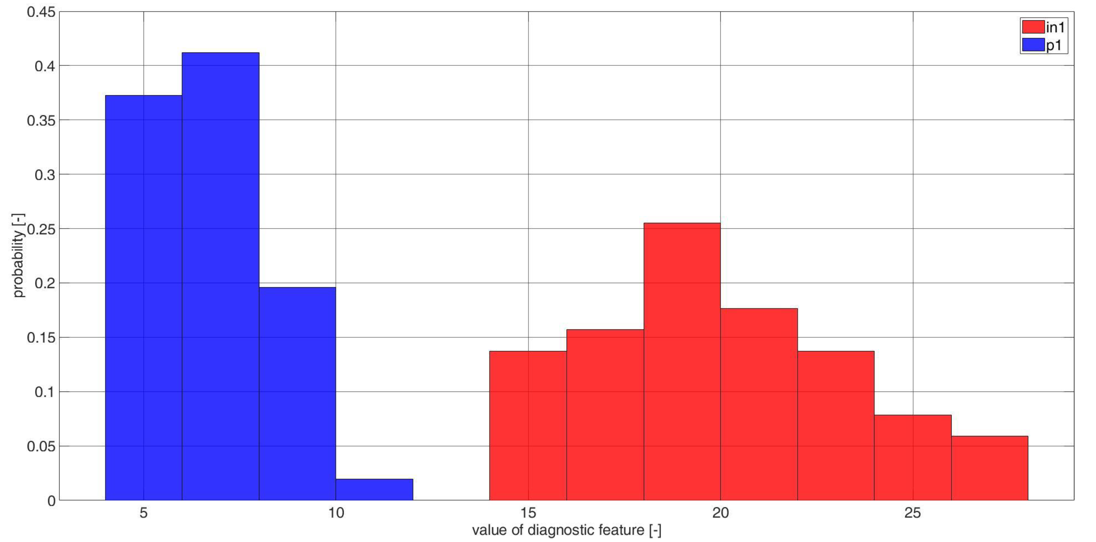
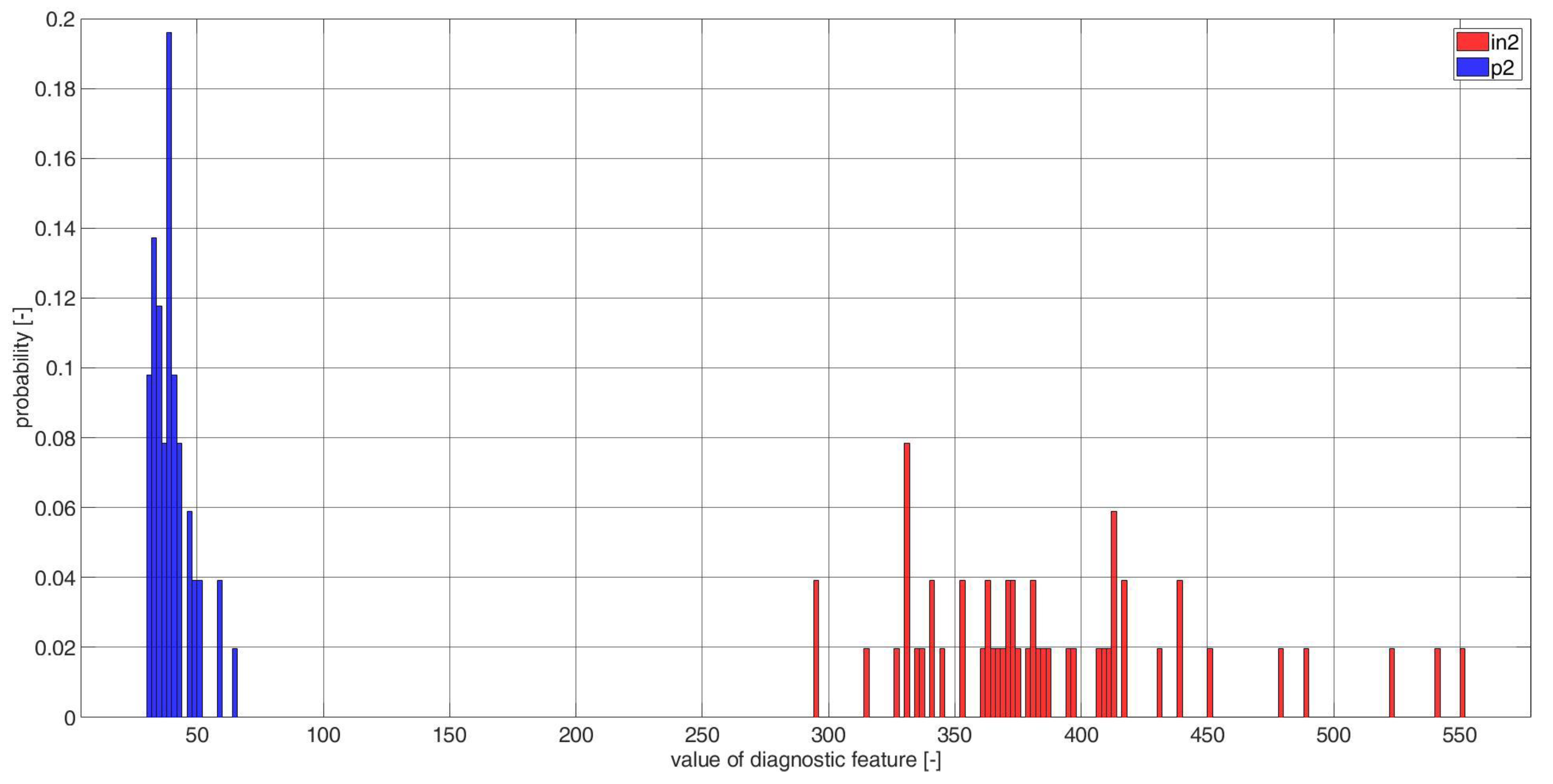
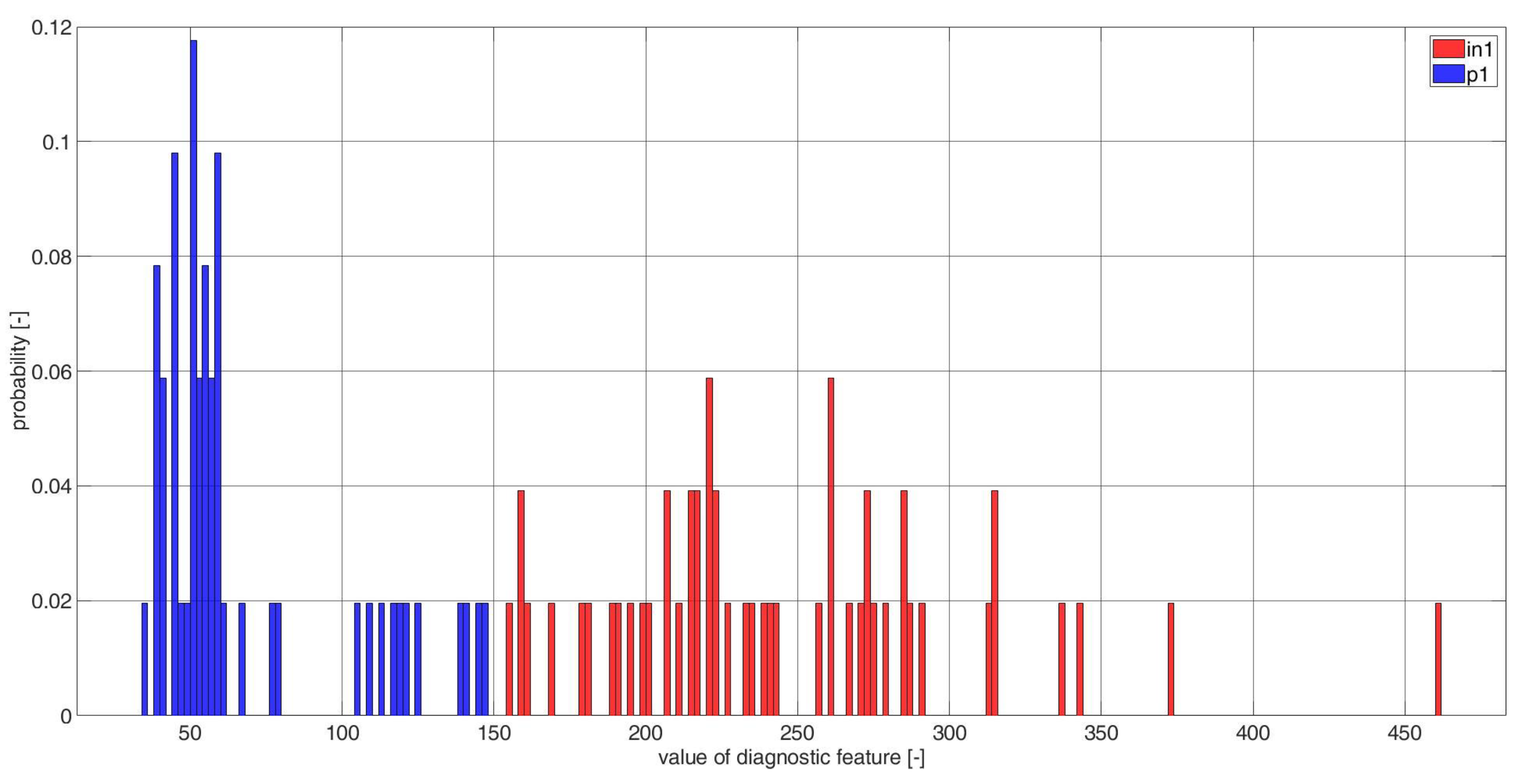
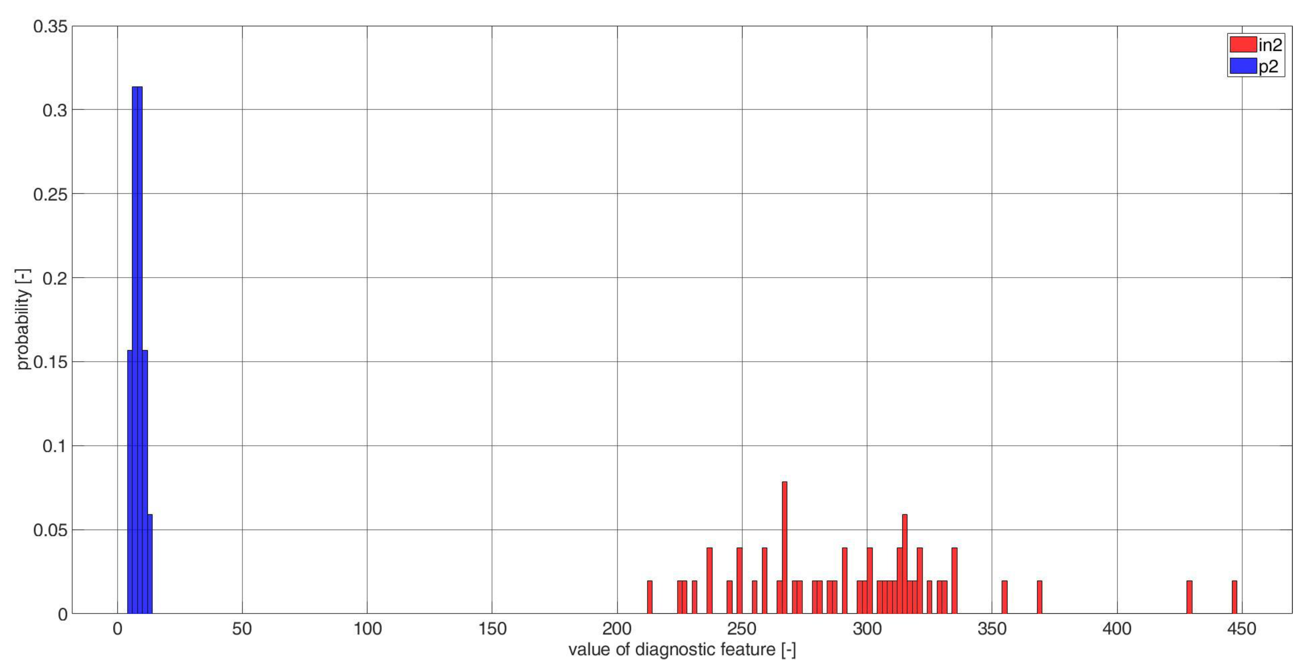
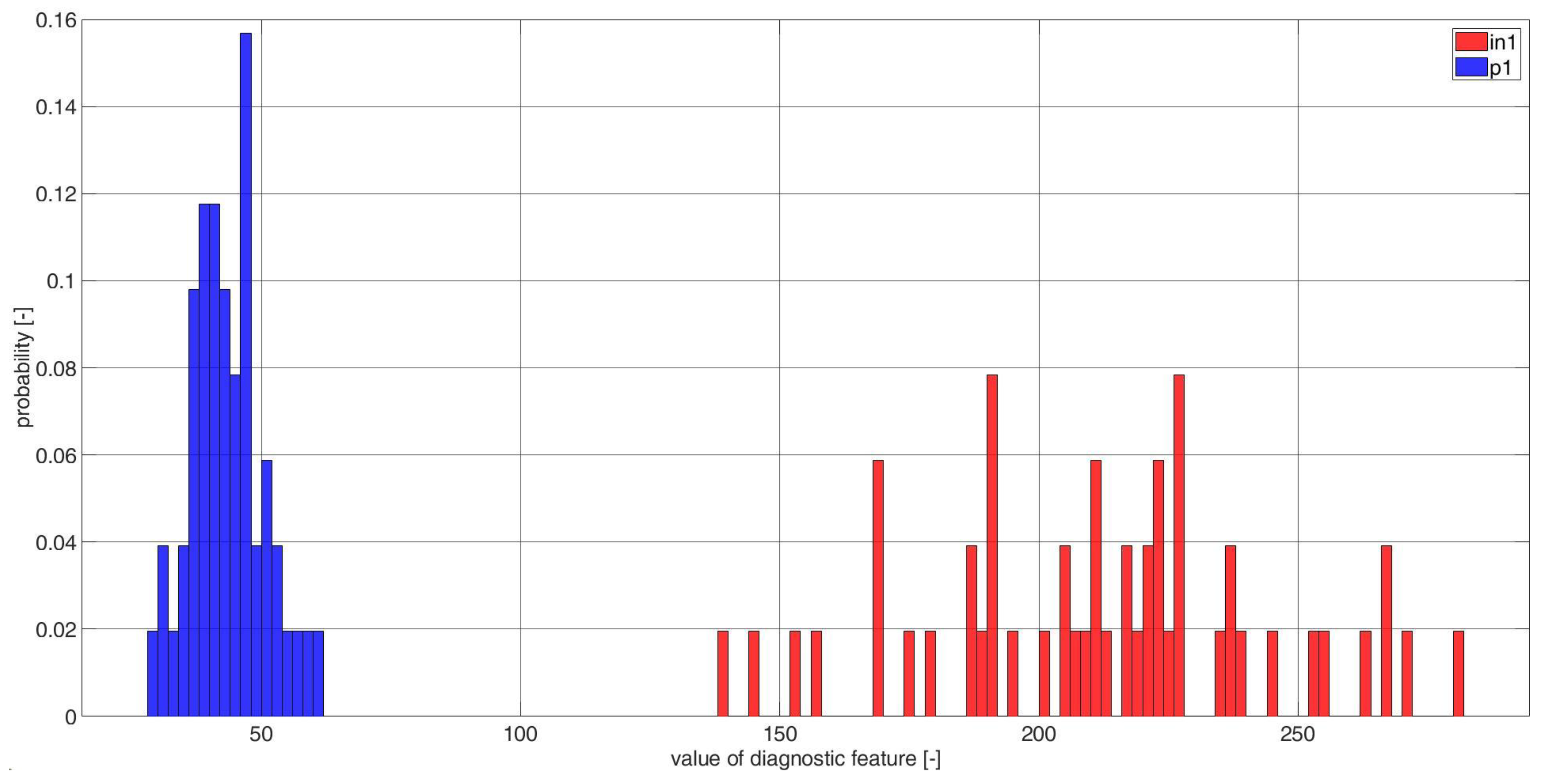
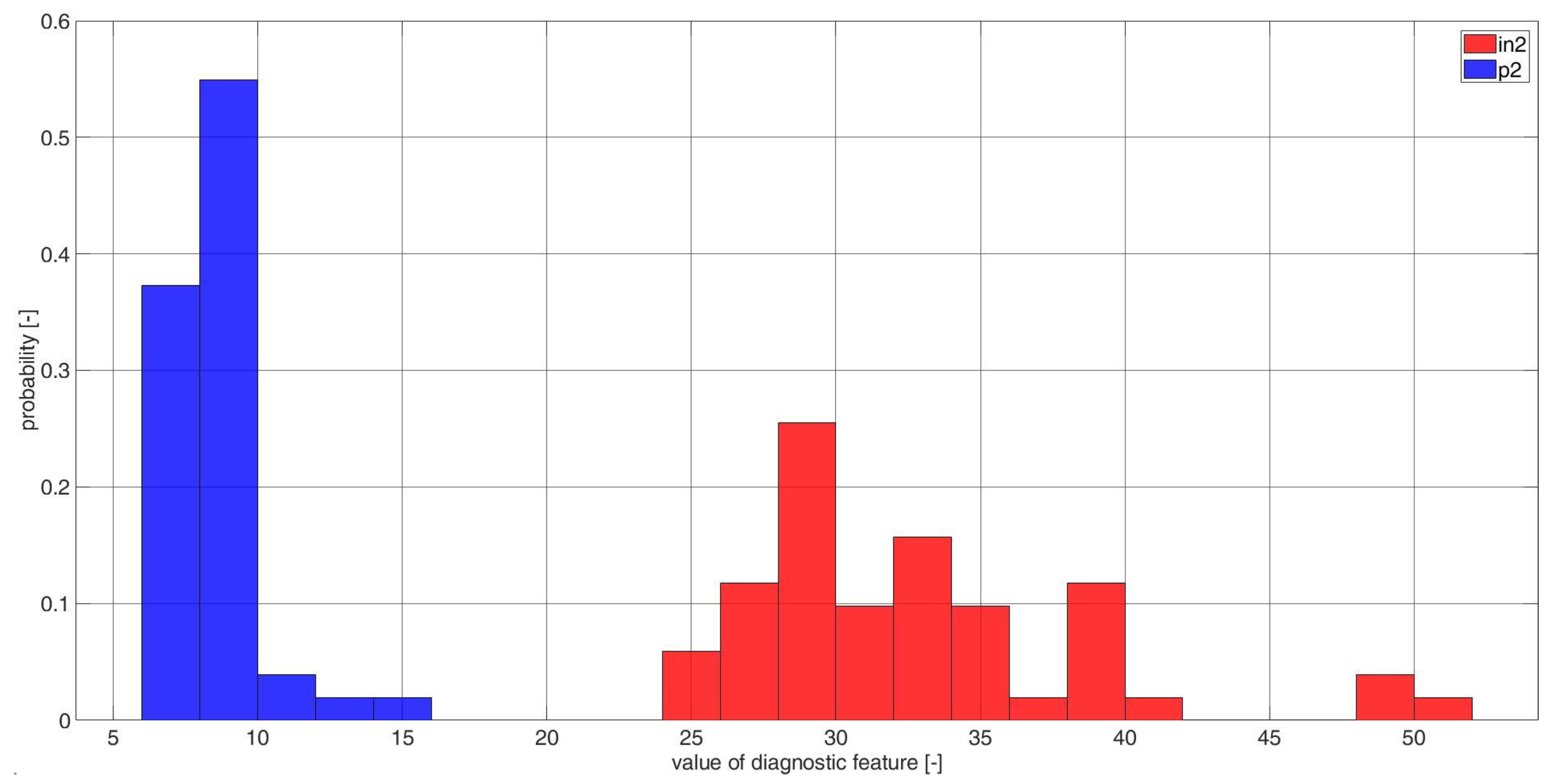
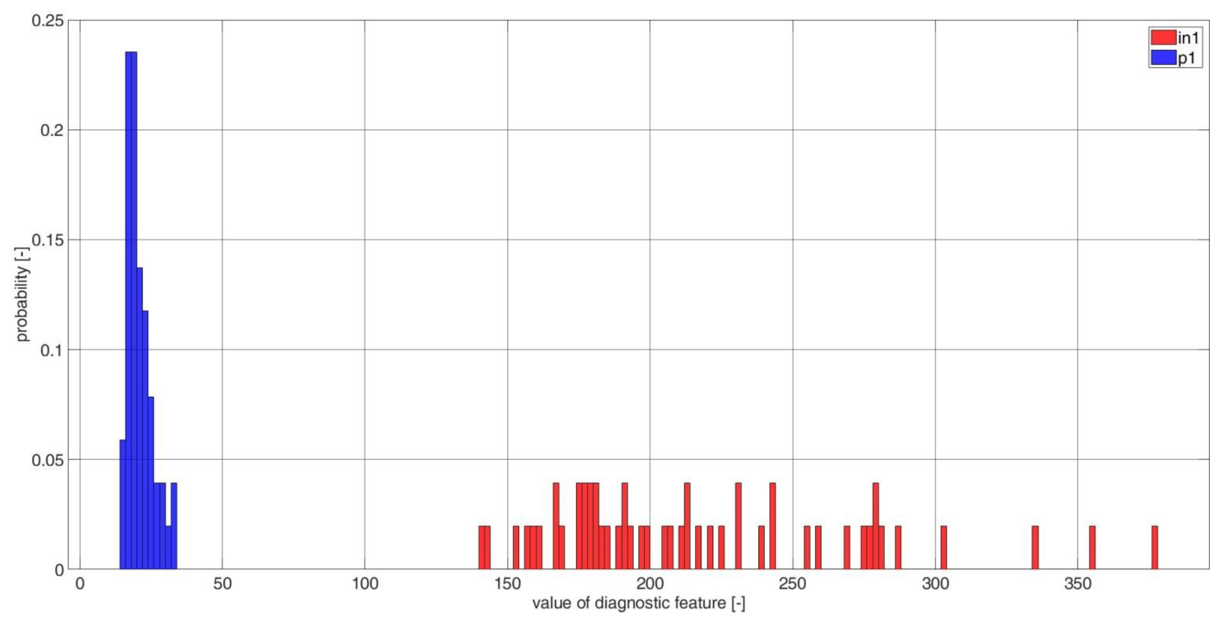
3.2. Local Inner Race Damage Diagnosis

Combination frequencies of current spectral components in raw current data, related to inner race bearing damage, are described by Equation (9) [9]:
f com _ in = i · f in + j · f g + k · f r
where f in is the inner race damage frequency (Equation (6)), f g is the fundamental frequency of supply current, f r is the fundamental motor shaft rotation frequency, and i , j , k are integer coefficients, related, respectively, to the inner race damage frequency, the fundamental frequency of supply current, and the fundamental motor rotation frequency.
The test bearings used for trials, were two damaged bearings: in1 and in2, and two pristine bearings, p1 and p2. The experimental results are based on 84 spectral components, which were used to calculate 28 CCSM3′s for each bearing. These 84 spectral components were obtained using the following coefficients:
i = 3, 6, 9;
j = −3, −1, 1, 3;
k = −3, −2, −1, 0, 1, 2, 3.
For each given i coefficient, a different set of j and k coefficients were used. This systematic set of 84 different components has been derived on the basis of the i , j , and   k coefficients. Each CCSM3 was calculated for multiple combinations of i , j , and   k values and averaged over three phases. Table A1 (Appendix A) presents multiple i , j ,   and   k combinations, corresponding to the correlation numbers for CCSM3. The overall probabilities of true diagnoses were estimated via Equation (7). The estimates of overall probabilities of true diagnoses, provided by CCSM3s, for each component combination, are shown in Figure 4. The estimate of the average overall probability of true diagnoses, calculated by averaging the estimates of overall probabilities, provided by all 28 CCSM3s, was 98.6%. The FCr, estimated for each component combination, are shown in Figure 5. The average FCr value provided by all 28 CCSM3s was 19.5.
Histograms of the diagnostic features, based on CCSM3 values for damaged and undamaged conditions, are presented in Figure 6 and Figure 7. The histograms of the selected CCSM3 diagnostic features are unimodal for both damaged and undamaged bearings. It can be seen from Figure 6 and Figure 7, that each pair of histograms show a full separation of diagnostic feature CCSMs between the damaged cases and the healthy cases. More histograms for other component combinations, based on CCSM3, for inner race fault diagnosis, are presented in Appendix A (Figure A1, Figure A2, Figure A3, Figure A4, Figure A5, Figure A6, Figure A7, Figure A8, Figure A9, Figure A10, Figure A11, Figure A12, Figure A13, Figure A14, Figure A15, Figure A16, Figure A17, Figure A18, Figure A19, Figure A20, Figure A21, Figure A22, Figure A23, Figure A24, Figure A25 and Figure A26). It can be seen from Figure A1, Figure A2, Figure A3, Figure A4, Figure A5, Figure A6, Figure A7, Figure A8, Figure A9, Figure A10, Figure A11, Figure A12, Figure A13, Figure A14, Figure A15, Figure A16, Figure A17, Figure A18, Figure A19, Figure A20, Figure A21, Figure A22, Figure A23, Figure A24, Figure A25 and Figure A26, that each pair of histograms, presented in the Appendix A, also show a full separation of diagnostic feature CCSMs between the damaged cases and the healthy cases. For each case in which diagnostic features for damaged and undamaged conditions are fully separated, the estimate of the overall probability of correct diagnosis is 100%.

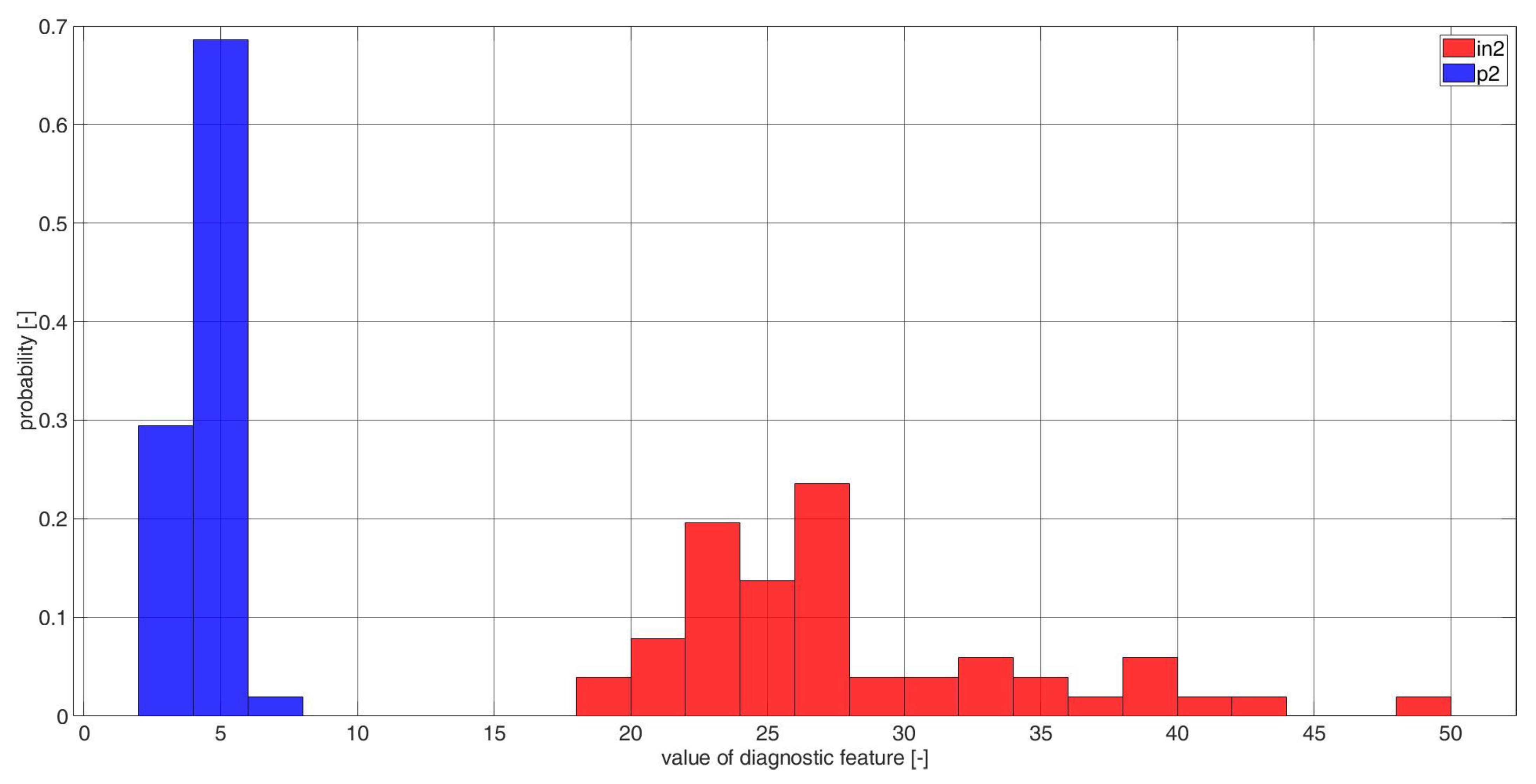
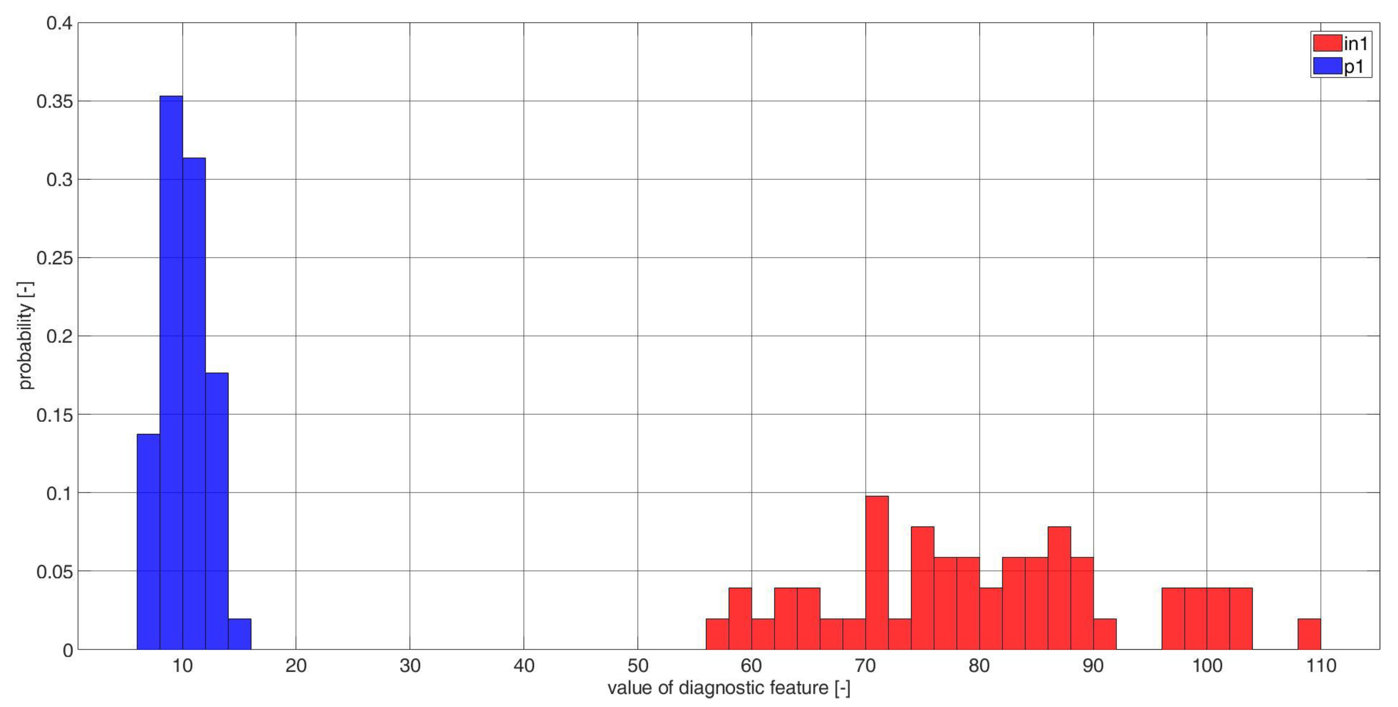
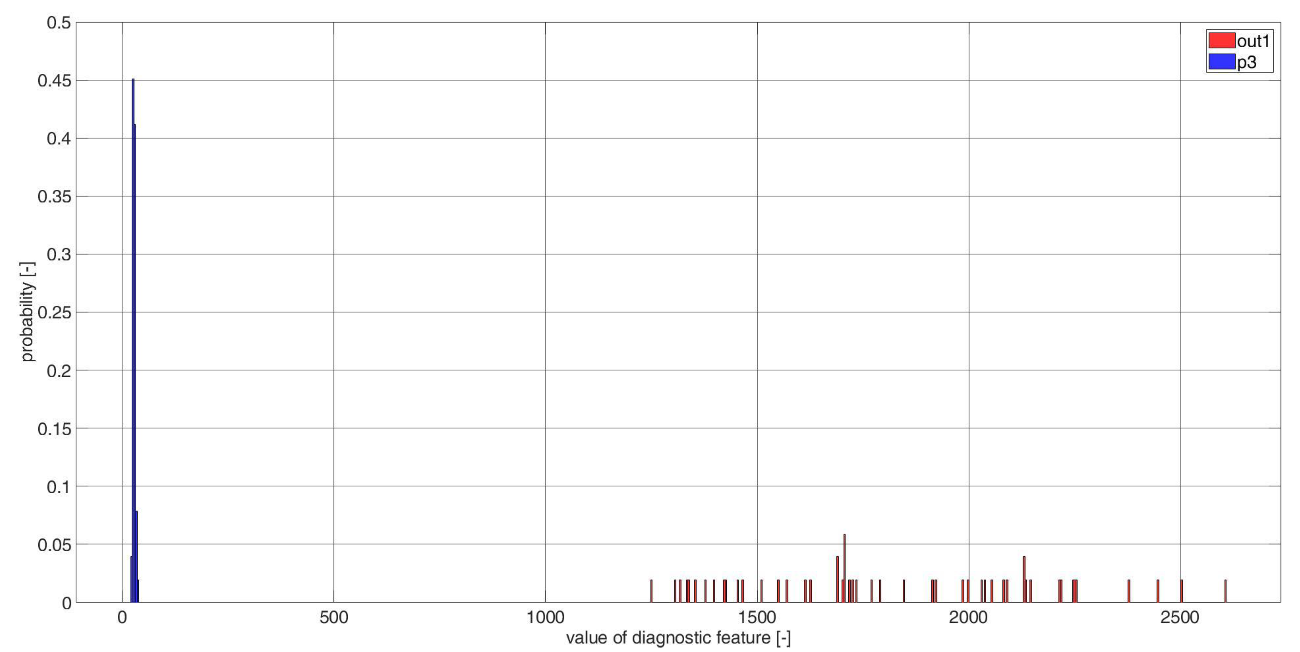
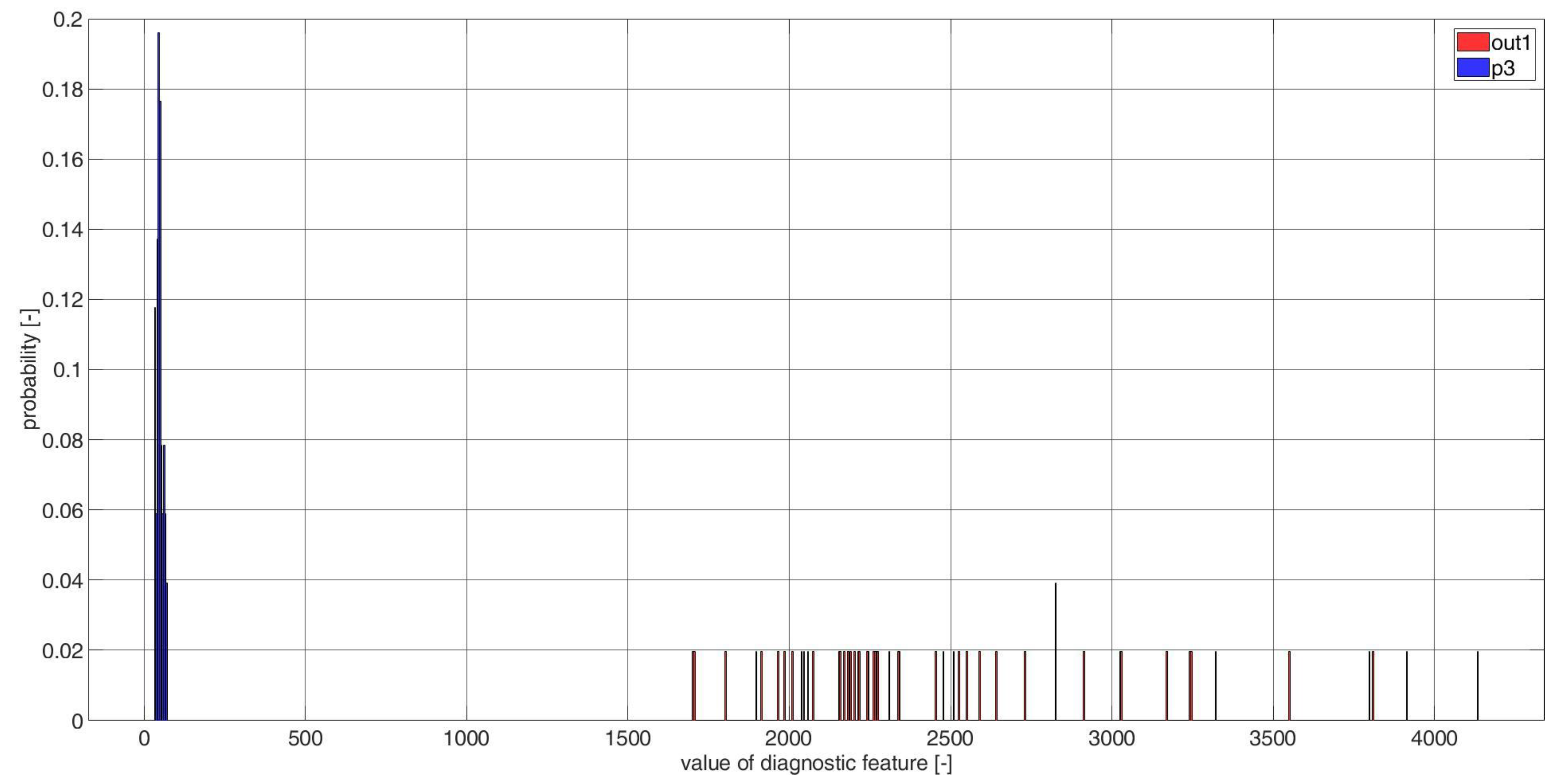
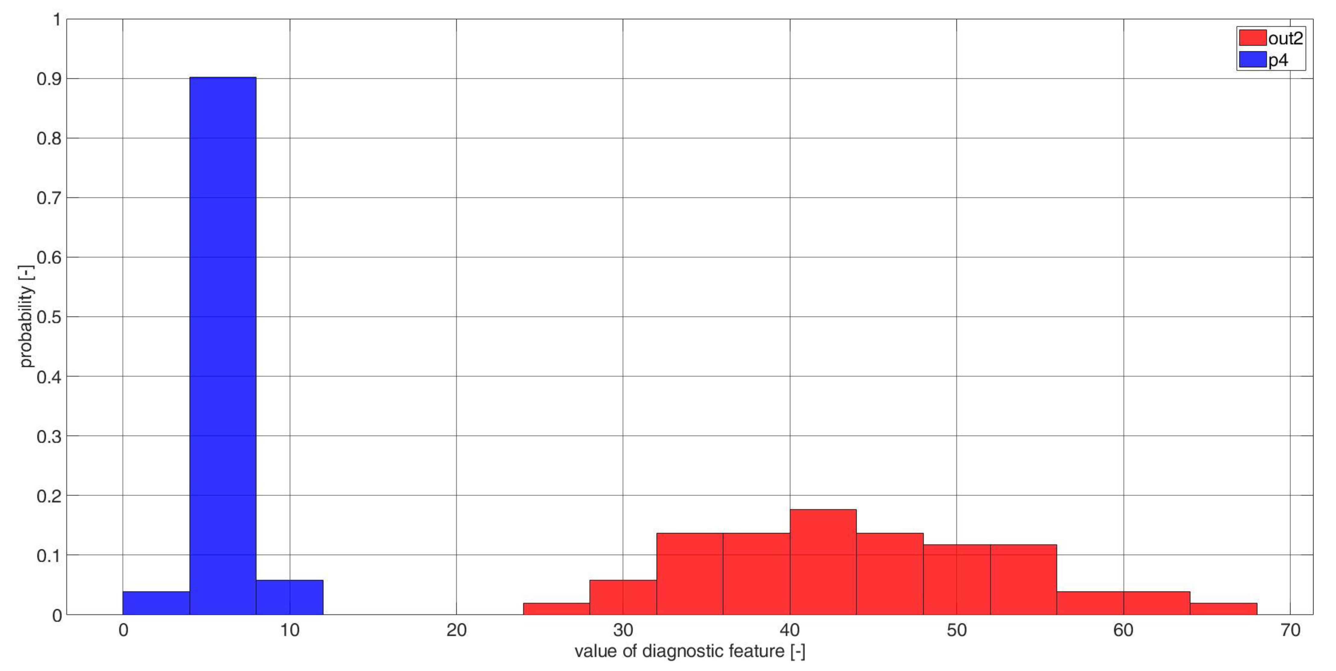
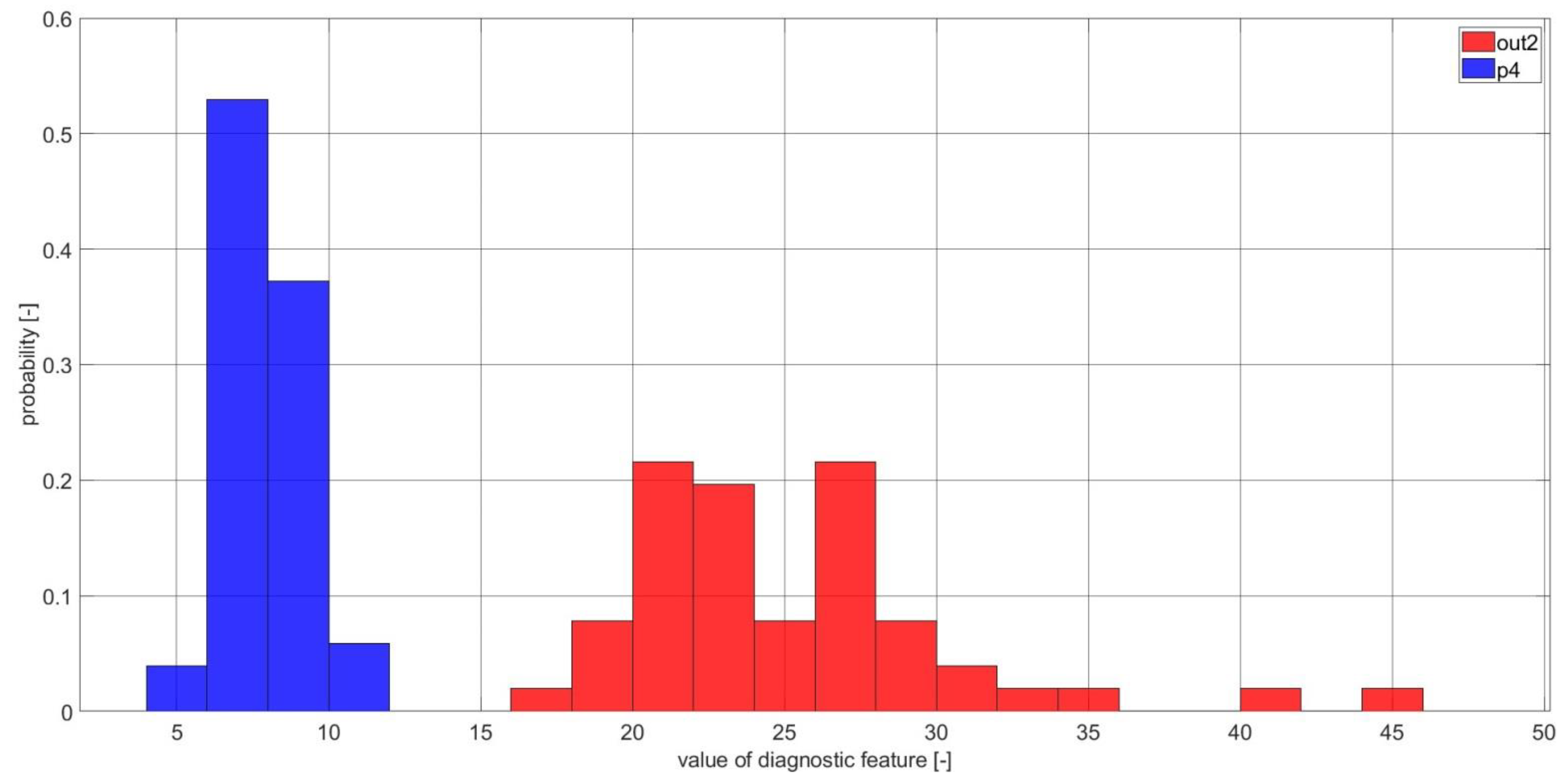
3.3. Outer Race Local Damage Diagnosis

Characteristic frequencies of current spectral components, related to the bearing outer race damage, in raw current data can be described by Equation (10) [8,9,10]:
f com _ out = i · f out + j · f g
where f out is the outer race damage frequency (Equation (5)), f g is the fundamental frequency of supply current, and i   and   j are integer coefficients, related, respectively, to the outer race damage frequency and the fundamental frequency of supply current.
Test bearings, that were used for trials, were damaged bearings out1, out2, and pristine bearings p3 and p4. The experimental trials are based on 12 components, which are used to calculate 4 CCSM3s for each bearing. The 12 components were obtained for the following coefficients:
i = 4, 8;
j = −5, −3, −1, 1, 3, 5.
For each given i coefficient, a different set of j coefficients were used. This systematic set of 12 different components were derived on the basis of the i and j coefficients. Each CCSM3 was calculated for an individual combination of i and j values, and averaged over three phases. Table A2 (Appendix A) presents multiple i and j combinations corresponding to the correlation number for CCSM3 estimation. The estimates of overall probabilities of correct diagnoses for the CCSM3 of each component combination, are shown in Figure 8. The estimate of the average overall probability of correct diagnoses, calculated by averaging the estimates of overall probabilities, evaluated for all 4 correlations, was 98.0%. FCr, calculated for each component combination, are shown in the Figure 9. Average value of FCr for all CCSM3 correlations, estimated by averaging FCr, provided by all 4 CCSM3s, was 13.2.
Histograms of the selected diagnostic features, based on CCSM3, are presented in Figure 10 and Figure 11. These histograms are unimodal for both the damaged and the undamaged bearings. It can be seen from Figure 10 and Figure 11, that each pair of histograms show a full separation of diagnostic feature CCSMs between the damaged and the undamaged cases. More histograms of other component combinations, based on the CCSM3 for outer race fault diagnosis, are presented in Appendix A (Figure A27, Figure A28, Figure A29, Figure A30 and Figure A31). It can be seen from Figure A27, Figure A28, Figure A29, Figure A30 and Figure A31, that each pair of histograms, presented in the Appendix A, also show a full separation of diagnostic feature CCSMs between the damaged cases and the healthy cases. For each case, in which diagnostic features for damaged and undamaged conditions, are fully separated, the estimate of the overall probability of correct diagnosis is 100%.
To conduct a novel comparison of bearing diagnosis results, provided by the proposed CCSM3 technology, and the state-of-the-art technology from [1], experimental current data from [1], captured from the damaged (i.e., outer race damage) bearing and the undamaged bearing were used. For the purpose of comparing the CCSM3 technology with the triple spectral cross-covariance technology [1], based on the complex Fourier transform, the same:
  • coefficients i   and   j (Equation (10)) for the three characteristic spectral components are used for CCSM3 technology as in [1]: i.e., 1,1; 2,1, and 1, −1
  • processing parameters: i.e., 65.536 kHz sampling frequency, 5 s time segment, signal duration is 65 s, overlap, varying from 0 to 50%, with a 1% step, are used for CCSM3 technology as in [1]
  • normalization of unnormalized correlations/covariances
  • number of diagnostic features for damaged and undamaged bearings are used for CCSM3 technology as in [1]
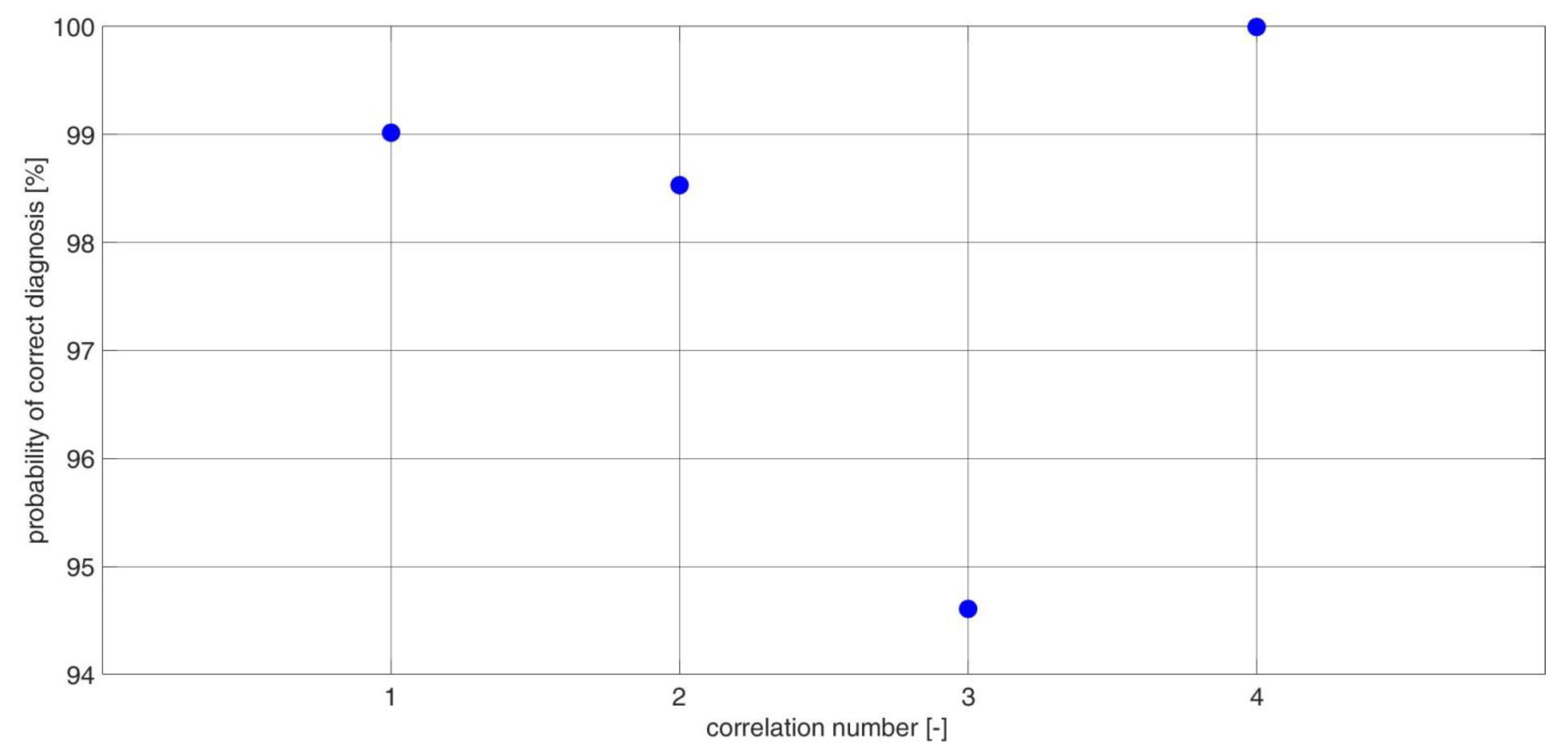
  • the Bayes decision-making method is used for CCSM3 technology as in [1].
For experimental bearing data from [1], the value of the FCr, achieved by CCSM3 technology, was 29.2 and a full separation of histograms for the CCSM3 diagnostic features for undamaged and damaged bearings was achieved; therefore, the estimate of the overall probability of error diagnostics, provided by CCSM3 technology, was 0%. Values of the FCr and the estimate of the overall probability of error diagnostics, achieved by the triple spectral cross-covariance technology presented in [1], were 6.7 and 4%, respectively. Gain in diagnosis effectiveness in terms of the FCr, calculated as a ratio of the FCr for the CCSM3 and the FCr for the triple spectral cross-covariance technology, was 4.4. This comparison also revealed, that the CCSM3 technology allows an essential decrease (i.e., 4%) in the overall probability of error diagnosis compared with the triple spectral cross-covariance technology.
The presented comparison results clearly show, that the proposed new CCSM3 technology, based on moduli of the Fourier transform (FT), is more efficient than the triple spectral cross-covariance technology, based on the complex FT.
The simulation results in [1] have shown that the triple spectral cross-covariance technology could effectively diagnose 5% relative damage size at signal to noise ratio (SNR) 30 dB. It has been shown above that the proposed technology outperforms the triple spectral cross-covariance technology. Therefore, the admissible SNR for the proposed technology is 30 dB for diagnosing 5% relative damage size.

4. Conclusions

1. For the first time worldwide, novel technologies for system diagnosis, the generic, non-linear higher-order, unnormalized cross-correlations of spectral moduli, related to steady and non-steady functioning of systems, has been proposed. Normally, normalization of higher-order correlations of random variables is based on the absolute central moments of order n, proposed and widely investigated in many mathematical works, e.g., [53,54,55,56,57].
The main difference between the proposed technologies and the higher-order, cross-covariance technologies in [1,2,3] and the classical higher-order spectra, is that the proposed cross-correlations are estimated for the spectral moduli of the selected characteristic spectral components. The proposed use of moduli of complex transforms for higher-order spectral techniques is non-traditional, as traditionally, in all known applications of higher-order spectral techniques, the complex spectral components (not moduli of complex spectral components) are used.
The main novel contributions are the theoretical development and investigation of the proposed technologies. Further innovative contribution is the proposed capability of fault diagnosis for non-steady functioning of complex assets via the employment of non-stationary transforms for the proposed technologies.
2. The proposed technology, the cross-correlation of spectral moduli of order 3 (CCSM3), is employed for the performance of experimental trials in bearing damage diagnosis by MCSA. Experimental technology validations were carried out on 8 bearings: two bearings with inner race early damage, two bearings with outer race early damage, and four pristine bearings. In the “inner race damage” experiments, 28 different diagnosis features, averaged over three phases, were examined. In the “outer race damage” experiments, 4 different diagnosis features, averaged over three phases, were examined.
Experimental trials were undertaken via the test rig, dedicated for IM testing. Motor current signals were captured for 4 pristine and 4 damaged bearings. Experimental testing of the proposed diagnostic technique via MCSA, has shown, that the technology very effectively diagnosed bearing outer race and inner race faults at early stages of fault development, i.e., average overall probabilities of correct diagnostics of outer race and inner race damages were 98.0% and 98.6%, respectively.
3. For outer race experiments, local damage diagnostics were compared with local damage diagnostics, achieved in [1], using the same experimental data capture from damaged and undamaged bearings. Experimental comparison showed, that the CCSM3 was a more efficient signal processing technique than the triple spectral cross-covariance technology proposed in ref [1]. Experimental gain in the Fisher criterion for the CCSM3, in comparison with the technique in [1] is 4.4. It has been shown that the proposed CCSM3 technology allows essential decrease in the overall probability of error diagnosis, compared with the triple spectral cross-covariance technology. These experimental comparison results have shown that the proposed technology is superior to the current technology, based on complex spectral components [1] for bearing fault diagnosis via MCSA and therefore, it is an essential way forward for early damage diagnosis.
4. This study is foremost for damage diagnosis. The proposed cross-correlations of spectral moduli, present a novel conceptualization and will make a considerable impact on damage diagnosis for electrical and mechanical engineering, via motor current signature analysis, vibration analysis, ultrasound analysis, etc.

Author Contributions

Conceptualization, L.G. methodology, L.G., T.C. and A.B. software, T.C. validation, L.G. and T.C., investigation, L.G., T.C. and A.B., resources, T.C. data curation, T.C., writing—original draft preparation, T.C., writing—review and editing, L.G. and A.B. visualization, T.C., supervision, L.G. All authors have read and agreed to the published version of the manuscript.

Funding

This research received no external funding.

Acknowledgments

The authors would like to acknowledge and thank the following people: L. Swędrowski, M. Wołoszyk and M. Ziółko from Department of Metrology and Information Systems, Faculty of Electrical and Control Engineering of Gdansk University of Technology for design and completion of the test rig and to Phil Spry, SKF UK, for supplying bearing parameters.

Conflicts of Interest

The authors declare no conflict of interest.

Appendix A

Table A1. List of spectral components used for inner race diagnosis.
Correlation Number ijk
13−3−3
6−3−3
9−3−3
23−1−3
6−1−3
9−1−3
331−3
61−3
91−3
433−3
63−3
93−3
53−3−2
6−3−2
9−3−2
63−1−2
6−1−2
9−1−2
731−2
61−2
91−2
833−2
63−2
93−2
93−3−1
6−3−1
9−3−1
103−1−1
6−1−1
9−1−1
1131−1
61−1
91−1
1233−1
63−1
93−1
133−30
6−30
9−30
143−10
6−10
9−10
15310
610
910
16330
630
930
173−31
6−31
9−31
183−11
6−11
9−11
19311
611
911
20331
631
931
213−32
6−32
9−32
223−12
6−12
9−12
23312
612
912
24332
632
932
253−33
6−33
9−33
263−13
6−13
9−13
27313
613
913
28333
633
933
Figure A1. Histograms of diagnostic features based on the CCSM3 (correlation number is 4—Table A1) bearings in1 and p1.
Electronics 11 03885 g0a1
Figure A2. Histograms of diagnostic features based on the CCSM3 (correlation number is 4—Table A1) bearings in2 and p2.
Electronics 11 03885 g0a2
Figure A3. Histograms of diagnostic features based on the CCSM3 (correlation number is 5—Table A1) bearings in1 and p1.
Electronics 11 03885 g0a3
Figure A4. Histograms of diagnostic features based on the CCSM3 (correlation number is 5—Table A1) bearings in2 and p2.
Electronics 11 03885 g0a4
Figure A5. Histograms of diagnostic features based on the CCSM3 (correlation number is 6—Table A1) bearings in1 and p1.
Electronics 11 03885 g0a5
Figure A6. Histogram of diagnostic features based on the CCSM3 (correlation number is 6—Table A1) bearings in2 and p2.
Electronics 11 03885 g0a6
Figure A7. Histograms of diagnostic features based on the CCSM3 (correlation number is 7—Table A1) bearings in1 and p1.
Electronics 11 03885 g0a7
Figure A8. Histograms of diagnostic features based on the CCSM3 (correlation number is 7—Table A1) bearings in2 and p2.
Electronics 11 03885 g0a8
Figure A9. Histograms of diagnostic features based on the CCSM3 (correlation number is 8—Table A1) bearings in1 and p1.
Electronics 11 03885 g0a9
Figure A10. Histograms of diagnostic features based on the CCSM3 (correlation number is 8—Table A1) bearings in2 and p2.
Electronics 11 03885 g0a10
Figure A11. Histograms of diagnostic features based on the CCSM3 (correlation number is 10—Table A1) bearings in1 and p1.
Electronics 11 03885 g0a11
Figure A12. Histograms of diagnostic features based on the CCSM3 (correlation number is 12—Table A1) bearings in2 and p2.
Electronics 11 03885 g0a12
Figure A13. Histograms of diagnostic features based on the CCSM3 (correlation number is 12—Table A1) bearings in1 and p1.
Electronics 11 03885 g0a13
Figure A14. Histograms of diagnostic features based on the CCSM3 (correlation number is 12—Table A1) bearings in2 and p2.
Electronics 11 03885 g0a14
Figure A15. Histograms of diagnostic features based on the CCSM3 (correlation number is 13—Table A1), bearings in1 and p1.
Electronics 11 03885 g0a15
Figure A16. Histograms of diagnostic features based on the CCSM3 (correlation number is 13—Table A1) bearings in2 and p2.
Electronics 11 03885 g0a16
Figure A17. Histograms of diagnostic features based on the CCSM3 (correlation number is 20—Table A1) bearings in1 and p1.
Electronics 11 03885 g0a17
Figure A18. Histograms of diagnostic features based on the CCSM3 (correlation number is 20—Table A1) bearings in2 and p2.
Electronics 11 03885 g0a18
Figure A19. Histograms of diagnostic features based on the CCSM3 (correlation number is 21—Table A1) bearings in1 and p1.
Electronics 11 03885 g0a19
Figure A20. Histograms of diagnostic features based on the CCSM3 (correlation number is 21—Table A1) bearings in2 and p2.
Electronics 11 03885 g0a20
Figure A21. Histograms of diagnostic features based on the CCSM3 (correlation number is 22—Table A1) bearings in1 and p1.
Electronics 11 03885 g0a21
Figure A22. Histograms of diagnostic features based on the CCSM3 (correlation number is 22—Table A1) bearings in2 and p2.
Electronics 11 03885 g0a22
Figure A23. Histograms of diagnostic features based on the CCSM3 (correlation number is 24—Table A1) bearings in1 and p1.
Electronics 11 03885 g0a23
Figure A24. Histograms of diagnostic features based on the CCSM3 (correlation number is 24—Table A1) bearings in2 and p2.
Electronics 11 03885 g0a24
Figure A25. Histograms of diagnostic features based on the CCSM3 (correlation number is 28—Table A1) bearings in1 and p1.
Electronics 11 03885 g0a25
Figure A26. Histograms of diagnostic features based on the CCSM3 (correlation number is 28—Table A1) bearings in2 and p2.
Electronics 11 03885 g0a26
Table A2. List of spectral components, used for outer race diagnosis.
Correlation Number ij
14−5
4−3
4−1
241
43
45
38−5
8−3
8−1
481
83
85
Figure A27. Histogram of diagnostic features based on the CCSM3 (correlation number is 1—Table A2) bearings out1 and p3.
Electronics 11 03885 g0a27
Figure A28. Histograms of diagnostic features based on the CCSM3 (correlation number is 1—Table A2) bearings out2 and p4.
Electronics 11 03885 g0a28
Figure A29. Histograms of diagnostic features based on the CCSM3 (correlation number is 2—Table A2) bearings out1 and p3.
Electronics 11 03885 g0a29
Figure A30. Histograms of diagnostic features based on the CCSM3 (correlation number is 3—Table A2) bearings out1 and p3.
Electronics 11 03885 g0a30
Figure A31. Histograms of diagnostic features based on the CCSM3 (correlation number is 3—Table A2) bearings out2 and p4.
Electronics 11 03885 g0a31

References

  1. Ciszewski, T.; Gelman, L.; Ball, A. Novel fault identification for electromechanical systems via spectral technique and electrical data processing. Electronics 2020, 9, 1560. [Google Scholar] [CrossRef]
  2. Gelman, L.; Soliński, K.; Ball, A. Novel higher-order spectral cross-correlation technologies for vibration sensor-based diagnosis of gearboxes. Sensors 2020, 20, 5131. [Google Scholar] [CrossRef]
  3. Ciszewski, T.; Gelman, L.; Swędrowski, L. Current-based higher-order spectral covariance as a bearing diagnostic feature for induction motors. Insight-Non-Destr. Test. Cond. Monit. 2016, 58, 431–434. [Google Scholar] [CrossRef]
  4. Schoen, R.; Habetler, T.G.; Kamran, F.; Bartheld, R.G. Motor bearing damage detection, using stator current monitoring. IEEE Trans. Ind. Appl. 1995, 31, 6. [Google Scholar] [CrossRef]
  5. Areias, I.A.d.S.; Borges da Silva, L.E.; Bonaldi, E.L.; de Lacerda de Oliveira, L.E.; Lambert-Torres, G.; Bernardes, V.A. Evaluation of Current Signature in Bearing Defects by Envelope Analysis of the Vibration in Induction Motors. Energies 2019, 12, 4029. [Google Scholar] [CrossRef] [Green Version]
  6. Singh, S.; Kumar, N. Detection of Bearing Faults in Mechanical Systems Using Stator Current Monitoring. IEEE Trans. Ind. Inform. 2017, 13, 1341–1349. [Google Scholar] [CrossRef]
  7. Gangsar, P.; Tiwari, R. Signal based condition monitoring techniques for fault detection and diagnosis of induction motors: A state-of-the-art review. Mech. Syst. Signal Process. 2020, 144, 106908. [Google Scholar] [CrossRef]
  8. Han, Q.; Ding, Z.; Xu, X.; Wang, T.; Chu, F. Stator current model for detecting rolling bearing faults in induction motors using magnetic equivalent circuits. Mech. Syst. Signal Process. 2019, 131, 554–575. [Google Scholar] [CrossRef]
  9. Blödt, M.; Granjon, P.; Raison, B.; Rostaing, G. Models for Bearing Damage Detection in Induction Motors Using Stator Current Monitoring. IEEE Trans. Ind. Electron. 2008, 55, 1813–1822. [Google Scholar] [CrossRef] [Green Version]
  10. Acosta, G.G.; Verucchi, C.J.; Gelso, E.R. A current monitoring system for diagnosing electrical failures in induction motors. Mech. Syst. Signal Proc. 2006, 20, 953–965. [Google Scholar] [CrossRef]
  11. Gelman, L.; Chandra, N.H.; Kurosz, R.; Pellicano, F.; Barbieri, M.; Zippo, A. Novel spectral kurtosis technology for adaptive vibration condition monitoring of multi-stage gearboxes. Insight-Non-Destr. Test. Cond. Monit. 2016, 58, 409–416. [Google Scholar] [CrossRef]
  12. Combet, F.; Gelman, L.; Anuzis, P.; Slater, R. Vibration detection of local gear damage by advanced demodulation and residual techniques, Proceedings of the Institution of Mechanical Engineers. Part G J. Aerosp. Eng. 2009, 223, 507–514. [Google Scholar] [CrossRef]
  13. Gryllias, K.; Gelman, L.; Shaw, B.; Vaidhianathasamy, M. Local damage diagnosis in gearboxes using novel wavelet technology. Int. J. Insight-Non-Destr. Test. Cond. Monit. 2010, 52, 437–442. [Google Scholar] [CrossRef]
  14. Gelman, L.; Kripak, D.A.; Fedorov, V.V.; Udovenko, L.N. Condition monitoring diagnosis methods of helicopter units. Mech. Syst. Signal Process. 2000, 14, 613–624. [Google Scholar] [CrossRef]
  15. Kolbe, S.; Gelman, L.; Ball, A. Novel prediction of diagnosis effectiveness for adaptation of the spectral kurtosis technology to varying operating conditions. Sensors 2021, 21, 6913. [Google Scholar] [CrossRef] [PubMed]
  16. Gelman, L.; Soliński, K.; Ball, A. Novel instantaneous wavelet bicoherence for vibration fault detection in gear systems. Energies 2021, 14, 6811. [Google Scholar] [CrossRef]
  17. Gelman, L.; Kolbe, S.; Shaw, B.; Vaidhianathasamy, M. Novel adaptation of the spectral kurtosis for vibration diagnosis of gearboxes in non-stationary conditions. Int. J. Insight-Non-Destr. Test. Cond. Monit. 2017, 59, 434–439. [Google Scholar] [CrossRef]
  18. Gelman, L.; Solinski, K.; Shaw, B.; Vaidhianathasamy, M. Vibration diagnosis of a gearbox by wavelet bicoherence technology. Int. J. Insight-Non-Destr. Test. Cond. Monit. 2017, 59, 440–444. [Google Scholar] [CrossRef] [Green Version]
  19. Corne, B.; Vervisch, B.; Derammelaere, S.; Knockaert, J.; Desmet, J. The reflection of evolving bearing faults in the stator current’s extended park vector approach for induction machines. Mech. Syst. Signal Process. 2018, 107, 168–182. [Google Scholar] [CrossRef]
  20. Silva, J.L.H.; Cardoso, A.J.M. Bearing failures diagnosis in three-phase induction motors by extended Park’s vector approach. In Proceedings of the 31st Annual Conference of IEEE Industrial Electronics Society, 2005. IECON 2005, Raleigh, NC, USA, 6–10 November 2005. [Google Scholar]
  21. Wang, C.; Wang, M.; Yang, B.; Song, K.; Zhang, Y.; Liu, L. A novel methodology for fault size estimation of ball bearings using stator current signal. Measurement 2021, 171, 108723. [Google Scholar] [CrossRef]
  22. Treetrong, J. Fault Detection and Diagnosis of Induction Motors Based on Higher-Order Spectrum. In Proceedings of the International Multi Conference of Engineers and Computer Scientists, Honk Kong, China, 17–19 May 2010; Volume II. [Google Scholar]
  23. Song, X.; Hu, J.; Zhu, H.; Zhang, J. A Bearing Outer Raceway Fault Detection Method in Induction Motors Based on Instantaneous Frequency of the Stator Current. IEEJ Trans. Electr. Electron. Eng. 2018, 13, 510–516. [Google Scholar] [CrossRef]
  24. Tulicki, J.; Sułowicz, M.; Pragłowska-Ryłko, N. Application of the Bispectral Analysis in the Diagnosis of Cage Induction Motors. In Proceedings of the 2016 13th Selected Issues of Electrical Engineering and Electronics (WZEE), Rzeszow, Poland, 4–8 May 2016. [Google Scholar] [CrossRef]
  25. Zhao, D.; Gelman, L.; Chu, F.; Ball, A. Vibration health monitoring of rolling bearings under variable speed conditions by novel demodulation technique. Struct. Control. Health Monit. 2020, 28, e2672. [Google Scholar] [CrossRef]
  26. Gelman, L.; Patel, T.H.; Persin, G.; Murray, B.; Thomson, A. Novel technology based on the spectral kurtosis and wavelet transform for rolling bearing diagnosis. Int. J. Progn. Health Manag. 2013, 4, 2153–2648. [Google Scholar] [CrossRef]
  27. Gelman, L.; Murray, B.; Patel, T.H.; Thomson, A. Vibration diagnostics of rolling bearings by novel nonlinear non-stationary wavelet bicoherence technology. Eng. Struct. 2014, 80, 514–520. [Google Scholar] [CrossRef]
  28. Gelman, L.; Persin, G. Novel fault diagnosis of bearings and gearboxes based on simultaneous processing of spectral kurtoses. Appl. Sci. 2022, 12, 9970. [Google Scholar] [CrossRef]
  29. Zarei, J.; Poshtan, J. An Advanced Park’s Vectors Approach for Bearing Fault Detection. IEEE Int. Conf. Ind. Technol. 2006, 42, 213–219. [Google Scholar] [CrossRef]
  30. Gao, Z.; Turner, L.; Colby, R.S.; Leprettre, B. Frequency Demodulation Approach to Induction Motor Speed Detection. IEEE Trans. Ind. Appl. 2011, 47, 730–738. [Google Scholar] [CrossRef]
  31. Eren, L.; Karahoca, A.; Devaney, M.J. Neural network based motor bearing fault detection. In Proceedings of the 21st IEEE Instrumentation and Measurement Technology Conference, Como, Italy, 18–20 May 2004; Volume 3, pp. 1657–1660. [Google Scholar] [CrossRef]
  32. Eren, L.; Teotrakool, K.; Devaney, M.J. Bearing fault detection via wavelet packet decomposition with spectral post processing. In Proceedings of the 2007 IEEE Instrumentation & Measurement Technology Conference IMTC 2007, Warsaw, Poland, 1–3 May 2007; pp. 1–4. [Google Scholar] [CrossRef]
  33. Nikolaou, N.G.; Antoniadis, I.A. Rolling element bearing fault diagnosis using wavelet packets. NDT E Int. 2002, 35, 197–205. [Google Scholar] [CrossRef]
  34. Lou, X.; Loparo, K. Bearing fault diagnosis based on wavelet transform and fuzzy inference. Mech. Syst. Signal Process. 2004, 18, 1077–1095. [Google Scholar] [CrossRef]
  35. Yaqub, M.F.; Loparo, K.A. An automated approach for bearing damage detection. J. Vib. Control. 2016, 22, 3253–3266. [Google Scholar] [CrossRef]
  36. Yiakopoulos, C.; Antoniadis, I. Wavelet Based Demodulation of Vibration Signals Generated by Defects in Rolling Element Bearings. In Proceedings of the ASME 2001 International Design Engineering Technical Conferences and Computers and Information in Engineering Conference, Volume 6C: 18th Biennial Conference on Mechanical Vibration and Noise. Pittsburgh, PA, USA, 9–12 September 2001; pp. 3187–3195. [Google Scholar] [CrossRef]
  37. Dahiya, N.M.R. Detection of Bearing Faults of Induction Motor Using Park’s Vector Approach. Int. J. Eng. 2010, 1, 263–266. [Google Scholar]
  38. Saeidi, M.; Zarei, J.; Hassani, H.; Zamani, A.; Majid, S. Bearing fault detection via Park’s vector approach based on ANFIS. In Proceedings of the 2014 International Conference on Mechatronics and Control (ICMC), Jinzhou, China, 3–5 July 2014. [Google Scholar] [CrossRef]
  39. Irfan, M.; Saad, N.; Ibrahim, R.; Asirvadam, V.S.; Alwadie, A. Analysis of distributed faults in inner and outer race of bearing via Park vector analysis method. Neural Comput. Appl. 2019, 31, 683–691. [Google Scholar] [CrossRef]
  40. Koteleva, N.; Korolev, N.; Zhukovskiy, Y.; Baranov, G. A Soft Sensor for Measuring the Wear of an Induction Motor Bearing by the Park’s Vector Components of Current and Voltage. Sensors 2021, 21, 7900. [Google Scholar] [CrossRef] [PubMed]
  41. Zarei, J.; Poshtan, J. An advanced Park’s vectors approach for bearing fault detection. Tribol. Int. 2009, 42, 213–219. [Google Scholar] [CrossRef]
  42. Gyftakis, K.N.; Marques Cardoso, A.J.; Antonino-Daviu, J.A. Introducing the Filtered Park’s and Filtered Extended Park’s Vector Approach to detect broken rotor bars in induction motors independently from the rotor slots number. Mech. Syst. Signal Process. 2017, 93, 30–50. [Google Scholar] [CrossRef]
  43. Messaoudi, M.; Flah, A.; Alotaibi, A.A.; Althobaiti, A.; Sbita, L.; Ziad El-Bayeh, C. Diagnosis and Fault Detection of Rotor Bars in Squirrel Cage Induction Motors Using Combined Park’s Vector and Extended Park’s Vector Approaches. Electronics 2022, 11, 380. [Google Scholar] [CrossRef]
  44. Bouslimani, S.; Drid, S.; Chrifi-Alaoui, L.; Bussy, P.; Ouriagli, M.; Delahoche, L. An extended Park’s vector approach to detect broken bars faults in induction motor. In Proceedings of the 15th International Conference on Sciences and Techniques of Automatic Control and Computer Engineering (STA), Hammamet, Tunisia, 21–23 December 2014. [Google Scholar]
  45. Zhang, Q.X.; Li, J.; Bin Li, H.; Liu, C. Motor Broken-Bar Fault Diagnosis Based on Park Vector and Wavelet Neural Network. In Advanced Materials Research; Trans Tech Publications, Ltd.: Stafa-Zurich, Switzerland, 2011; Volume 382, pp. 163–166. [Google Scholar]
  46. Zarei, J.; Hassani, H.; Wei, Z.; Karimi, H.R. Broken rotor bars detection via Park’s vector approach based on ANFIS. In Proceedings of the IEEE 23rd International Symposium on Industrial Electronics (ISIE), Istanbul, Turkey, 1–4 June 2014. [Google Scholar]
  47. Guo, Q.; Li, X.; Yu, H.; Hu, W.; Hu, J. Broken Rotor Bars Fault Detection in Induction Motors Using Park’s Vector Modulus and FWNN Approach. In International Symposium on Neural Networks; Springer: Berlin/Heidelberg, Germany, 2008; Advances in Neural Networks—ISNN; pp. 809–821. [Google Scholar]
  48. Estima, J.O.; Freire, N.M.; Cardoso, A.M. Recent advances in fault diagnosis by Park’s vector approach. In Proceedings of the 2013 IEEE Workshop on Electrical Machines Design, Control and Diagnosis (WEMDCD), Paris, France, 11–12 March 2013. [Google Scholar]
  49. Cruz, S.M.; Cardoso, A.M. Stator winding fault diagnosis in three-phase synchronous and asynchronous motors, by the extended Park’s vector approach. IEEE Trans. Ind. Appl. 2001, 37, 1227–1233. [Google Scholar] [CrossRef]
  50. Nejjari, H.; Benbouzid, M.E.H. Monitoring and diagnosis of induction motors electrical faults using a current Park’s vector pattern learning approach. IEEE Trans. Ind. Appl. 2000, 36, 3. [Google Scholar] [CrossRef]
  51. Wei, S.; Zhang, X.; Xu, Y.; Fu, Y.; Ren, Z.; Li, F. Extended Park’s vector method in early inter-turn short circuit fault detection for the stator windings of offshore wind doubly-fed induction generators. IET Gener. Transm. Distrib. 2020, 14, 3905–3912. [Google Scholar] [CrossRef]
  52. Sharma, A.; Chatterji, S.; Mathew, L. A novel Park’s vector approach for investigation of incipient stator fault using MCSA in three-phase induction motors. In Proceedings of the International Conference on Innovations in Control, Communication and Information Systems (ICICCI), Greater Noida, India, 12–13 August 2017. [Google Scholar]
  53. Beesack, P. Inequalities for Absolute Moments of a Distribution: From Laplace to Von Mises. J. Math. Anal. Appl. 1984, 98, 435–457. [Google Scholar] [CrossRef] [Green Version]
  54. Winkelbauer, A. Moments and Absolute Moments of the Normal Distribution. arXiv 2014, arXiv:1209.4340. [Google Scholar]
  55. Eriksson, J.; Ollila, E.; Koivunen, V. Statistics for complex random variables revisited. In Proceedings of the 34th IEEE International Conference on Acoustics, Speech, and Signal Processing, Taipei, Taiwan, 19–24 April 2009; pp. 3565–3568. [Google Scholar] [CrossRef]
  56. Eriksson, J.; Ollila, E.; Koivunen, V. Essential Statistics and Tools for Complex Random Variables. IEEE Trans. Signal Process. 2010, 58, 5400–5408. [Google Scholar] [CrossRef]
  57. Ollila, E. On the Circularity of a Complex Random Variable. IEEE Signal Process. Lett. 2008, 15, 841–844. [Google Scholar] [CrossRef]
  58. Nikias, C.L.; Mendel, J.M. Signal processing with higher-order spectra. IEEE Signal Process. Mag. 1993, 10, 10–37. [Google Scholar] [CrossRef]
  59. Memon, Q. Higher-order spectra computation using wavelet transform. In Proceedings of the SPIE—The International Society for Optical Engineering, Orlando, FL, USA, 7 July 2000. [Google Scholar] [CrossRef]
  60. Gelman, L.; Braun, S. The optimal usage of the Fourier transform for pattern recognition. Mech. Syst. Signal Process. 2001, 15, 641–645. [Google Scholar] [CrossRef]
  61. Budny, K. Estimation of the Central Moments of a Random Vector Based on the Definition of the Power of a Vector, Statistics in Transition New Series; Exeley: New York, NY, USA, 2017; Volume 18, pp. 1–20. [Google Scholar]
  62. Gelman, L.; Ottley, M. New processing techniques for transient signals with nonlinear variation of the instantaneous frequency in time. Mech. Syst. Signal Process. 2006, 20, 1254–1262. [Google Scholar] [CrossRef]
  63. Gelman, L.; Gould, J.D. Time-frequency chirp-Wigner transform for signals with any nonlinear polynomial time varying instantaneous frequency. Mech. Syst. Signal Process. 2007, 21, 2980–3002. [Google Scholar] [CrossRef]
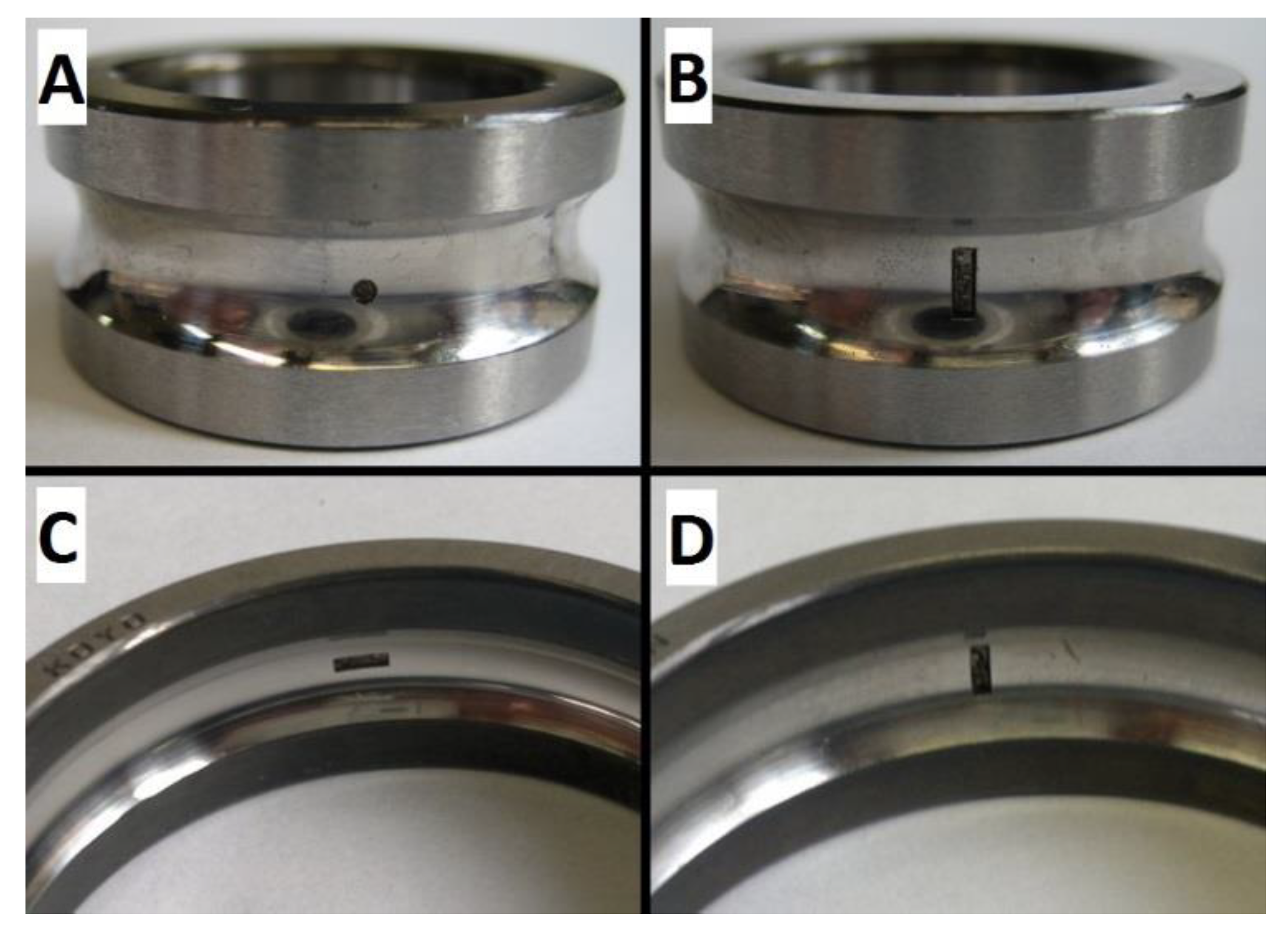
Figure 1. Experimental test rig.
Electronics 11 03885 g001
Figure 2. Close-up photos of the introduced bearing damage.
Electronics 11 03885 g002
Figure 3. A pristine bearing.
Electronics 11 03885 g003
Figure 4. The overall probabilities of correct diagnoses for inner race fault via CCSM3, for each correlation number (Table A1).
Electronics 11 03885 g004
Figure 5. The Fisher criteria, provided by CCSM3, for each correlation number (Table A1).
Electronics 11 03885 g005
Figure 6. Histograms of the diagnostic features, based on the CCSM3 (correlation number is 23—Table A1) bearings in1 and p1.
Electronics 11 03885 g006
Figure 7. Histograms of the diagnostic features, based on the CCSM3 (correlation number is 23—Table A1) bearings in2 and p2.
Electronics 11 03885 g007
Figure 8. The overall probabilities of correct diagnoses for outer race diagnosis via CCSM3 for each correlation number (Table A2).
Electronics 11 03885 g008
Figure 9. The Fisher criteria for outer race diagnosis via CCSM3, for each correlation number (Table A2).
Electronics 11 03885 g009
Figure 10. Histograms of diagnostic features based on the CCSM3 (correlation number is 4, Table A2) bearings out1 and p3.
Electronics 11 03885 g010
Figure 11. Histograms of diagnostic features based on the CCSM3 (correlation number is 4, Table A2) bearings out2 and p4.
Electronics 11 03885 g011
Table 1. List of damaged bearings, with introduced damage and relative damage sizes [26].
BearingIntroduced DamageRelative Damage Size Figure
in1inner race pit damage with 1 mm diameter and depth of 0.5 mm1.20%Figure 2A
in2inner race scratch damage length of 3 mm, width of 1 mm and
depth of 0.7 mm
1.20%Figure 2B
out1outer race scratch damage along the bearing rolling direction with length of 3 mm, width of 1 mm and depth of 0.5 mm 2.23%Figure 2C
out2outer race scratch damage length of 3 mm, width of 1 mm and depth of 0.5 mm 0.78%Figure 2D
Publisher’s Note: MDPI stays neutral with regard to jurisdictional claims in published maps and institutional affiliations.

