
Hybrid Convolutional Network Combining 3D Depthwise Separable Convolution and Receptive Field Control for Hyperspectral Image Classification


Abstract
:1. Introduction
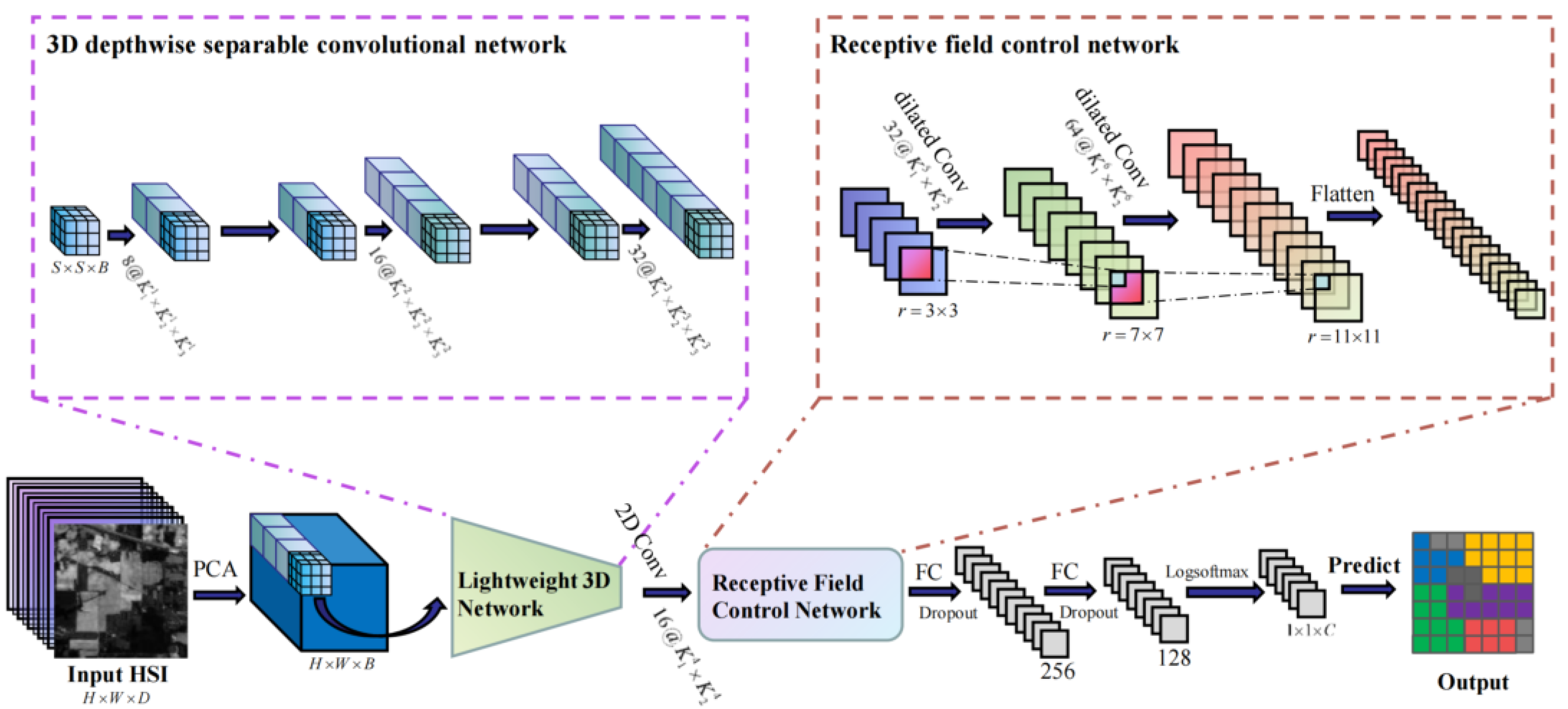
- The application of 3D depthwise separable convolution decreases the computational costs of 3D convolution. Additionally, 3D depthwise convolution can effectively capture spatial and spectral features, while pointwise convolution can extract information from adjacent spectral bands, improving the learning ability of the spectral domain.
- The receptive field control strategy is adopted. To prevent the loss of detailed information when learning multi-scale features, the receptive filed is gradually increased through dilated convolution. Moreover, the receptive field is left unchanged during 3D convolution to enhance the robustness of the model and lower the risk of overfitting.
- The experimental results show that the proposed method has a better classification accuracy in three public datasets, indicating that the model is competitive.
2. Methods
2.1. Initial Data Input and Processing
2.2. 3D Depthwise Separable Convolutional Network
2.3. Receptive Field Control Network
2.4. Fully Connected Module
2.5. Classification Result Output
3. Results
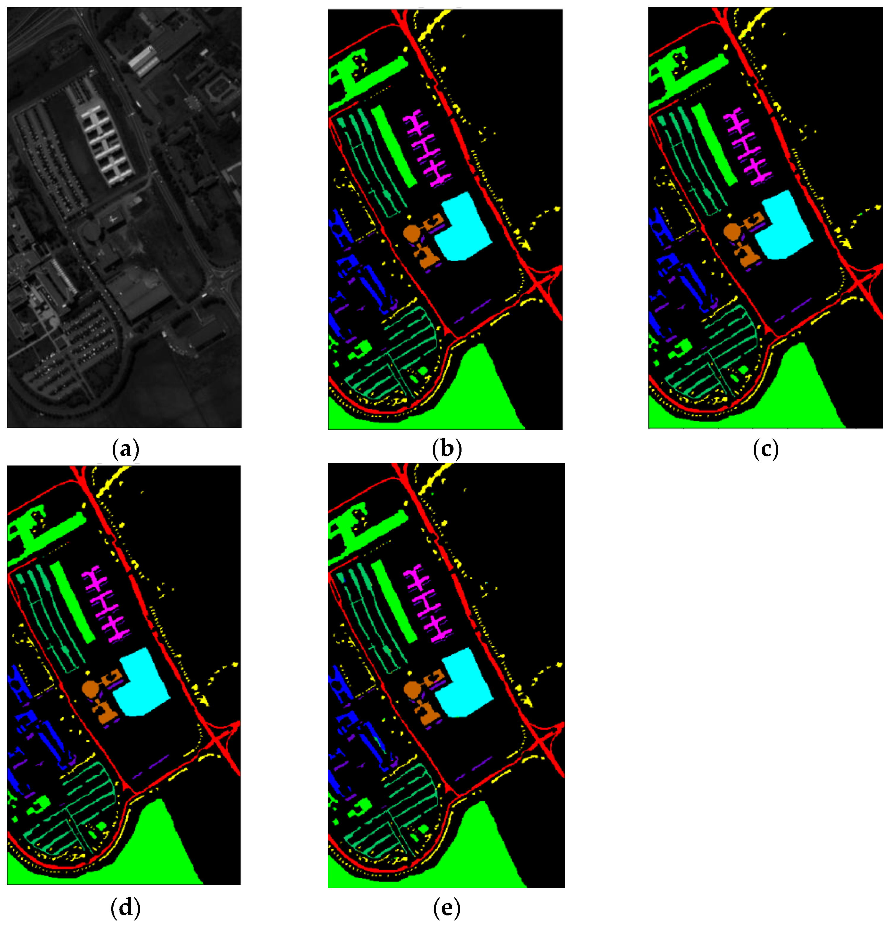
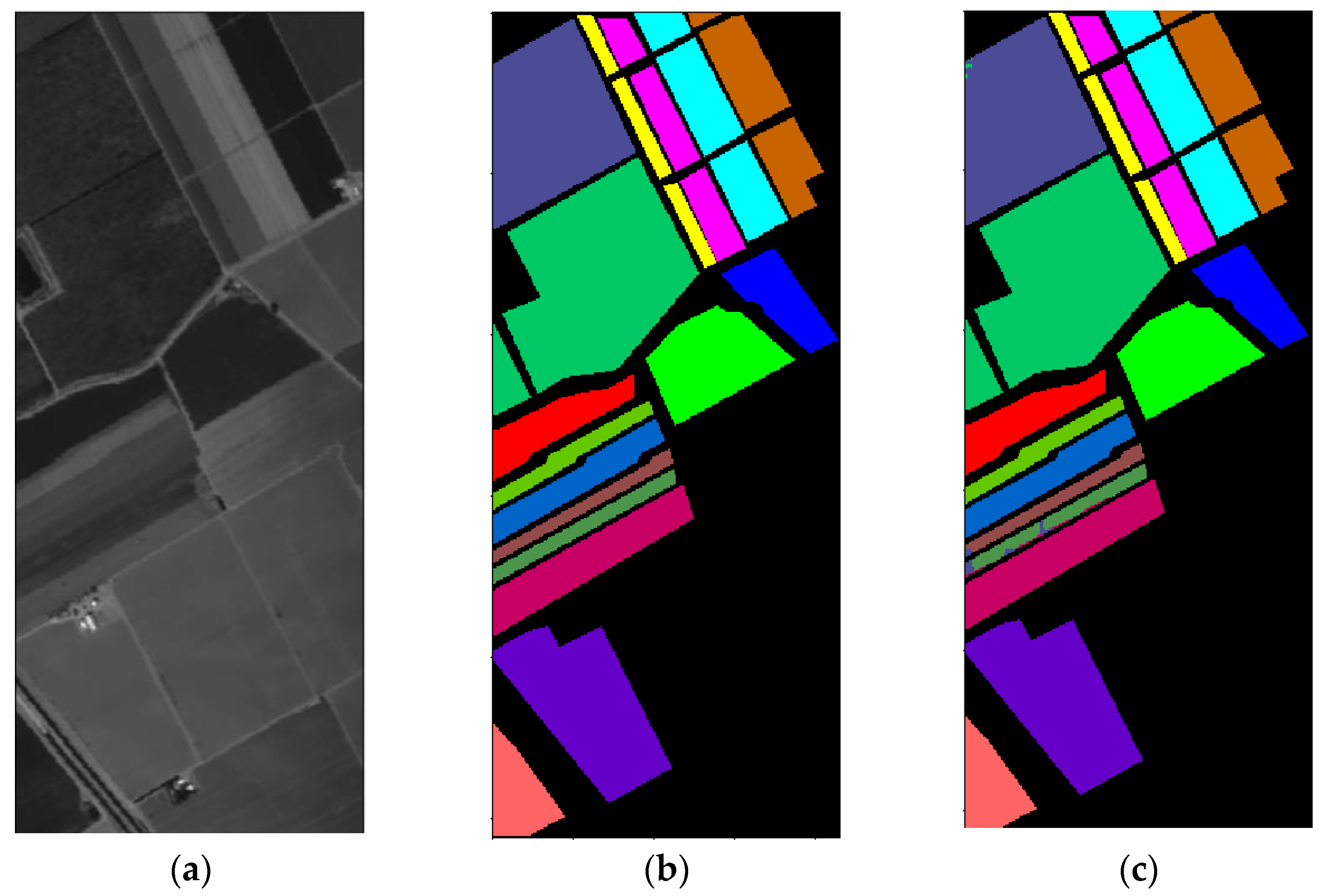
3.1. Dataset Introduction
3.2. Experimental Setup
3.3. Classification Results and Analysis
3.4. Ablation Experiments
4. Conclusions
Author Contributions
Funding
Data Availability Statement
Acknowledgments
Conflicts of Interest
References
- Zhang, H.; Zou, J.; Zhang, L. EMS-GCN: An End-to-End Mixhop Superpixel-Based Graph Convolutional Network for Hyperspectral Image Classification. IEEE Trans. Geosci. Remote Sens. 2022, 60, 5526116. [Google Scholar] [CrossRef]
- Feng, J.; Zhao, N.; Shang, R.; Zhang, X.; Jiao, L. Self-Supervised Divide-and-Conquer Generative Adversarial Network for Classification of Hyperspectral Images. IEEE Trans. Geosci. Remote Sens. 2022, 60, 5536517. [Google Scholar] [CrossRef]
- Bayramoglu, N.; Kaakinen, M.; Eklund, L.; Heikkila, J. Towards virtual H&E staining of hyperspectral lung histology images using conditional generative adversarial networks. In Proceedings of the 2017 IEEE International Conference on Computer Vision Workshops (ICCVW), Venice, Italy, 22–29 October 2017; pp. 64–71. [Google Scholar]
- Han, Y.; Shi, X.; Yang, S.; Zhang, Y.; Hong, Z.; Zhou, R. Hyperspectral Sea Ice Image Classification Based on the Spectral-Spatial-Joint Feature with the PCA Network. Remote Sens. 2021, 13, 2253. [Google Scholar] [CrossRef]
- Hu, K.; Weng, C.; Zhang, Y.; Jin, J.; Xia, Q. An Overview of Underwater Vision Enhancement: From Traditional Methods to Recent Deep Learning. J. Mar. Sci. Eng. 2022, 10, 241. [Google Scholar] [CrossRef]
- Zhou, J.; Yang, T.; Zhang, W. Underwater vision enhancement technologies: A comprehensive review, challenges, and recent trends. Appl. Intell. 2022, 1–28. [Google Scholar] [CrossRef]
- Ye, P.; Han, C.; Zhang, Q.; Gao, F.; Yang, Z.; Wu, G. An Application of Hyperspectral Image Clustering Based on Texture-Aware Superpixel Technique in Deep Sea. Remote Sens. 2022, 14, 5047. [Google Scholar] [CrossRef]
- Zhang, Q.; Zheng, E.; Wang, Y.; Gao, F. Recognition of ocean floor manganese nodules by deep kernel fuzzy C-means clustering of hyperspectral images. J. Image Graph. 2021, 26, 1886–1895. [Google Scholar]
- Li, S.; Song, W.; Fang, L.; Chen, Y.; Benediktsson, J.A. Deep Learning for Hyperspectral Image Classification: An Overview. IEEE Trans. Geosci. Remote Sens. 2019, 57, 6690–6709. [Google Scholar] [CrossRef] [Green Version]
- Wang, Q.; Meng, Z.; Li, X. Locality adaptive discriminant analysis for spectral–spatial classification of hyperspectral images. IEEE Geosci. Remote Sens. Lett. 2017, 14, 2077–2081. [Google Scholar] [CrossRef]
- Yuan, Y.; Lin, J.; Wang, Q. Hyperspectral image classification via multitask joint sparse representation and stepwise MRF optimization. IEEE Trans. Cybern. 2015, 46, 2966–2977. [Google Scholar] [CrossRef]
- Pan, B.; Shi, Z.; Xu, X. Hierarchical guidance filtering-based ensemble classification for hyperspectral images. IEEE Trans. Geosci. Remote Sens. 2017, 55, 4177–4189. [Google Scholar] [CrossRef]
- Chen, Y.; Jiang, H.; Li, C.; Jia, X.; Ghamisi, P. Deep feature extraction and classification of hyperspectral images based on convolutional neural networks. IEEE Trans. Geosci. Remote Sens. 2016, 54, 6232–6251. [Google Scholar] [CrossRef] [Green Version]
- Pan, B.; Shi, Z.; Xu, X. MugNet: Deep learning for hyperspectral image classification using limited samples. ISPRS J. Photogramm. Remote Sens. 2018, 145, 108–119. [Google Scholar] [CrossRef]
- Cheng, G.; Li, Z.; Han, J.; Yao, X.; Guo, L. Exploring hierarchical convolutional features for hyperspectral image classification. IEEE Trans. Geosci. Remote Sens. 2018, 56, 6712–6722. [Google Scholar] [CrossRef]
- Makantasis, K.; Karantzalos, K.; Doulamis, A.; Doulamis, N. Deep supervised learning for hyperspectral data classification through convolutional neural networks. In Proceedings of the 2015 IEEE International Geoscience and Remote Sensing Symposium (IGARSS), Milan, Italy, 26–31 July 2015; pp. 4959–4962. [Google Scholar]
- Jiao, L.; Liang, M.; Chen, H.; Yang, S.; Liu, H.; Cao, X. Deep fully convolutional network-based spatial distribution prediction for hyperspectral image classification. IEEE Trans. Geosci. Remote Sens. 2017, 55, 5585–5599. [Google Scholar] [CrossRef]
- Sun, H.; Zheng, X.; Lu, X. A supervised segmentation network for hyperspectral image classification. IEEE Trans. Image Process. 2021, 30, 2810–2825. [Google Scholar] [CrossRef]
- Kang, X.; Zhuo, B.; Duan, P. Dual-path network-based hyperspectral image classification. IEEE Geosci. Remote Sens. Lett. 2018, 16, 447–451. [Google Scholar] [CrossRef]
- Soucy, N.; Sekeh, S.Y. CEU-Net: Ensemble Semantic Segmentation of Hyperspectral Images Using Clustering. arXiv 2022, arXiv:2203.04873. [Google Scholar]
- Si, Y.; Gong, D.; Guo, Y.; Zhu, X.; Huang, Q.; Evans, J.; He, S.; Sun, Y. An Advanced Spectral–Spatial Classification Framework for Hyperspectral Imagery Based on DeepLab v3+. Appl. Sci. 2021, 11, 5703. [Google Scholar] [CrossRef]
- Roy, S.K.; Krishna, G.; Dubey, S.R.; Chaudhuri, B.B. HybridSN: Exploring 3-D–2-D CNN feature hierarchy for hyperspectral image classification. IEEE Geosci. Remote Sens. Lett. 2019, 17, 277–281. [Google Scholar] [CrossRef] [Green Version]
- Hamida, A.B.; Benoit, A.; Lambert, P.; Amar, C.B. 3-D deep learning approach for remote sensing image classification. IEEE Trans. Geosci. Remote Sens. 2018, 56, 4420–4434. [Google Scholar] [CrossRef] [Green Version]
- He, M.; Li, B.; Chen, H. Multi-scale 3D deep convolutional neural network for hyperspectral image classification. In Proceedings of the 2017 IEEE International Conference on Image Processing (ICIP), Beijing, China, 17–20 September 2017; pp. 3904–3908. [Google Scholar]
- Zhong, Z.; Li, J.; Luo, Z.; Chapman, M. Spectral–spatial residual network for hyperspectral image classification: A 3-D deep learning framework. IEEE Trans. Geosci. Remote Sens. 2017, 56, 847–858. [Google Scholar] [CrossRef]
- Zhu, K.; Chen, Y.; Ghamisi, P.; Jia, X.; Benediktsson, J.A. Deep convolutional capsule network for hyperspectral image spectral and spectral-spatial classification. Remote Sens. 2019, 11, 223. [Google Scholar] [CrossRef] [Green Version]
- Sun, L.; Song, X.; Guo, H.; Zhao, G.; Wang, J. Patch-wise semantic segmentation for hyperspectral images via a cubic capsule network with EMAP features. Remote Sens. 2021, 13, 3497. [Google Scholar] [CrossRef]
- Gong, H.; Li, Q.; Li, C.; Dai, H.; He, Z.; Wang, W.; Li, H.; Han, F.; Tuniyazi, A.; Mu, T. Multiscale information fusion for hyperspectral image classification based on hybrid 2D-3D CNN. Remote Sens. 2021, 13, 2268. [Google Scholar] [CrossRef]
- Ghaderizadeh, S.; Abbasi-Moghadam, D.; Sharifi, A.; Zhao, N.; Tariq, A. Hyperspectral image classification using a hybrid 3D-2D convolutional neural networks. IEEE J. Sel. Top. Appl. Earth Obs. Remote Sens. 2021, 14, 7570–7588. [Google Scholar] [CrossRef]
- Xu, H.; Yao, W.; Cheng, L.; Li, B. Multiple spectral resolution 3D convolutional neural network for hyperspectral image classification. Remote Sens. 2021, 13, 1248. [Google Scholar] [CrossRef]
- Pan, B.; Xu, X.; Shi, Z.; Zhang, N.; Luo, H.; Lan, X. DSSNet: A simple dilated semantic segmentation network for hyperspectral imagery classification. IEEE Geosci. Remote Sens. Lett. 2020, 17, 1968–1972. [Google Scholar] [CrossRef]
- Yokoya, N.; Chan, J.C.-W.; Segl, K. Potential of resolution-enhanced hyperspectral data for mineral mapping using simulated EnMAP and Sentinel-2 images. Remote Sens. 2016, 8, 172. [Google Scholar] [CrossRef] [Green Version]
- Li, Q.; Wang, Q.; Li, X. Exploring the relationship between 2D/3D convolution for hyperspectral image super-resolution. IEEE Trans. Geosci. Remote Sens. 2021, 59, 8693–8703. [Google Scholar] [CrossRef]
- Howard, A.G.; Zhu, M.; Chen, B.; Kalenichenko, D.; Wang, W.; Weyand, T.; Andreetto, M.; Adam, H. Mobilenets: Efficient convolutional neural networks for mobile vision applications. arXiv 2017, arXiv:1704.04861. [Google Scholar]
- Firat, H.; Asker, M.E.; Hanbay, D. Hybrid 3D Convolution and 2D Depthwise Separable Convolution Neural Network for Hyperspectral Image Classification. Balk. J. Electr. Comput. Eng. 2022, 10, 35–46. [Google Scholar] [CrossRef]
- Sandler, M.; Howard, A.; Zhu, M.; Zhmoginov, A.; Chen, L.-C. Mobilenetv2: Inverted residuals and linear bottlenecks. In Proceedings of the Proceedings of the IEEE conference on computer vision and pattern recognition, 2018; pp. 4510–4520.
- Jiang, Y.; Han, W.; Ye, L.; Lu, Y.; Liu, B. Two-Stream 3D MobileNetV3 for Pedestrians Intent Prediction Based on Monocular Camera. In Proceedings of the International Conference on Neural Computing for Advanced Applications, Jinan, China, 8–10 July 2022; pp. 247–259. [Google Scholar]
- Hou, B.; Liu, Y.; Ling, N.; Liu, L.; Ren, Y. A Fast Lightweight 3D Separable Convolutional Neural Network With Multi-Input Multi-Output for Moving Object Detection. IEEE Access 2021, 9, 148433–148448. [Google Scholar] [CrossRef]
- Alalwan, N.; Abozeid, A.; ElHabshy, A.A.; Alzahrani, A. Efficient 3D deep learning model for medical image semantic segmentation. Alex. Eng. J. 2021, 60, 1231–1239. [Google Scholar] [CrossRef]
- Stergiou, A.; Poppe, R. Adapool: Exponential adaptive pooling for information-retaining downsampling. arXiv 2021, arXiv:2111.00772. [Google Scholar]
- Sun, L.; Zhao, G.; Zheng, Y.; Wu, Z. Spectral–Spatial Feature Tokenization Transformer for Hyperspectral Image Classification. IEEE Trans. Geosci. Remote Sens. 2022, 60, 5522214. [Google Scholar] [CrossRef]
- Graña, M.; Veganzons, M.A.; Ayerdi, B. Hyperspectral Remote Sensing Scenes. Available online: https://www.ehu.eus/ccwintco/index.php?title=Hyperspectral_Remote_Sensing_Scenes (accessed on 5 August 2022).
- Melgani, F.; Bruzzone, L. Classification of hyperspectral remote sensing images with support vector machines. IEEE Trans. Geosci. Remote Sens. 2004, 42, 1778–1790. [Google Scholar] [CrossRef] [Green Version]
- Bai, J.; Wen, Z.; Xiao, Z.; Ye, F.; Zhu, Y.; Alazab, M.; Jiao, L. Hyperspectral Image Classification Based on Multibranch Attention Transformer Networks. IEEE Trans. Geosci. Remote Sens. 2022, 60, 5535317. [Google Scholar] [CrossRef]


| Method | IndianP | PaviaU | SalinasV | ||||||
|---|---|---|---|---|---|---|---|---|---|
| OA | Kappa | AA | OA | Kappa | AA | OA | Kappa | AA | |
| SVM [43] | 85.30 | 83.10 | 79.03 | 94.36 | 92.50 | 92.98 | 92.95 | 92.11 | 94.60 |
| 2D-CNN [16] | 89.48 | 87.96 | 86.14 | 97.86 | 97.16 | 96.55 | 97.38 | 97.08 | 98.84 |
| 3D-CNN [23] | 91.10 | 89.98 | 91.58 | 96.53 | 95.51 | 97.57 | 93.96 | 93.32 | 97.01 |
| M3D-CNN [24] | 95.32 | 94.70 | 96.41 | 95.76 | 94.50 | 95.08 | 94.79 | 94.20 | 96.25 |
| SSRN [25] | 99.19 | 99.07 | 98.93 | 99.90 | 99.87 | 99.91 | 99.98 | 99.97 | 99.97 |
| HybridSN [22] | 99.56 | 99.51 | 98.50 | 99.85 | 99.80 | 99.88 | 100 | 100 | 100 |
| 3D-Caps [26] | 90.20 | 90.15 | 93.00 | 88.34 | 84.93 | 90.14 | 88.95 | 87.74 | 94.35 |
| DSSNet [31] | 97.61 | 97.27 | 96.31 | 99.62 | 99.50 | 99.22 | 98.51 | 98.34 | 97.56 |
| EMAP-C-C [27] | 98.20 | 96.72 | 97.95 | 98.81 | 98.42 | 98.49 | 98.55 | 98.38 | 99.08 |
| MSPN [28] | 96.09 | 95.53 | 91.53 | 96.56 | 95.42 | 94.55 | 97.00 | 96.66 | 97.33 |
| SST-M [44] | 99.08 | 98.95 | 99.01 | 99.61 | 99.48 | 99.23 | / | / | / |
| LRCNet | 99.60 | 99.54 | 98.40 | 99.97 | 99.96 | 99.95 | 100 | 100 | 100 |
| Datasets | OA | Kappa | AA |
|---|---|---|---|
| IndianP | 99.31 ± 0.34 | 99.22 ± 0.38 | 98.40 ± 0.72 |
| PaviaU | 99.95 ± 0.04 | 99.93 ± 0.06 | 99.92 ± 0.04 |
| SalinasV | 99.99 ± 0.01 | 99.99 ± 0.01 | 99.98 ± 0.02 |
| Proportion of Training Samples | OA | Kappa | AA |
|---|---|---|---|
| 30% | 99.60 | 99.54 | 98.40 |
| 20% | 98.68 | 98.50 | 95.10 |
| 10% | 97.90 | 97.60 | 88.16 |
| Method | Params | Flops (MB) |
|---|---|---|
| LRCNet | 3,857,330 | 95.71 |
| HybridSN | 5,122,176 | 248.62 |
| Networks | Architecture of 3D-DW Part | OA | Kappa | AA |
|---|---|---|---|---|
| LRCNet | three 3D-DW modules | 99.60 | 99.54 | 98.40 |
| Net1 | two 3D-DW modules and one 2D-DW module | 97.16 | 96.75 | 93.75 |
| Net2 | one 3D-DW module and two 2D-DW modules | 97.09 | 96.68 | 84.29 |
| Networks | Dilation Rate | Receptive Field | OA | Kappa | AA |
|---|---|---|---|---|---|
| LRCNet | 2 | 11 × 11 | 99.60 | 99.54 | 98.40 |
| Net3 | 1 | 7 × 7 | 99.37 | 99.28 | 98.06 |
| Net4 | 3 | 15 × 15 | 98.68 | 98.49 | 97.25 |
| Net5 | 4 | 19 × 19 | 98.45 | 98.24 | 92.94 |
Publisher’s Note: MDPI stays neutral with regard to jurisdictional claims in published maps and institutional affiliations. |
© 2022 by the authors. Licensee MDPI, Basel, Switzerland. This article is an open access article distributed under the terms and conditions of the Creative Commons Attribution (CC BY) license (https://creativecommons.org/licenses/by/4.0/).
Share and Cite
Lin, C.; Wang, T.; Dong, S.; Zhang, Q.; Yang, Z.; Gao, F. Hybrid Convolutional Network Combining 3D Depthwise Separable Convolution and Receptive Field Control for Hyperspectral Image Classification. Electronics 2022, 11, 3992. https://doi.org/10.3390/electronics11233992
Lin C, Wang T, Dong S, Zhang Q, Yang Z, Gao F. Hybrid Convolutional Network Combining 3D Depthwise Separable Convolution and Receptive Field Control for Hyperspectral Image Classification. Electronics. 2022; 11(23):3992. https://doi.org/10.3390/electronics11233992
Chicago/Turabian StyleLin, Chengle, Tingyu Wang, Shuyan Dong, Qizhong Zhang, Zhangyi Yang, and Farong Gao. 2022. "Hybrid Convolutional Network Combining 3D Depthwise Separable Convolution and Receptive Field Control for Hyperspectral Image Classification" Electronics 11, no. 23: 3992. https://doi.org/10.3390/electronics11233992
APA StyleLin, C., Wang, T., Dong, S., Zhang, Q., Yang, Z., & Gao, F. (2022). Hybrid Convolutional Network Combining 3D Depthwise Separable Convolution and Receptive Field Control for Hyperspectral Image Classification. Electronics, 11(23), 3992. https://doi.org/10.3390/electronics11233992