1. Introduction
The last decade has witnessed the increasing popularity of the Internet of Things (IoT) applications, in which physical devices connect with each other in high speed, low latency, and flexible ways. The IoT aims to achieve the goal of the interconnection of everything in industry, power systems, smart cities, and other fields [
1]. In the train of such a tendency, the IoT cyber security of modern power systems has drawn increasing attention in recent years. With the amount connections between physical devices, perceiving cyber-attacks becomes a difficult task. Recent studies have begun to focus on cyberattack perception issues. Lallie et al. [
2] proposed an adapted attack graph method to refine cyberattack perception. Liang et al. [
3] established optimal attack models for different cyber-topology attack scenarios, and a metaheuristic optimization algorithm was proposed thereafter. Meanwhile, in Ref. [
4], Zhang et al. designed a cyber-attack detection system, which was established on the concept of defense-in-depth, to enhance the cyber security of cyber–physical systems (CPSs). The dependence of the IoT cyber–physical system on information systems continues to increase, which highlights the importance of cyber security in the operation of the system.
Cyber-attacks in the context of the IoT has a significant influence on cyber–physical power systems (CPPSs). With the advancement of digital substations, the risks to IoT power systems risks will result in an era dominated by information-based risks. Many cyber-attack have happened in practice: in 2015, the Ukrainian blackout event was caused by a BlackEnergy cyber-attack, which caused the grid energy management system to fail. The Stuxnet cyber-attack also significantly affected the Iranian nuclear power plant SCADA system, which laid too much burden on relevant security researchers [
5]. Choraś et al. [
6] proposed a machine learning-based technique to model behaviors and detect cyber-attacks. Meanwhile, Xin et al. [
7] concluded that system operations become seriously vulnerable to line outages and failures if cyber–physical attacks occur.
Many fault diagnosis methods have been addressed in system fault detection. Different evaluation methods have been discussed for assessing the security of cyber–physical systems. Li et al. [
8] proposed an enhanced IoT CPS security model, via which different cyber-topology attack scenarios can be recognized and classified. In [
9], a risk assessment method was presented by Liu et al. to evaluate the cyber security issues with the aid of customized protection module.
On the other hand, Bi et al. [
10] described the relationship between the context, the attack, the degree of vulnerability, and the network flow, which was proven to reflect the state of IoT CPS security. In [
11], an IoT network security situation awareness model was designed by Xu et al. to enhance the reasoning ability of an ontology model. Xiao et al. [
12] realized the online security assessment of the power grid via situation awareness technology. However, this type of method is not suitable for the real-time measurement of power grids [
13,
14]; when the information obtained by the state estimation is not accurate and comprehensive enough, this will cause a power grid dispatch center response delay and even ultimately damage to the operational stability of the power system [
15].
Jinjie et al. [
16] analyzed the situation of network topology being tampered with based on graph theory knowledge. In [
17,
18], two effective cyber-attack schemes for remote control units (RTUs) were proposed by Lallie et al. and Wang et al., respectively. Meanwhile, a method was proposed based on an improved attack graph to evaluate the hazard of cross-space cascading faults in cyber–physical power systems [
19,
20]. Zhu et al. [
21] underlined the comparison requirement in a broader range of settings, which provided promising suggestions for further work.
At present, the research on the identification methods of network attacks on the grid side mainly focuses on the identification of malicious data injection, and the coverage of attack types is insufficient. Amir et al. [
22] introduced a method to detect FDIAs targeting the AGC system by developing a stochastic unknown input estimator. The datasets in attack detection rely on the collection of abnormal traffic or vulnerability data [
23] and multi-source network data information fusion [
24]. The collection of the measured data considers single factors to analyze the overall operational state of the system, while the information fusion has the associated problems of the weak correlation between various elements and difficult data fusion, so it lacks mature and effective methods [
25]. Recently, machine learning-based technologies were studied by Benisha et al. [
26]., and Tahir et al. [
27] proposed a false data injection attack detection with an adaptive distributed sampling sequence, which can improve detection efficiency while ensuring robustness; however, data fusion was processed to train a cyber-attack detector more effectively. To achieve better efficiency, ensemble learning techniques are proposed in attack detection.
Ensemble learning techniques can achieve higher accuracy and efficiency by improving the machine learning performances of diverse base learners. Ensemble learning methods train multiple base learners to obtain improved performance and become better at transferring information than each diverse base learner [
28]. Meanwhile, the base learner algorithms result in high variance, high bias, and low accuracy. The ensemble learning algorithm usually chooses three main ensemble methods: bagging, boosting, and stacking. Several studies have shown that ensemble models often achieve higher accuracy than single machine learning models [
29]. The fundamental idea behind ensemble learning is the recognition that machine learning models have certain limitations and can make errors. Hence, ensemble learning aims to improve abnormal identification performance by adjusting the weight coefficient of multiple base models. Ensemble methods can limit the variance and bias errors associated with single machine learning models; for example, bagging reduces variance without increasing the bias, while boosting reduces bias [
30,
31]. Overall, ensemble classifiers are more robust and perform better than the individual ensemble learner. These methods have resulted in the promotion of security studies of CPPSs. Notwithstanding, the existing methods above mainly focuse on single-source data scenarios in IoT CPSs because it is difficult to trace the abnormality from physical faults and cyber-attack accurately. Meanwhile, research on multi-source heterogeneous data scenarios, which is an inevitable trend for IoT CPSs, is still lacking. Motivated by such a challenge, the main contributions of this paper are concentrated upon three aspects: (1) A hierarchical structure model of consequences under typical attack types was built and the effects of the abnormal behaviors were quantified. (2) Message data collected under different cyber-attacks was fitted by a novel ensemble learning algorithm (ELA) to identify anomalies, including power side data and information side status. (3) The security value and its probability under different cyber-attacks were determined by the combination of the feature matching method and ensemble learning algorithm. Aiming at the abnormal behaviors of cyber–physical power systems, a method to identify different attack types and physical faults is proposed to provide system situations through the proposed algorithm.
2. System Abnormal Behaviors in the IoT CPPS Hierarchical Structure
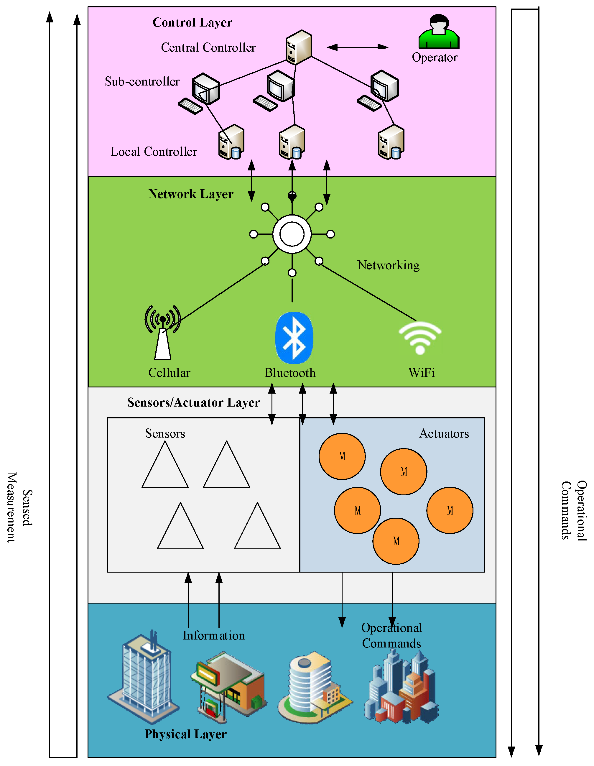
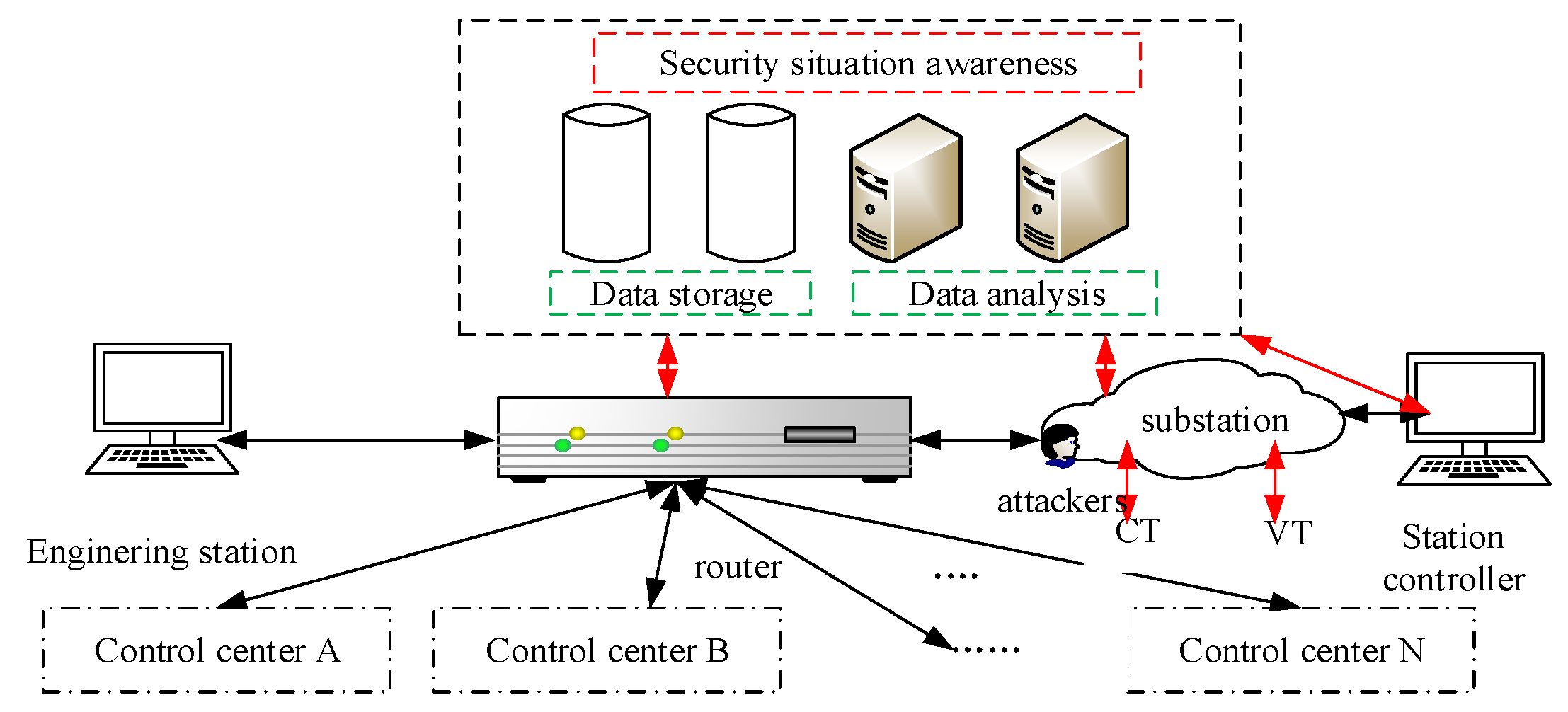
Figure 1 shows the typical architecture of an IoT CPPS [
32,
33], which includes the physical layer, sensor/actuator layer, network layer, control layer, and information layer.
Unlike the other layers, the network layer penetrates through the entire CPPS from bottom to top [
34]. Specifically, the measurement data are delivered from sensors to control units. By contrast, the operation commands are delivered from control units to actuators. Cyber-attacks in an IoT CPPS usually interfere with the normal communication between the information layer and the physical layer, which affects the information layer, causing it to send the wrong instructions to the physical layer.
The cyber-attack first occurs in the information layer. As the abnormal attack behaviors mentioned are inconsistent with the characteristics of the data set, the consequences on the information side are difficult to distinguish. For example, network flow, protocol, and business abnormality will cause the information side probe to detect a sudden change in the network flow.
Table 1 describes six typical types of abnormal attack behaviors.
According to the above mentioned six typical CPS cyber-attacks and abnormal message, the type of attack is classified according to “CIA”, with “C” representing confidentiality, “I” referring to integrity, and “A” denoting availability.
(a) “A” is for the purpose of destroying the available communication information:
- (1)
Denial-of-service attack.
A denial-of-service attack is a type of resource exhaustion attack. It uses the defects of network protocol/software or sends many useless requests to exhaust the resources of the attacked object (such as its network bandwidth), so that the server or communication network cannot provide normal services. DoS attacks can be generally divided into the following four categories: ① using protocol vulnerabilities to attack (such as in a SYN flood attack); ② using software defects to attack (such as in an OOB attack, teardrop attack, land attack, IGMP fragment packet attack, etc.); ③ sending a large number of useless requests to occupy resources (such as in an ICMP flood attack, connection flood attack, etc.); and ④ a blocking buffer spoofing attack (such as an IP spoofing DoS attack):
Abnormal port scans include ICMP scanning, 3389 external scanning, vnc scanning, etc. For example, the Windows system prohibits 135, 137, 138, 139, 445, 3389, and other high-risk ports vulnerable to malicious attacks as service ports.
(b) “C” is to destroy the confidentiality of information.
- (3)
Violent cracking.
Violent cracking includes SSH brute force cracking, FTP brute force cracking, etc., and refers to the most widely used attack techniques, with hackers using the password dictionary to guess the user’s password by employing exhaustive methods.
(c) “I” is to destroy data integrity.
- (4)
Network flow anomaly.
Network flow anomalies includes abnormal directions, sizes and types of network flow:
Abnormal protocols include message header format exception, the length of the format exception, and control domain format exceptions, etc.
- (6)
Abnormal business.
The cumulative number of remote-control trips exceeds the limit, and the interval value in terms of transmission times exceeds the limit; thus, the telemetry information exceeds the limit.
It is difficult to identify abnormal attack behavior on the data of information side. The abnormal information behavior propagates to the physical layer, which affects the stability of the frequency, the voltage values of the buses, and the current values of flexible loads. In this paper, the flexible loads are considered to be interruptible loads and transferable loads. Considering the constraints of power supply interruption capacity and times, the model of providing power for interruptible load is as follows:
where
is the power of interruptible load
j at time
t,
is the upper reserve capacity of interruptible load
j at time
t,
and
are the minimum and maximum values of interruptible load
j, respectively,
is the collection of interruptible loads, and
is the state variable of interruptible load
j at time
t. If
= 1, this indicates that the standby capacity of load
j at time
t is interruptible; otherwise, if the
= 0, this indicates that it is not interruptible.
is the statistical time set, and
is the maximum number of interruptions allowed for interruptible load
j.
The power consumption of the transferable load can be flexibly adjusted, while the total power consumption in a dispatching cycle is unchanged. The model is as follows:
where
is the power consumption of the transferable load
k at time
t,
and
are the minimum and maximum values of transferable load
k, respectively,
is a collection of transferable loads,
is the adjusted capacity of the transferable load
k at time
t, and
is the state variables of the transferable load
k at time
t.
The flexible loads have time variable and stochastic characters. The probability density function of the flexible loads can be described as:
where
is the active power of the flexible load,
is the average value of the active power in several dispatching cycles, and
is the standard deviation of active power.
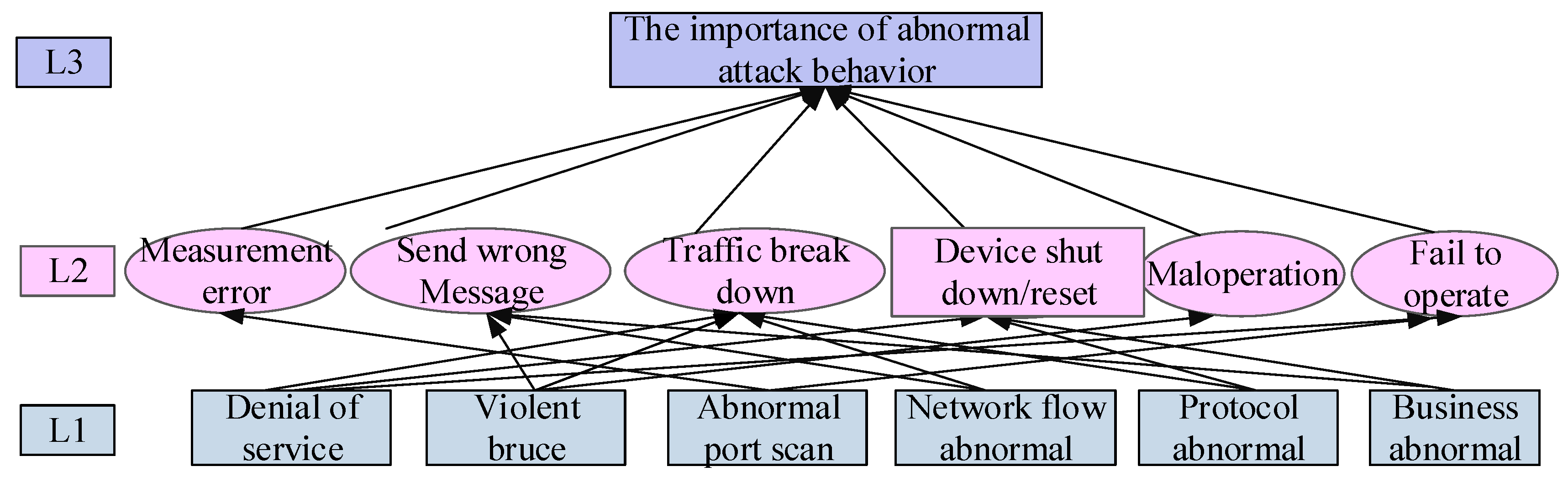
Referring to the aforementioned abnormal attack behaviors, the hierarchy of abnormal consequences is shown in
Figure 2.
The attacker can obtain the port number through the vulnerability scanning device. After obtaining the port number, the attacker can use the operating system and the device memory vulnerability to log in through the Xshell software and connect with the device IP, so that the attacker can invade the editing interface and execute the attack instructions. The attacker can tamper with the instructions of the master station to attack the stability control device in the execution station, thus affecting the power side.
Table 2 shows different abnormal behaviors and the caused possible maloperations.
3. Feature Matching Method Based on Cyber–Physical Cooperation
The cyber-attacks and fault events targeting the power system may cause abnormal phenomena on the user side. When the training data is sufficient, the gradient decision tree is used to detect the abnormality of the power system. Therefore, the current research has the problem of whether the abnormal phenomenon is caused by network attacks or failures. For example, certain common faults in a power system, such as different phase-to-phase short-circuit faults or offline faults, may cause the system to fail to operate. Meanwhile, network attacks such as man in middle attacks and denial of service attacks may cause system maloperation. All failures caused by cyber-attacks and physical faults are classified as abnormal phenomena.
To analyze whether the abnormal phenomenon is caused by a network attack or a fault, a feature sequence matching method is proposed based on cyber–physical cooperation. The causes of abnormal phenomena cannot be analyzed from the section data alone; the state transition process should be also considered. Taking denial of service (DoS) attacks as an example, the consequences caused by a DoS attack are similar to the communication delay in the system under normal conditions. How to extract features from the process of state transition to trace the causes of abnormal phenomena is the subject to be analyzed. Therefore, a feature sequence matching method was used for different abnormal phenomena to trace the cause.
3.1. Establish a State Transition Matrix
The physical elements are collected from the SCADA (Supervisory Control and Data Acquisition) system, which can reflect the operating process on the physical side. The information data mainly includes network traffic changes, log records of commands, modification records of the master station, etc. The information data mainly represents the network, protocol, and system, etc., so as to reflect the abnormal phenomena. To establish the state transition matrix, various physical elements and information data are handled to cooperate with the cyber–physical data.
Firstly, to discretize the physical analog data, the specific method is to discretize the continuous value into a value that can be used to represent the anomaly states. The advantage is that the data fluctuation caused by a small disturbance can be ignored, and only the abnormal change in the system state needs to be focused on. Considering that large disturbances, such as a frequency stability problem after line failures, the numbers impact little on the simulating results. Therefore, our specific aim was to discretize the continuous value into the a value that can be used to represent the voltage state, current state, and frequency state. The advantage of this process is that the data fluctuation caused by small disturbances can be ignored, and only the change in the system state needs to be focused on when large disturbances occur, which can be easily handled in the training and learning process. Thus, the physical measurement data includes the bus voltage, line current, system frequency, and control signals such as relay protection device action records and security control records.
3.1.1. Voltage Value Processing Method
The setting of the voltage rating generally involves certain standards according to different equipment. The equipment generally operates under the rated voltage value Un, so it is discretized as a judgment of voltage level. The measured voltage value is converted into a standard unit value. If the measured voltage value U ≤ 0.9Un, the discretized voltage state SU is described as 0. If 0.9Un < U ≤ 1.1Un and the discretized voltage state SU is described as 1. Otherwise, if U > 1.1Un, the discretized voltage state SU is described as 2.
3.1.2. Current Value Processing Method
The line current processing method is when the measured current values of multiple loads are compared with the current values in the steady state Is. The sharp fluctuation in the measured current can be regarded as abnormal. The measured current value is converted into a standard unit. If the measured current value I ≤ 0.9Is, the discretized current state SI is described as 0. If 0.9Is < I ≤ 1.5Is and the discretized current state SI is described as 1. Otherwise, if I > 1.5Is, the discretized current state SI is described as 2.
3.1.3. Frequency Processing Method
A fluctuation in the frequency between 0.996 and 1.004 of the rated frequency value fn is considered normal, while a fluctuation below 0.996fn or above 1.004fn is abnormal. Therefore, the frequency can be divided into three levels, as in the case of the voltage value processing method. If the measured frequency value f ≤ 0.996fn, the discretized frequency state Sf is described as 0. If 0.996fn < f ≤ 1.004fn and the discretized frequency state Sf is described as 1. Otherwise, if f > 1.004fn, the discretized frequency state Sf is described as 2.
3.1.4. Information Processing Method
Since the information values are originally discrete quantities, it is necessary to convert the event contents into numerical values.
The development process of each event can be represented by the system state transition process with a subscript. When an event occurs, an event state transition table can be obtained and each state can be numbered. After discretization, the states of each physical measurement or information value are limited, so the total number of the transition table is also limited. In the state transition table, the features can be extracted from the state transition process to represent the anomaly of this event.
Therefore, the state transition table
can be expressed
, which can be shown as follows:
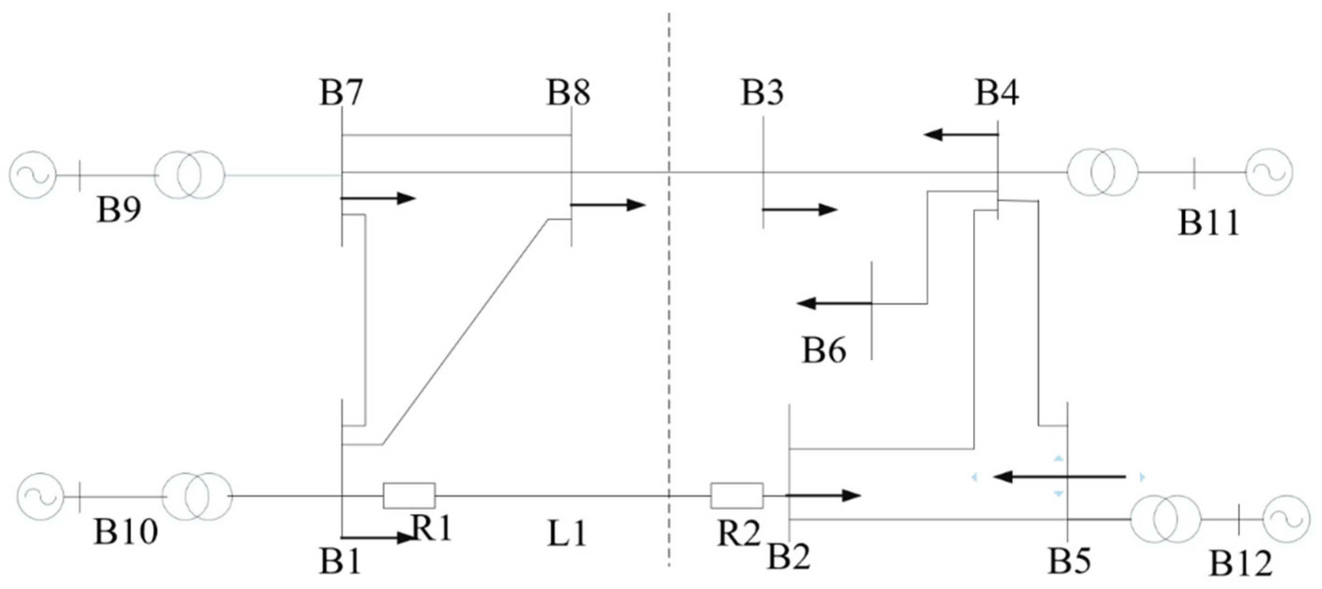
In the horizontal direction of , t is the record time, vn is the measured voltage value in node n, in is the measured voltage value in node n, switchn is the switch state in node n, and commn is the measured information value in the order of n.
Since the record discrete information value is inconsistent in the time dimension with the physical values, it is necessary to make up the values in the same time dimension. Thus, the event state transition table can be used to facilitate the analysis of change during the state transition process.
3.2. Feature Extraction during the State Transition Process
When an abnormal phenomenon occurs, there is no operational difference on the physical side, and it is difficult to distinguish between physical faults and cyber-attacks. Due to the various processes of the system state transition among different events, the extracted feature sequence will also be different. Thus, based on cyber–physical cooperative detection, the real cause of the abnormal phenomenon can be traced and the abnormal phenomenon can be classified.
Through the generation of the event state transition sequence, the characteristic events on the information side can help distinguish the types of cyber-attack and physical faults. For the preset event simulations, the feature sequences that meet the preset possibility degree are extracted from the event sequence set, and the possibility degree related to the feature sequences is formed from the preset event. Among them, the feature sequences corresponding to different possibility degrees will be different for different events. Through the idea of sequence matching, i.e., by comparing whether the sequence of unknown events contains the same sequence as the feature events extracted from a certain type of event, the unknown events are classified.
Abnormal identification can be used to analyze an abnormal behavior through the preset feature sequences. If the abnormal identification method traverses the database to detect the difference, the efficiency is slow. Therefore, to improve the accuracy and speed of identification, the ensemble learning algorithm is proposed for abnormality identification.
4. Abnormality Identification Based on the Ensemble Learning Algorithm
The machine learning solution process can be regarded as looking for a learning model with a good generalization ability and robustness in in terms of classification, but it is not easy to find an appropriate model in different situations. Therefore, as a combinatorial learning method, the ensemble learning algorithm can not only form an excellent combinatorial model by combining multiple single models, but it can also design flexible strategies for specific machine learning problems to obtain more useful solutions.
4.1. Ensemble Learning Algorithm for Anomaly Label Classification
Ensemble learning is the combination of several base machine learning learners to form a model with a smaller variance, smaller deviation, or better classification prediction effect. The ensemble learning algorithm can summarize the selection of base learners, model training, and model combination in integrated learning. In a CPPS, abnormality identification accuracy can be improved by an ensemble learning algorithm when considering the training of multiple sub-learners.
4.2. Selection of Base Learners
To guarantee classification accuracy in ensemble learning, certain algorithms are introduced as base learner candidates: the decision tree (DT), radial basis function (RBF), backward propagation (BP), least square support vector machine (LSSVM), and extreme learning machine (ELM) algorithms, as shown in
Table 3.
Since ensemble learning has a diversity property, the characteristics of its different algorithms can be different. Theoretically, to improve the diversity of the ensemble learning model, the number of base learners should be large. Such a preference, however, is opposed to computational situations in practice. Thus, a tradeoff should be considered according to practical requirements. Generally, the error of the ensemble model is related to both the accuracy and the ambiguity of the base learners. In other words, the performance of the ensemble model has a strong correlation with the accuracy or ambiguity of the base learners. Therefore, DT, RBT, and ELM base learners were selected from five candidate datasets in the ensemble learning algorithm.
4.2.1. Select Decision Tree (DT) as a Base Learner
In the DT method, a classification tree and a regression tree are involved. The Gini index can be defined as:
which is used to determine the order of the internal nodes. In the above equation,
D is the dataset,
gini(
Dk) is the Gini index of the
k-th class in
D, and
is the proportion of the
i-th class. To feature
k in
D, the
Gini index can be expressed as:
where
K is the class amount, |
Dk| is the number of the
k-th class, and |
D| is the sample amount.
When all the features have been sorted by the Gini index, a complete classification tree can be easily established via arranging all the features in sequence.
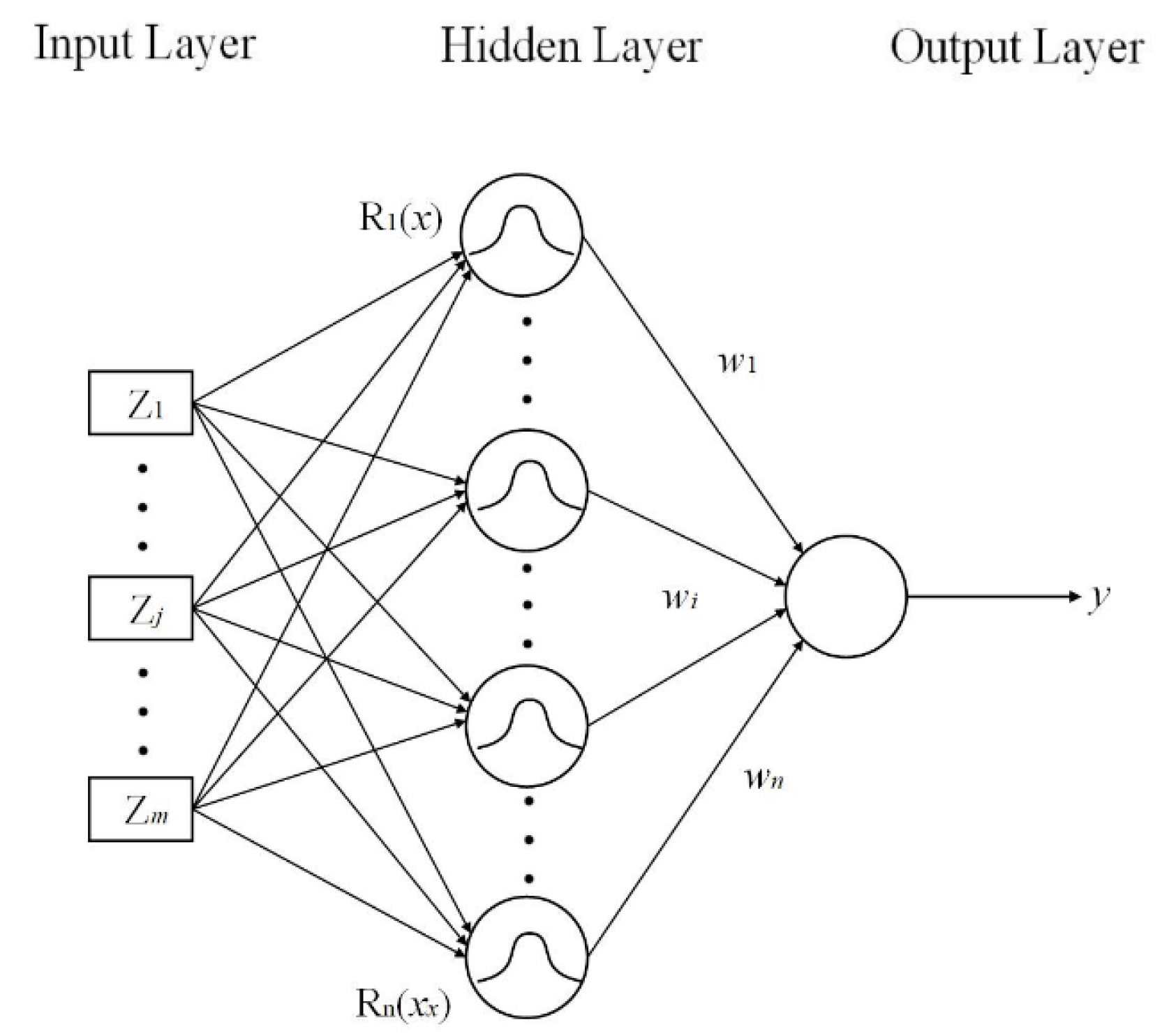
4.2.2. Select Radial Basis Function (RBF) as a Base Learner
The RBF neural network is designed using radial basis functions, and there are no local minimum points and slow learning rates, as shown in
Figure 3. The Gaussian function is used as the kernel function in the hidden layer nodes, which can be written as:
where
is the
k-th sample vector;
is the center of the
i-th hidden layer neuron;
is the variable of the hidden layer node
; and
is the norm.
The output value of the network is:
where
is the output value, and
is the network weight between the hidden layer nodes and the output layer nodes.
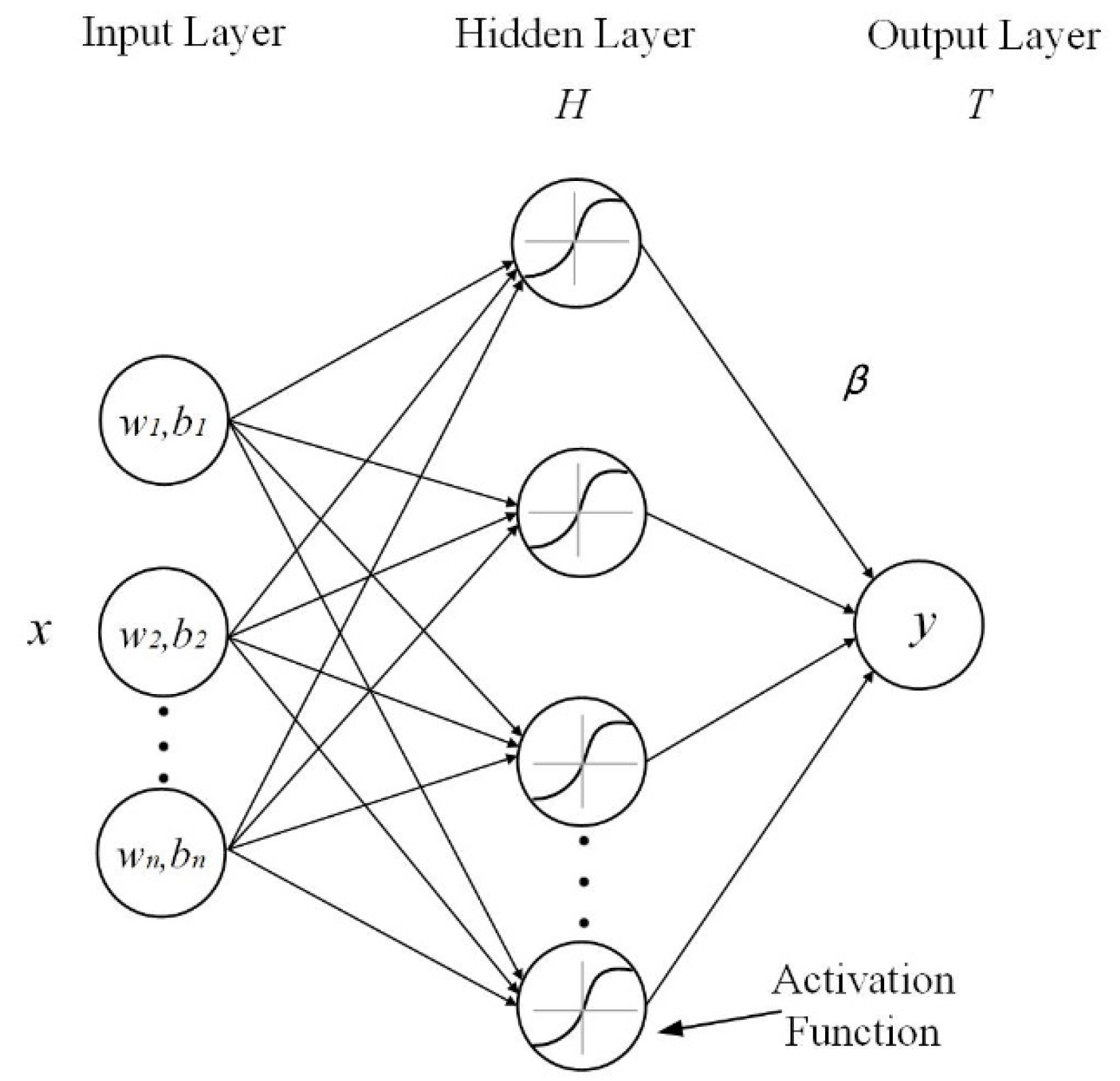
4.2.3. Select Extreme Learning Machine (ELM) as a Base Learner
Compared to the RBF algorithm, which features an iterative parameter generation process, ELM, which instead features a random parameter generation process, has a much faster training speed. The structure of ELM is shown in
Figure 4.
The mathematical relation can be expressed as:
where
H denotes the hidden layer output matrix,
β represents the output weight vector connecting hidden layer and output layer, and
T is the target output matrix. In practice, the output weight vector
β can be solved by
, where
is the Moor–Penrose generalized inverse of
H.
4.3. Basic Learner Combination under Ensemble Learning
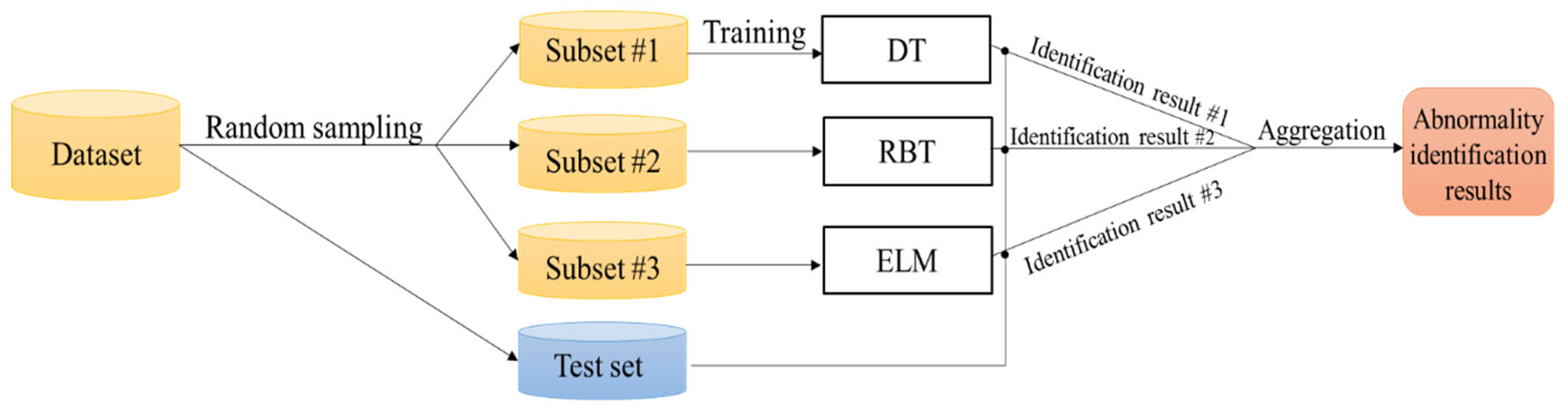
Ensemble learning for abnormality identification is achieved via the following steps. (1) The training subset is generated by randomly sampling the dataset, which can effectively reduce the training time consumption; (2) each subset is then input into each algorithm (DT, RBT, ELM) correspondingly, which ensures that the algorithm can comprehensively learn data characteristics; (3) the input of the test set into each model will then provide the identification results; (4) lastly, the results are aggregated to obtain the final abnormal identification results. The entire processes above can be visualized as
Figure 5 illustrates.
4.4. Abnormality Identification under Ensemble Learning
The ensemble learning process to identify attack behaviors can be described as follows.
Firstly, the weight distribution of training data is initialized. The initial weight
of the data set
under the machine learning algorithm is divided by the average value:
where
N is the size of the data set
,
.
In the experiment, the characteristic values of the network sample data are time stamp, message length, source, and destination address, source and destination port, data offset, check code, message version number with the length, identifier, serial number, confirmation number, check sum, emergency pointer, voltage values, current values, frequency value, switch states, and so on. As these alarm data only contain information layer data, the power change, frequency oscillation amplitude, voltage drop value, and operation condition of the related measuring equipment caused by the information layer fault in the dataset are combined.
Secondly, the training data set are used to obtain the basic classifier with the weight distribution . , m = 1, 2,…, M. In the ELA machine learner, DT, RBF, and ELM were chosen as the three different base learners.
Then, the classification error rate
of
on the training data set is calculated, with
referring to the output, which is defined in the training date.
where
represents the type of abnormal behavior under
m-th base learner, while
is the actual type of the abnormality in the dataset.
According to the
obtained by each base learner algorithm,
is used to determine whether this part of the data set should increase the weight distribution in the next iteration.
When the weight distribution of the training data set is updated, the weight
can be written as:
where
refers to the weight updated in
,
.
is the normalization factor, which makes
become a probability distribution.
Finally, a linear combination of basic classifiers is constructed:
This shows that the smaller the classification error rate, the greater the role of the classifier in the final classifier. After that, the weight distribution of training data can be updated for the next round preparation. Equation (14) can then be written as:
In feature selection, cross-validation is used to divide the training set features, which are divided into 10 sub-training sets. Each sub-training set has been trained. It is understood that the time stamp, message length, source and destination address, source and destination port, message version, and other features in 30 sub-training sets have a significant influence on the feature identification result. Therefore, the data eigenvalues obtained from the above cross-validation are used as the dataset for ensemble learning.
It can be seen that the weight of samples misclassified by the basic classifier is increased, and the weight of samples correctly classified is reduced. Thus, the weight of the misclassified samples is enlarged by multiples, so that the misclassified samples play a vital role.
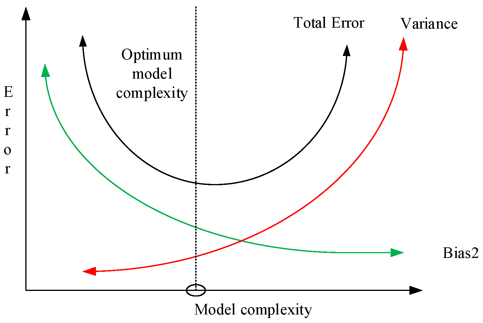
Through the combination of these measures, the bias and variance of the result can be used to identify different abnormal behaviors. An indicator RSME is used to express the quality of the established model when ensemble learning is used to solve regression problems,
where
represents the absolute difference between the real situation value and the predicted situation value under the training data of group
m,
refers to the actual situation value of the group
m, and
means the prediction value of group
m.
The model of machine learning is very dependent on data.
means the square of deviation and
refers to the complexity of the training set.
Figure 6 shows the optimum model complexity under ensemble learning. The errors in ELA are computed as (
. Generally, the more complex the model, the lower the deviation, which leads to the reduction in the total error. Therefore, the optimal model should balance the deviation and variance.


