Speed-Gradient Adaptive Control for Parametrically Uncertain UAVs in Formation

Abstract

The paper is devoted to the problem of the decentralized control of unmanned aerial vehicle (UAV) formation in the case of parametric uncertainty. A new version of the feedback linearization approach is proposed and used for a point mass UAV model transformation. As result, a linear model is obtained containing an unknown value of the UAV mass. Employing the speed-gradient design method and the implicit reference model concept, a combined adaptive control law is proposed for a single UAV, including the UAV’s mass estimation and adaptive tuning of the controller parameters. The obtained new algorithms are then used to address the problem of consensus-based decentralized control of the UAV formation. Rigorous stability conditions for control and identification are derived, and simulation results are presented to demonstrate the quality of the closed-loop control system for various conditions.

1. Introduction

Adaptation methods are widely used for various tasks involved in controlling the formation flight of unmanned aerial vehicles, such as mission formulation, target determination, trajectory formation, and ensuring movement along it, as well as control of the Unnamnned Aerial Vechicles’ (UAVs) angular position under the conditions of parametric uncertainty and characteristics of acting disturbances. Below, we consider a number of related publications from recent years.

Du et al. [1] dealt with three-dimensional (3D) unmanned aerial vehicle (UAV) path planning in a complex environment with the aim of avoiding obstacles and finding the best path to reach the target position, proposing an improved chimpanzee optimization algorithm (IChOA) based on an adaptive weight somersault foraging strategy. Sefati et al. [2] aimed to expand UAV group control concepts, including channel selection and load balancing, to improve UAV power consumption and reduce latency. Trujillo et al. [3] considered the problem of distributed control of the position of a group of UAVs to achieve the desired type of formation and avoid collisions using an adaptive convex combination of two control laws: formation control and obstacle avoidance. Two control protocols were proposed to guarantee convergence to the desired formation in a finite or given time. [4] considered the problem of collision avoidance for a swarm of UAVs and presented the results of experimental studies for a group of quadrocopters. They introduced a group-level detection and adaptation mechanism for detecting potential collisions between different groups of UAVs and restructuring the group into subgroups for better collision and deadlock avoidance. Muslimov and Munasypov [5] presented a multi-agent approach to adaptive UAV control while tracking a moving ground target. It was proposed to do this by having the UAV swarm move along a circular trajectory centered on the target. A fuzzy logic-based Model-Reference Adaptive Control (MRAC) scheme was used to cope with the uncertainty of the UAV dynamics. The approach was studied for various scenarios using full nonlinear UAV models. A strategy for searching for survivors in a dynamically changing flood zone using a group of UAVs was proposed in [6]. A robust adaptive controller was proposed for its implementation, the feasibility of which was verified by simulation in the presence of time-varying uncertainties.

Robust consensus tracking problems for a group of cloud-connected UAVs with a leader–follower formation structure in the presence of uncertainty were considered by Islam et al. [7]. The convergence performed by the Lyapunov method shows that the consensus protocol can make the states of UAV followers asymptotically track the state of the leader.

A group of agents can form a swarm using the extended Cooker–Smale (C–S) model [8]. Song et al. [9] analyzed various levels of inactivity as the degree of control efficiency for several UAVs in the flocking algorithm. In [9], a heuristic approach of adaptive inactivity was proposed, which adaptively changes the inactivity level of selected agents in accordance with their position and direction relative to the flock center. Zhou and Chen [10] used a semi-global consensus leader-following approach in which the control inputs of the leader and slave agents were bounded. Distributed static and adaptive control protocols were proposed, and adaptive updating served to avoid the use of global communication network information. The results of [10] were confirmed by both computer simulations and real flight tests employing the nanoquadrotor Crazyflie 2.1.

Ahmed et al. [11] noted that the placement of UAVs is critical when designing a network to collect data from sensors in intelligent environments, as it affects the cost, reliability, energy consumption, efficiency, and network delay. The problem was considered one of increasing the efficiency of the system by maximizing the number of serviceable sensors while using the minimum number of UAVs. Chen et al. [12] studied the multi-user UAV-enabled mobile edge computing system suffering from a jamming attack by a UAV. In this paper, reinforcement learning was applied to develop an offloading strategy to alleviate the effect caused by attack suppression that was able to comply with latency and power consumption constraints. Mahmood et al. [13] considered improving the quality of network service through the transfer of extensive computing to the mobile edge cloud and through the deployment of a UAV integrated with intelligent reflective surfaces. To achieve an effective solution to the formulated complex problem, the original optimization problem was divided into subtasks using the block coordinate method. The paper in [14] is devoted to the integration of satellite and terrestrial networks. A joint optimization design for a non-orthogonal multiple access-based satellite–terrestrial integrated network was proposed and studied in [14], and it was shown that the suggested algorithm can improve the computational efficiency of the iterative algorithm in comparison with habitual randomly generated initial points.

For networked UAVs, Güzey and Güzey [15] developed a search and tracking scheme using an adaptive hybrid grouping controller. For search, antennas were placed on at least four UAVs while keeping the system “+” in the $XY$-plane (east–west/north–south). UAVs on the abscissa axis were controlled by the difference in the signal powers of the eastern and western groups, and along the y-axis by the difference in the respective signal powers of the northern and southern groups. A backstepping controller was derived using the Lyapunov stability criteria to allow the UAV to fly in a “+” shape at a fixed altitude. Based on the example of a quadrotor troop formation, [16] proposed a number of approaches for assigning UAV targets using time optimization and gain maximization in two stages. In the first stage, urgently desired targets are selected from the detected target group using the proposed objective function. In the second, appropriate UAVs are assigned for the selected desired targets, taking into account coverage factors, adaptive limitations, and constraints.

The problem of cooperative control of a UAV group with finite-time orientation under conditions of external disturbances and parametric uncertainty was considered by Han et al. [17]. Using a quaternion model of UAV dynamics, a non-singular sliding mode terminal surface was constructed for the event-triggered controller. An adaptive neural network was used to estimate disturbances. Simulation examples were presented illustrating the efficacy of the proposed control algorithm. Wu et al. [18] considered the problem of control over a rigid formation with fixed time for a class of nonlinear multi-agent systems with indefinite dynamics and external disturbances. To compensate for the uncertainty of the system dynamics and disturbances for a fixed time, an adaptive observer was introduced for the state and disturbances. Next, a fixed-time formation control strategy was proposed. The authors proved that the designed controller implements the boundedness of closed-system errors with a fixed time independently of the initial state based on stiffness theory and the Lyapunov approach. Results based on simulations implemented on the UE4 simulation platform confirmed the control of both a single agent and a UAV formation.

A distributed adaptive fault-tolerant formation control for heterogeneous multiagent systems with faults in the communication channel was discussed in [19], where a group of heterogeneous multi-agent systems consisting of UAVs and unmanned ground vehicles (UGVs) was considered taking into account parametric uncertainties and failures in communication channels. An adaptive fault-tolerant formation control protocol was developed that uses information about local states for each slave UAV and UGV with different gains, meaning that all slave vehicles track the dynamic trajectory of the virtual leader and simultaneously provide the specified formation in case of communication channel failures or actions due to external disturbances.

Popov et al. [20] considered the problem of forming and maintaining the formation of small satellites in near-earth projected circular orbits. In [21], a two-stage algorithm for group UAV guidance was proposed. In the first stage, a consensus algorithm was employed for decentralized multi-agent UAV control. In the second, each UAV was independently guided to the target using a modified proportional 3D guidance law.

Gamagedara and Lee [22] presented a geometric adaptive position control system for a quadrotor UAV. The thrust direction, which is critical for position tracking, was controlled irrespective of the yaw direction. Adaptation elements were introduced into the control loop to mitigate the influence of the disturbances. The efficacy of the proposed control system was illustrated both numerically and experimentally by indoor and outdoor flights. Chatterjee and Dutta [23] examined the messaging process for coordinating decisions within a fully autonomous UAV group in the overall task of Plume Wrapping, which is used to determine the shape and size of airborne hazardous materials. This is a practical problem involving a real scenario. An algorithm was proposed to ensure the correctness of operation and resistance to variable delays when receiving messages.

In [24], a fractional order and trajectory control system was proposed for several quadrotors in formation using Super Twisting Sliding Mode Control (STSMC) technology. The Lyapunov function method was employed to synthesize controllers able to compensate for the influence of parametric uncertainties and wind gusts and provide justify the stability of the control system. Three types of controllers were considered: a fixed-gain STSMC, an Adaptive Super Twisting Sliding Mode Control (ASTSMC), and a Fractional-order Adaptive Super Twisting Sliding Mode Control (FASTSMC). These were tested by UAV swarm simulation. From the authors’ simulation results, the FASTSMC method demonstrated better robustness compared to the fixed-gain STSMC and integer-order ASTSMC.

For an underactuated quadrotor, Liang et al. [25] proposed an adaptive robust hierarchical control strategy. Based on the geometric approach, the orientation error in [25] was directly defined in the tangent space of the rotation group. To eliminate the influence of uncertainties, it was proposed to use a detailed dynamic model to represent the main aerodynamic and mechanical parameters of the quadrotor, and this was used to organize direct/indirect adaptive control. The presented simulation results showed the good performance of the system based on the proposed method in terms of tracking accuracy and robustness.

In a recent paper by Zhi et al. [26], the formation control of multiple fixed-wing unmanned aircraft vehicles (UAVs) based on a virtual leader structure and subject to unknown uncertainties and disturbances was studied. A fully distributed model reference robust adaptive controller (DMRRAC) was proposed, with the aim of swiftly constructing the formation in complex situations. This approach was able to dramatically reduce reliance on UAV models and global info. Meanwhile, an adaptive projection formation operator and novel high-frequency robust term of the controller were used to guarantee that the formation system was uniformly asymptotically stable under the influences of uncertainties and disturbances, and could additionally enhance the transient performance and robustness. Validation and comparative simulations were implemented to demonstrate the proposed DMRRAC method. A platform based on ROS was used to verify the actual operability of the controller.

The problem of controlling distributed formation vertical take-off and landing (VTOL) UAVs under the action of unknown perturbations was studied in [27]. Two algorithms for distributed formation control with a hierarchical structure were developed. Methods were proposed to guarantee limited thrust, work without information about acceleration, and compensation for the influence of external disturbances.

In [28], a method was proposed to ensure the overall stability of a quadrotor-type UAV formation with significant variations in the parameters of individual UAVs. It was presumed that the desired trajectory is known only to a single UAV in the formation (“the leading UAV”). For the synthesis of local controllers, a signal-parametric adaptive control based on the passification method [29,30] was employed. For illustration, the simulation results for altitude control of a group of 25 quadrotors were shown. This result was extended to the adaptive control of spatial motion for a group of quadrotors in [31]. Tomashevich and Andrievsky [32] applied an approach of [33,34] to the synthesis of a high-order adaptive algorithm for a multi-agent system control. Quadrotor attitude control was considered as an example. To demonstrate the convergence of trajectories in a system of four agents, a laboratory quadrotor setup [35] was used.

Recent results on this topic, including adaptive and variable-structure control approaches for the problem of spacecraft group motion control, can be found in the survey by [36]. The application of an adaptive coding procedure for relative motion control of two satellites over a packet erasure communication channel with a limited transmission rate was discussed in [37]. A discrete-time adaptive controller for attitude control of a single spacecraft using reaction wheels was studied in [38].

Contrary to the habitually adopted approach, when the aircraft model is derived with the help of the Taylor linearization technique in the vicinity of the given flight conditions, the feedback linearization method is applied to the nonlinear aircraft model. A rigorous justification of this approach is obtained through the theory of flat systems; see [21,39,40,41,42,43]. The novelty of the present paper’s theory is that the uncertain mass is introduced into a linearized system, in contrast to the usual approach in which the feedback-linearized plant dynamics are described by double integrators. This makes it possible to apply adaptation methods by taking into account the presence of the unknown parameter.

The remainder of this paper is organized as follows. The point-mass model of UAV dynamics is provided in Section 2. Section 3 is devoted to the adaptive control of a single UAV. Control of a multi-agent UAVs formation is considered in Section 4, and simulation results are presented in Section 5. Section 6 presents a discussion of the obtained results and compares them with other related works. Finally, our concluding remarks and future work intentions are provided in Section 7.

2. Point-Mass Model of UAV Dynamics

In this paper, we use the following point-mass model of unmanned aerial vehicle (UAV) dynamics [44,45,46]:

$$\begin{array}{cc}\hfill & \left\{\begin{array}{c}\dot{x}=V_{g}cos\gamma cos\psi ,\hfill \\ \dot{y}=V_{g}cos\gamma sin\psi ,\hfill \\ \dot{h}=V_{g}sin\gamma ,\hfill \\ {\dot{V}}_g={\displaystyle \frac{F_{\mathrm{thrust}}-F_{\mathrm{drag}}}{m}}-gsin\gamma ,\hfill \\ \dot{\psi }={\displaystyle \frac{F_{\mathrm{lift}}sin\phi }{V_{g}mcos\gamma }},\hfill \\ \dot{\gamma }={\displaystyle \frac{F_{\mathrm{lift}}cos\phi }{V_{g}m}}-{\displaystyle \frac{gcos\gamma }{V_g}},\hfill \end{array}\right.\hfill \end{array}$$

(1)

where x, y, h are UAV translational coordinates; $\gamma$ denotes the flight-path angle; $\psi$ is the heading angle; $\phi$ is the bank angle; $V_g$ denotes the UAV ground speed; $F_{\mathrm{lift}}={\displaystyle \frac{1}{2}}{\rho }_a{V_g}^{2}S{C}_L$, $F_{\mathrm{drag}}={\displaystyle \frac{1}{2}}{\rho }_a{V_g}^{2}S{C}_D$ are the lift and drag forces, respectively; $F_{\mathrm{thrust}}$ denotes the thrust force; m is the UAV mass; g stands for the gravity acceleration constant; S is the platform area for a wing; and ${\rho }_a$ denotes the air density; finally, $C_L$ is the lift coefficient, $C_D$ is the drag coefficient, and $C_D=C_{D_0}+k_c{C}_L^2$, where $C_{D_0}$ denotes zero lift drag coefficient, $k_c$ is the induced drag factor. Following [40,47], let us adopt $u={[F_{\mathrm{thrust}},C_L,\phi ]}^{\mathrm{T}}$ as the vector of the control signals.

In [39,41,42,48], a variant of (1) is used in which the load factor is defined as

$$\begin{array}{c}\hfill n_{\mathrm{lf}}\triangleq {\displaystyle \frac{F_{\mathrm{lift}}}{mg}}\end{array}$$

and used instead of the lift coefficient $C_L$. Then, (1) takes the following form:

$$\begin{array}{c}\hfill \left\{\begin{array}{c}\dot{x}=V_{g}cos\gamma cos\psi ,\hfill \\ \dot{y}=V_{g}cos\gamma sin\psi ,\hfill \\ \dot{h}=V_{g}sin\gamma ,\hfill \\ {\dot{V}}_g={\displaystyle \frac{F_{\mathrm{thrust}}-F_{\mathrm{drag}}}{m}}-gsin\gamma ,\hfill \\ \dot{\psi }={\displaystyle \frac{n_{\mathrm{lf}}gsin\phi }{V_{g}cos\gamma }},\hfill \\ \dot{\gamma }={\displaystyle \frac{g\left(n_{\mathrm{lf}}cos\phi -cos\gamma \right)}{V_g}}.\hfill \end{array}\right.\end{array}$$

(2)

Zhi et al. [26], Wang and Xin [43] used the following variant of (2):

$$\begin{array}{c}\hfill \left\{\begin{array}{c}\dot{x}=V_{g}cos\gamma cos\psi ,\hfill \\ \dot{y}=V_{g}cos\gamma sin\psi ,\hfill \\ \dot{h}=V_{g}sin\gamma ,\hfill \\ {\dot{V}}_g={\displaystyle \frac{F_{\mathrm{thrust}}-F_{\mathrm{drag}}}{m}}-gsin\gamma ,\hfill \\ \dot{\psi }={\displaystyle \frac{n_{\mathrm{lf}}gsin\phi }{V_{g}cos\gamma }},\hfill \\ \dot{\gamma }={\displaystyle \frac{F_{\mathrm{lift}}cos\phi }{V_{g}m}}-{\displaystyle \frac{gcos\gamma }{V_g}},\hfill \end{array}\right.\end{array}$$

(3)

where the control action is defined as in (2), i.e., $u={[F_{\mathrm{thrust}},n_{\mathrm{lf}},\phi ]}^{\mathrm{T}}$.

2.1. Feedback Linearization

Models (1)–(3) ues a common approach to the design of the control algorithm, namely, the feedback linearization method, cf. [49]. This results in an equivalent linear system of the form

$$\begin{array}{c}\hfill \ddot{x}=v_1,\\ \hfill \ddot{y}=v_2,\\ \hfill \ddot{h}=v_3,\end{array}$$

(4)

where $v_1$, $v_2$, $v_3$ are virtual controls which can be uniquely converted into real ones. This approach was used in [39,40,42,43], and, appears indirectly in [26]. A rigorous justification for the applicability of this approach follows from the theory of flat systems [50,51]. It can be shown that outputs $x\left(t\right)$, $y\left(t\right)$, $h\left(t\right)$ of systems (1)–(3) are flat (in the sense of [50,51]) and that variables $V_g$, $\psi$, $\gamma$ can be expressed in terms of x, y, h and their derivatives, as well as in terms of control signals. Let the real control signals in (1) be in the form $u={[F_{\mathrm{thrust}},F_{\mathrm{lift}},\phi ]}^{\mathrm{T}}$; here, $F_{\mathrm{lift}}$ is used instead of $C_L$. Such a replacement is admissible because it follows from the seventh equation in (1) that the required value of $C_L$ can be uniquely obtained from $F_{\mathrm{lift}}$. Then, the inverse transformations of the control by dynamic feedback linearization can be obtained in the following form:

Option 1.

$$\begin{array}{cc}\hfill & F_{\mathrm{thrust}}=F_{\mathrm{drag}}+mcos\gamma \left(v_{1}cos\psi +v_{2}sin\psi \right)+msin\gamma \left(g+v_3\right),\hfill \\ \hfill & F_{\mathrm{lift}}=m\sqrt{{\left(\left(g+v_3\right)cos\gamma -sin\gamma \left(v_{1}cos\psi -v_{2}sin\psi \right)\right)}^2+{\left(v_{2}cos\psi -v_{1}sin\psi \right)}^2},\hfill \\ \hfill & \phi =arctan\left(\frac{v_{2}cos\psi -v_{1}sin\psi }{\left(g+v_3\right)cos\gamma -\left(v_{1}cos\psi +v_{2}sin\psi \right)sin\gamma }\right).\hfill \end{array}$$

(5)

Option 2.

$$\begin{array}{cc}\hfill & F_{\mathrm{thrust}}=F_{\mathrm{drag}}+m{\displaystyle \frac{\dot{x}{v}_1+\dot{y}{v}_2+\dot{h}\left(g+v_3\right)}{V_g}}\hfill \\ \hfill & F_{\mathrm{lift}}=m{\displaystyle \frac{(g+v_3)cos\gamma -(v_{1}cos\psi +v_{2}sin\psi )sin\gamma }{cos\phi }},\hfill \\ \hfill & \phi =arctan\left({\displaystyle \frac{v_{2}cos\psi -v_{1}sin\psi }{\left(g+v_3\right)cos\gamma -\left(v_{1}cos\psi +v_{2}sin\psi \right)sin\gamma }}\right)\hfill \end{array}$$

(6)

Option 3.

$$\begin{array}{cc}\hfill & F_{\mathrm{thrust}}=F_{\mathrm{drag}}+mcos\gamma \left(v_{1}cos\psi +v_{2}sin\psi \right)+msin\gamma \left(g+v_3\right),\hfill \\ \hfill & F_{\mathrm{lift}}=m{\displaystyle \frac{\left(g+v_3\right)cos\gamma -\left(v_{1}cos\psi +v_{2}sin\psi )\right)sin\gamma }{cos\phi }},\hfill \\ \hfill & \phi =arctan\left({\displaystyle \frac{v_{2}cos\psi -v_{1}sin\psi }{\left(g+v_3\right)cos\gamma -\left(v_{1}cos\psi +v_{2}sin\psi \right)sin\gamma }}\right).\hfill \end{array}$$

(7)

Note that the respective expressions for $F_{\mathrm{thrust}}$ and $F_{\mathrm{lift}}$ in all three options are equivalent.

The admissible region in the phase space of the UAV model, in which the obtained expressions (5)–(7) are defined for (1), is provided by the following inequalities:

$$\begin{array}{c}\hfill V_g>0,\left|\gamma \right|<\pi /2,\left|\phi \right|<\pi /2.\end{array}$$

(8)

Similar expressions for systems (2) and (3) can be obtained to transform the virtual control signals $v_1$, $v_2$, and $v_3$ into the real ones.

2.2. Feedback Linearization for Variable Mass m Case

The control signals in (5)–(7) are computed from the virtual controls $v_1$, $v_2$, and $v_3$ for system (4). Because Expression (4) does not contain the mass m in it, the mass change is not taken into account when virtual controls are computed. In order to take into account the influence of the mass, we can make transformations in (4)–(7) by employing the following changes in variables:

$$\begin{array}{c}\hfill m{v}_1={\overline{v}}_1,\\ \hfill m{v}_2={\overline{v}}_2,\\ \hfill m(v_3+g)={\overline{v}}_3.\end{array}$$

(9)

Then,

$$\begin{array}{cc}\hfill v_1& =\frac{1}{m}{\overline{v}}_1,\hfill \\ \hfill v_2& =\frac{1}{m}{\overline{v}}_2,\hfill \\ \hfill v_3& =\frac{1}{m}{\overline{v}}_3-g.\hfill \end{array}$$

(10)

After substituting (10) into (4), we have

$$\begin{array}{cc}\hfill \ddot{x}& =\frac{1}{m}{\overline{v}}_1,\hfill \\ \hfill \ddot{y}& =\frac{1}{m}{\overline{v}}_2,\hfill \\ \hfill \ddot{h}& =\frac{1}{m}{\overline{v}}_3-g,\hfill \end{array}$$

(11)

where ${\overline{v}}_1,{\overline{v}}_2,{\overline{v}}_3$ are the new virtual controls.

Now, the transformations to the real control signals (5)–(7) are as follows:

Option 1.

$$\begin{array}{cc}\hfill & F_{\mathrm{thrust}}=F_{\mathrm{drag}}+cos\gamma \left({\overline{v}}_{1}cos\psi +{\overline{v}}_{2}sin\psi \right)+{\overline{v}}_{3}sin\gamma ,\hfill \\ \hfill & F_{\mathrm{lift}}=\sqrt{{\left({\overline{v}}_{3}cos\gamma -sin\gamma \left({\overline{v}}_{1}cos\psi -{\overline{v}}_{2}sin\psi \right)\right)}^2+{\left({\overline{v}}_{2}cos\psi -{\overline{v}}_{1}sin\psi \right)}^2},\hfill \\ \hfill & \phi =arctan\left({\displaystyle \frac{{\overline{v}}_{2}cos\psi -{\overline{v}}_{1}sin\psi }{{\overline{v}}_{3}cos\gamma -\left({\overline{v}}_{1}cos\psi +{\overline{v}}_{2}sin\psi \right)sin\gamma }}\right).\hfill \end{array}$$

(12)

Option 2.

$$\begin{array}{cc}\hfill & F_{\mathrm{thrust}}=F_{drag}+\left(\dot{x}{\overline{v}}_1+\dot{y}{\overline{v}}_2+\dot{h}{\overline{v}}_3\right)/V_g,\hfill \\ \hfill & F_{\mathrm{lift}}={\displaystyle \frac{{\overline{v}}_{3}cos\gamma -\left({\overline{v}}_{1}cos\psi +{\overline{v}}_{2}sin\psi \right)sin\gamma }{cos\phi }},\hfill \\ \hfill & \phi =arctan\left({\displaystyle \frac{{\overline{v}}_{2}cos\psi -{\overline{v}}_{1}sin\psi }{{\overline{v}}_{3}cos\gamma -\left({\overline{v}}_{1}cos\psi +{\overline{v}}_{2}sin\psi )\right)sin\gamma }}\right).\hfill \end{array}$$

(13)

Option 3.

$$\begin{array}{cc}\hfill & F_{\mathrm{thrust}}=F_{\mathrm{drag}}+cos\gamma \left({\overline{v}}_{1}cos\psi +{\overline{v}}_{2}sin\psi \right)+{\overline{v}}_{3}sin\gamma ,\hfill \\ \hfill & F_{\mathrm{lift}}={\displaystyle \frac{{\overline{v}}_{3}cos\gamma -\left({\overline{v}}_{1}cos\psi +{\overline{v}}_{2}sin\psi \right)sin\gamma }{cos\phi }},\hfill \\ \hfill & \phi =arctan\left({\displaystyle \frac{{\overline{v}}_{2}cos\psi -{\overline{v}}_{1}sin\psi }{{\overline{v}}_{3}cos\gamma -\left({\overline{v}}_{1}cos\psi +{\overline{v}}_{2}sin\psi \right)sin\gamma }}\right).\hfill \end{array}$$

(14)

Note that the right-hand sides of (12)–(14) do not include the mass m.

3. Adaptive Control of Single UAV

3.1. Problem Statement and Control Goal

Now, we pose the following control goal: find controls for system (11) while ensuring tracking of a given trajectory under the condition of an unknown (or slowly time-varying) parameter $m\left(t\right)$, assuming that the range of its possible values is known, i.e., $\forall t:m_{min}⩽m\left(t\right)⩽m_{max}$. First, we consider the following prescribed trajectory:

$$\begin{array}{c}\hfill r\left(t\right)={[r_x\left(t\right),r_y\left(t\right),r_h\left(t\right)]}^{\mathrm{T}},\end{array}$$

(15)

where the vector function $r\left(t\right)\in {\mathbb{R}}^3$ is formed from the reference coordinates $r_x\left(t\right)$, $r_y\left(t\right)$, $r_h\left(t\right)$ along axes x, y, h, respectively. Assume that the time derivatives of $r\left(t\right)$ up to $\ddot{r}\left(t\right)$ inclusive are bounded for all $t>0$ and the derivative $\ddot{r}\left(t\right)$ is a piecewise continuous function of t.

To solve the posed problem, the following new variables are introduced:

$$\begin{array}{cc}\hfill e_{x1}& =x_1-r_x\left(t\right),e_{x2}=x_2-{\dot{r}}_x\left(t\right),\hfill \\ \hfill e_{y1}& =y_1-r_y\left(t\right),e_{y2}=y_2-{\dot{r}}_y\left(t\right),\hfill \\ \hfill e_{h1}& =h_1-r_h\left(t\right),e_{h2}=h_2-{\dot{r}}_h\left(t\right),\hfill \end{array}$$

(16)

where $x_1=x$, $x_2=\dot{x}$, $y_1=y$, $y_2=\dot{y}$, $h_1=h$, $h_2=\dot{h}$, and

$$\begin{array}{cc}\hfill y_x& ={\alpha }_x{e}_{x1}+e_{x2},\hfill \\ \hfill y_y& ={\alpha }_y{e}_{y1}+e_{y2},\hfill \\ \hfill y_h& ={\alpha }_h{e}_{h1}+e_{h2},\hfill \end{array}$$

(17)

with some ${\alpha }_x>0$, ${\alpha }_y>0$, ${\alpha }_h>0$.

We now introduce the following goal function:

$$Q_t(e_{\mathrm{xyh}},y_{\mathrm{xyh}})={\displaystyle \frac{1}{2}}{e}_{x1}^2+{\displaystyle \frac{1}{2}}{e}_{y1}^2+{\displaystyle \frac{1}{2}}{e}_{h1}^2+{\displaystyle \frac{m}{2}}{y}_x^2+{\displaystyle \frac{m}{2}}{y}_y^2+{\displaystyle \frac{m}{2}}{y}_h^2.$$

(18)

where $e_{\mathrm{xyh}}=(e_{x1},e_{y1},e_{h1})$, $y_{\mathrm{xyh}}=(y_x,y_y,y_h)$. Here, the control goal is provided by the asymptotic relation

$$\underset{t\to \infty }{lim}{Q}_t(e_{\mathrm{xyh}},y_{\mathrm{xyh}})=0.$$

(19)

With respect to the new variables from (16), system (11) has the following form:

$$\begin{array}{cc}\hfill {\ddot{e}}_{x1}& ={\displaystyle \frac{1}{m}}{\overline{v}}_1-{\ddot{r}}_x\left(t\right),\hfill \\ \hfill {\ddot{e}}_{y1}& ={\displaystyle \frac{1}{m}}{\overline{v}}_2-{\ddot{r}}_y\left(t\right),\hfill \\ \hfill {\ddot{e}}_{h1}& ={\displaystyle \frac{1}{m}}{\overline{v}}_3-g-{\ddot{r}}_h\left(t\right).\hfill \end{array}$$

(20)

Substituting the variables from (17) to (20), we obtain

$$\begin{array}{cc}\hfill {\dot{e}}_{x1}& =-{\alpha }_x{e}_{x1}+y_x,\hfill \\ \hfill {\dot{e}}_{y1}& =-{\alpha }_y{e}_{y1}+y_y,\hfill \\ \hfill {\dot{e}}_{h1}& =-{\alpha }_h{e}_{h1}+y_h,\hfill \end{array}$$

(21)

$$\begin{array}{cc}\hfill {\dot{y}}_x& ={\alpha }_x{y}_x-{\alpha }_x^2{e}_{x1}+\frac{1}{m}{\overline{v}}_1-{\ddot{r}}_x\left(t\right),\hfill \\ \hfill {\dot{y}}_y& ={\alpha }_y{y}_y-{\alpha }_y^2{e}_{y1}+\frac{1}{m}{\overline{v}}_2-{\ddot{r}}_y\left(t\right),\hfill \\ \hfill {\dot{y}}_h& ={\alpha }_h{y}_h-{\alpha }_h^2{e}_{h1}+\frac{1}{m}{\overline{v}}_3-{\ddot{r}}_h\left(t\right)-g.\hfill \end{array}$$

(22)

Equation (21) describes the internal dynamics, while (22) is used for the external dynamics. Obviously, the null dynamics of system (21) are exponentially stable [49].

3.2. Design of Main Control Loop

We take the control for the system (21)–(22) in the following form:

$$\begin{array}{cc}\hfill {\overline{v}}_1& =-\widehat{m}\left(k_x{y}_x-{\ddot{r}}_x\left(t\right)\right)+{\widehat{k}}_x{y}_x,\hfill \\ \hfill {\overline{v}}_2& =-\widehat{m}\left(k_y{y}_y-{\ddot{r}}_y\left(t\right)\right)+{\widehat{k}}_y{y}_y,\hfill \\ \hfill {\overline{v}}_3& =-\widehat{m}\left(k_h{y}_h-{\ddot{r}}_h\left(t\right)-g\right)+{\widehat{k}}_h{y}_h,\hfill \end{array}$$

(23)

where $\widehat{m}$, ${\widehat{k}}_x$, ${\widehat{k}}_y$, ${\widehat{k}}_h$ are adjustable parameters and $k_x>0$, $k_y>0$, $k_h>0$ are fixed (design) parameters.

Substituting (23) into (22), we have

$$\begin{array}{cc}\hfill {\dot{y}}_x& =-{\alpha }_x^2{e}_{x1}+\left({\alpha }_x-\frac{\widehat{m}}{m}{k}_x+\frac{{\widehat{k}}_x}{m}\right)y_x+\left(\frac{\widehat{m}}{m}-1\right){\ddot{r}}_x\left(t\right),\hfill \\ \hfill {\dot{y}}_y& =-{\alpha }_y^2{e}_{y1}+\left({\alpha }_y-\frac{\widehat{m}}{m}{k}_y+\frac{{\widehat{k}}_y}{m}\right)y_y+\left(\frac{\widehat{m}}{m}-1\right){\ddot{r}}_y\left(t\right),\hfill \\ \hfill {\dot{y}}_h& =-{\alpha }_h^2{e}_{h1}+\left({\alpha }_h-\frac{\widehat{m}}{m}{k}_h+\frac{{\widehat{k}}_h}{m}\right)y_h+\left(\frac{\widehat{m}}{m}-1\right)({\ddot{r}}_h\left(t\right)+g).\hfill \end{array}$$

(24)

Now, the following Proposition can be stated.

Proposition 1.

For system (21) and (22) with control (23) and with a known value of m, it is always possible to find values of control parameters $\widehat{m}$, $k_x$, $k_y$, $k_h$, ${\widehat{k}}_x$, ${\widehat{k}}_y$, ${\widehat{k}}_h$ such that control goal (19) is fulfilled and the closed-loop system is exponentially stable.

Proof of Proposition 1.

Take the following parameter values:

$$\begin{array}{cc}\hfill \widehat{m}{}_{\ast }& =m,\hfill \\ \hfill k_x& ={\alpha }_x,k_y={\alpha }_y,k_h={\alpha }_h,\hfill \\ \hfill {\widehat{k}}_{x\ast }& =-{\lambda }_{x}m,{\widehat{k}}_{y\ast }=-{\lambda }_{y}m,{\widehat{k}}_{h\ast }=-{\lambda }_{h}m,\hfill \end{array}$$

(25)

where ${\lambda }_x>0$, ${\lambda }_y>0$, ${\lambda }_h>0$ are arbitrarily chosen positive constants (the design parameters).

Then, substituting (25) into (24) provides us with

$$\begin{array}{cc}\hfill {\dot{y}}_x& =-{\alpha }_x^2{e}_{x1}-{\lambda }_x{y}_x,\hfill \\ \hfill {\dot{y}}_y& =-{\alpha }_y^2{e}_{y1}-{\lambda }_y{y}_y,\hfill \\ \hfill {\dot{y}}_h& =-{\alpha }_h^2{e}_{h1}-{\lambda }_h{y}_h.\hfill \end{array}$$

(26)

Take the following Lyapunov function:

$$V\left(t\right)=Q_t(e_{\mathrm{xyh}},y_{\mathrm{xyh}})$$

(27)

and calculate the time derivative of $V\left(t\right)$ along the trajectories of system (21) and (26):

$$\begin{array}{cc}\hfill \dot{V}& =e_{x1}{\dot{e}}_{x1}+m{y}_x{\dot{y}}_x+e_{y1}{\dot{e}}_{y1}+m{y}_y{\dot{y}}_y+e_{h1}{\dot{e}}_{h1}+m{y}_h{\dot{y}}_h.\hfill \end{array}$$

(28)

Grouping the terms for the x, y, and h axes in (28) results in

$$\begin{array}{c}\hfill \dot{V}={\dot{V}}_x+{\dot{V}}_y+{\dot{V}}_h,\end{array}$$

(29)

where

$$\begin{array}{cc}\hfill {\dot{V}}_x& =e_{x1}{\dot{e}}_{x1}+m{y}_x{\dot{y}}_x,\hfill \\ \hfill {\dot{V}}_y& =e_{y1}{\dot{e}}_{y1}+m{y}_y{\dot{y}}_y,\hfill \\ \hfill {\dot{V}}_h& =e_{h1}{\dot{e}}_{h1}+m{y}_h{\dot{y}}_h.\hfill \end{array}$$

(30)

Below, only the expression for ${\dot{V}}_x$ is considered; however, transformations for ${\dot{V}}_y$, ${\dot{V}}_h$ can be made similarly. Making substitutions of expressions for derivatives, we obtains

$$\begin{array}{c}\hfill {\dot{V}}_x=e_{x1}\left(-{\alpha }_x{e}_{x1}+y_x\right)+m{y}_x(-{\alpha }_x^2{e}_{x1}-{\lambda }_x{y}_x)=-{\alpha }_x{e}_{x1}^2+\left(1-m{\alpha }_x^2\right)e_{x1}{y}_x-m{\lambda }_x{y}_x^2.\end{array}$$

(31)

It can be easily seen that ${\dot{V}}_x$ can be represented as a following quadratic form

$$\begin{array}{c}\hfill {\dot{V}}_x={{\eta }_x}^{\mathrm{T}}{H}_x{\eta }_x,\end{array}$$

(32)

where vector ${\eta }_x={\left[e_{x1}{y}_x\right]}^{\mathrm{T}}$ and matrix

$$\begin{array}{c}\hfill H_x=\left[\begin{array}{cc}-{\alpha }_x& 0.5\left(1-m{\alpha }_x^2\right)\\ 0.5\left(1-m{\alpha }_x^2\right)& -m{\lambda }_x\end{array}\right]\end{array}$$

(33)

are introduced.

Matrix $H_x=H_x^{\mathrm{T}}$ is negative definite if its first angular minor is negative and its second is positive. In our case, the first minor ${\Delta }_1=-{\alpha }_x<0$, and the second should satisfy the inequality

$$\begin{array}{c}\hfill {\Delta }_2=m{\alpha }_x{\lambda }_x-0.25{\left(1-m{\alpha }_x^2\right)}^2>0.\end{array}$$

(34)

We can represent inequality (34) in the following form:

$$\begin{array}{c}\hfill {\lambda }_x>{\displaystyle \frac{1}{4m{\alpha }_x}}{\left(m{\alpha }_x^2-1\right)}^2.\end{array}$$

(35)

Obviously, with the known values of m and ${\alpha }_x$, there is always a value of ${\lambda }_x$ for which inequality (35) is satisfied. In a similar way, by introducing vectors ${\eta }_y={\left[e_{y1}{y}_y\right]}^{\mathrm{T}}$, ${\eta }_h={\left[e_{h1}{y}_h\right]}^{\mathrm{T}}$ and matrices

$$\begin{array}{c}\hfill H_y=\left[\begin{array}{cc}-{\alpha }_y& 0.5\left(1-m{\alpha }_y^2\right)\\ 0.5\left(1-m{\alpha }_y^2\right)& -m{\lambda }_y\end{array}\right]\end{array}$$

(36)

$$\begin{array}{c}\hfill H_h=\left[\begin{array}{cc}-{\alpha }_h& 0.5\left(1-m{\alpha }_h^2\right)\\ 0.5\left(1-m{\alpha }_h^2\right)& -m{\lambda }_h\end{array}\right],\end{array}$$

(37)

it can be shown that

$$\begin{array}{c}\hfill {\dot{V}}_y={{\eta }_y}^{\mathrm{T}}{H}_y{\eta }_y<0,{\dot{V}}_h={{\eta }_h}^{\mathrm{T}}{H}_h{\eta }_h<0,\end{array}$$

(38)

is negative definite if the conditions

$$\begin{array}{c}\hfill {\lambda }_y>{\displaystyle \frac{1}{4m{\alpha }_y}}{\left(m{\alpha }_y^2-1\right)}^2,{\lambda }_h>\frac{1}{4m{\alpha }_h}{\left(m{\alpha }_h^2-1\right)}^2.\end{array}$$

(39)

are satisfied.

As a result, we obtain the inequality

$$\begin{array}{c}\hfill \dot{V}={{\eta }_x}^{\mathrm{T}}{H}_x{\eta }_x+{{\eta }_y}^{\mathrm{T}}{H}_y{\eta }_y+{{\eta }_h}^{\mathrm{T}}{H}_h{\eta }_h<0,\end{array}$$

(40)

It can be easily shown, cf. [49], that the above inequality implies the following one:

$$\begin{array}{c}\hfill \dot{V}<-\rho V,\end{array}$$

(41)

where $\rho >0$ is a certain constant. From this, it follows that the system (21) and (22) with control (23) is exponentially stable and that control goal (19) is satisfied. This completes the proof. □

3.3. Synthesis of UAV Adaptation Law

To obtain the adaptive tuning law for control law (23), the adjustable parameters $\widehat{m}, {\widehat{k}}_x,{\widehat{k}}_y, {\widehat{k}}_h$ are employed with the Speed-gradient (SG) method, cf. [52,53,54,55].

Let the control aim be as given by (19). The time derivative of $Q_t$ along system (21) and (22) trajectories with control (23) is as follows:

$$\begin{array}{cc}\hfill {\dot{Q}}_t& =e_{x1}{\dot{e}}_{x1}+e_{y1}{\dot{e}}_{y1}+e_{h1}{\dot{e}}_{h1}+m{y}_x{\dot{y}}_x+m{y}_y{\dot{y}}_y+m{y}_h{\dot{y}}_h.\hfill \end{array}$$

(42)

Taking into account (24), we have

$$\begin{array}{cc}\hfill {\dot{Q}}_t& =e_{x1}{\dot{e}}_{x1}+e_{y1}{\dot{e}}_{y1}+e_{h1}{\dot{e}}_{h1}+\hfill \\ \hfill & +m{y}_x\left(-{\alpha }_x^2{e}_{x1}+\left({\alpha }_x-\frac{\widehat{m}}{m}{k}_x+\frac{{\widehat{k}}_x}{m}\right)y_x+\left(\frac{\widehat{m}}{m}-1\right){\ddot{r}}_x\left(t\right)\right)+\hfill \\ \hfill & +m{y}_y\left(-{\alpha }_y^2{e}_{y1}+\left({\alpha }_y-\frac{\widehat{m}}{m}{k}_y+\frac{{\widehat{k}}_y}{m}\right)y_y+\left(\frac{\widehat{m}}{m}-1\right){\ddot{r}}_y\left(t\right)\right)+\hfill \\ \hfill & +m{y}_h\left(-{\alpha }_h^2{e}_{h1}+\left({\alpha }_h-\frac{\widehat{m}}{m}{k}_h+\frac{{\widehat{k}}_h}{m}\right)y_h+\left(\frac{\widehat{m}}{m}-1\right)({\ddot{r}}_h\left(t\right)+g)\right)\hfill \\ \hfill & =e_{x1}{\dot{e}}_{x1}+e_{y1}{\dot{e}}_{y1}+e_{h1}{\dot{e}}_{h1}\hfill \\ \hfill & -m{\alpha }_x^2{e}_{x1}{y}_x+\left(m{\alpha }_x-\widehat{m}{k}_x+{\widehat{k}}_x\right)y_x^2+\left(\widehat{m}-m\right){\ddot{r}}_x\left(t\right)y_x\hfill \\ \hfill & -m{\alpha }_y^2{e}_{y1}{y}_y+\left(m{\alpha }_y-\widehat{m}{k}_y+{\widehat{k}}_y\right)y_y^2+\left(\widehat{m}-m\right){\ddot{r}}_y\left(t\right)y_y\hfill \\ \hfill & -m{\alpha }_h^2{e}_{h1}{y}_h+\left(m{\alpha }_h-\widehat{m}{k}_h+{\widehat{k}}_h\right)y_h^2+\left(\widehat{m}-m\right)({\ddot{r}}_h\left(t\right)+g)y_h.\hfill \end{array}$$

(43)

The vector of function (43) has a gradient with respect to the adjustable parameters $\widehat{m}$, ${\widehat{k}}_x$, ${\widehat{k}}_y$, ${\widehat{k}}_h$ as follows:

$$\begin{array}{c}\hfill \nabla {\dot{Q}}_t=\left[\begin{array}{c}-k_x{y}_x^2+y_x{\ddot{r}}_x\left(t\right)-k_y{y}_y^2+y_y{\ddot{r}}_y\left(t\right)-k_h{y}_h^2+y_h({\ddot{r}}_h\left(t\right)+g)\\ y_x^2\\ y_y^2\\ y_h^2\end{array}\right].\end{array}$$

(44)

The SG design procedure leads to the following tuning algorithms for variables $\widehat{m}$, ${\widehat{k}}_x$, ${\widehat{k}}_y$, ${\widehat{k}}_h$ in (23):

$$\begin{array}{cc}\hfill \dot{\widehat{m}}& =-{\gamma }_m\left(-k_x{y}_x^2+y_x{\ddot{r}}_x\left(t\right)-k_y{y}_y^2+y_y{\ddot{r}}_y\left(t\right)-k_h{y}_h^2+y_h({\ddot{r}}_h\left(t\right)+g)\right),\hfill \\ \hfill {\dot{\widehat{k}}}_x& =-{\gamma }_x{y}_x^2,\hfill \\ \hfill {\dot{\widehat{k}}}_y& =-{\gamma }_y{y}_y^2,\hfill \\ \hfill {\dot{\widehat{k}}}_h& =-{\gamma }_h{y}_h^2,\hfill \end{array}$$

(45)

where ${\gamma }_m>0$, ${\gamma }_x>0$, ${\gamma }_y>0$, ${\gamma }_h>0$ are the adaptation gains (i.e., the design parameters).

The following result can be derived.

Proposition 2.

In system (21) and (22) with control (23) and tuning algorithms (45), the control goal (19) is achieved and the tuning parameters $\widehat{m}$, ${\widehat{k}}_x$, ${\widehat{k}}_y$, ${\widehat{k}}_h$ are bounded.

Proof of Proposition 2.

To prove this, we can check the conditions under which the SG scheme is operable [52,53,54,55]:

• The scalar objective function $Q_t(e_{\mathrm{xyh}},y_{\mathrm{xyh}})$ is non-negative and satisfies the growth condition $\underset{t⩾0}{inf}{Q}_t(e_{\mathrm{xyh}},y_{\mathrm{xyh}})\to \infty$ as $\parallel [e_{\mathrm{xyh}},y_{\mathrm{xyh}}]\parallel \to \infty$. Note that this condition is met for function (19).
• Function ${\dot{Q}}_t$ should be convex on adjustable parameters $\widehat{m}$, ${\widehat{k}}_x$, ${\widehat{k}}_y$, ${\widehat{k}}_h$. This condition is met because ${\dot{Q}}_t$ is linear with respect to the adjustable parameters.
• The following reachability condition is satisfied: for any m from the range of its possible values $m_{min}⩽m⩽m_{max}$, there exists a set of parameters $\widehat{m}{}_{\ast }$, ${\widehat{k}}_{x\ast }$, ${\widehat{k}}_{y\ast }$, ${\widehat{k}}_{h\ast }$ and a function $f\left(Q_t\right)$ ($f\left(Q_t\right)>0$ as $Q_t>0$) such that for all x, y, h, t, the inequality

  $$\begin{array}{c}\hfill {\dot{Q}}_t((e_{\mathrm{xyh}},y_{\mathrm{xyh}},\widehat{m}{}_{\ast },{\widehat{k}}_{x\ast },{\widehat{k}}_{y\ast },{\widehat{k}}_{h\ast })⩽-f\left(Q_t(e_{\mathrm{xyh}},y_{\mathrm{xyh}})\right),\end{array}$$

  (46)

  is fulfilled, as follows from Proposition 1.

This completes the proof. □

Remark 1.

Relations (17) can be treated as an implicit reference model [29,30,53,56], where the parameters ${\alpha }_x$, ${\alpha }_y$, ${\alpha }_h$ set the goal function (18) convergence rate.

Remark 2.

The efficiency of the adaptation algorithm (45) is preserved if the mass m in (11) is time-varying with a sufficiently small rate of change. The rigorous consideration of the case of the time-varying parameters can be performed based on the recent results in [57,58].

Remark 3.

The adaptation algorithm (45) is a combined one. It includes the identification procedure provided by the first expression in (45) and the direct adaptive control described by the last three expressions in (45).

Remark 4.

In practice, it is advisable to use the following regularized form of the adaptation algorithm (45), cf. [53]:

$$\begin{array}{cc}\hfill \dot{\widehat{m}}& =-{\gamma }_m\left(-k_x{y}_x^2+y_x{\ddot{r}}_x\left(t\right)-k_y{y}_y^2+y_y{\ddot{r}}_y\left(t\right)-k_h{y}_h^2+y_h({\ddot{r}}_h\left(t\right)+g)\right)-{\sigma }_m\left(\widehat{m}-m_0\right),\hfill \\ \hfill {\dot{\widehat{k}}}_x& =-{\gamma }_x{y}_x^2-{\sigma }_x\left({\widehat{k}}_x-{\widehat{k}}_{x0}\right),\hfill \\ \hfill {\dot{\widehat{k}}}_y& =-{\gamma }_y{y}_y^2-{\sigma }_y\left({\widehat{k}}_y-{\widehat{k}}_{y0}\right),\hfill \\ \hfill {\dot{\widehat{k}}}_h& =-{\gamma }_h{y}_h^2-{\sigma }_h\left({\widehat{k}}_h-{\widehat{k}}_{h0}\right),\hfill \end{array}$$

(47)

where ${\sigma }_m>0$, ${\sigma }_x>0$, ${\sigma }_y>0$, ${\sigma }_h>0$ are parametric feedback gains (design parameters) and $m_0$, ${\widehat{k}}_{x0}$, ${\widehat{k}}_{y0}$, ${\widehat{k}}_{h0}$ are “guessed” values of the control law (23) tunable coefficients chosen based on the prior information of the UAV parameters.

4. Control of Multi-Agent UAV Formation

4.1. Problem Description

Consider a group of N UAVs (agents) indexed as $i=1,2,\dots ,N$. The dynamics of each UAV can be described by (11), as follows:

$$\begin{array}{cc}\hfill {\ddot{x}}_i& =\frac{1}{m_i}{\overline{v}}_{1i},\hfill \\ \hfill {\ddot{y}}_i& =\frac{1}{m_i}{\overline{v}}_{2i},\hfill \\ \hfill {\ddot{h}}_i& =\frac{1}{m_i}{\overline{uv}}_{3i}-g,\hfill \end{array}$$

(48)

where $m_i$ is the mass of the i-th UAV and ${\overline{v}}_{1i}$, ${\overline{v}}_{2i}$, ${\overline{u}}_{3i}$ are the virtual controls for i-th UAV. Here, masses $m_i$ are assumed to be unknown within the known range $m_{mini}⩽m_i⩽m_{maxi}$, $i=1,2,\dots ,N$.

Remark 5.

UAV communication channels and data exchange protocols are not considered in the present paper, and it is assumed that the information exchange necessary to implement the proposed algorithms is feasible in one form or another. Results regarding data transfer between UAVs in formation can be found in [23,37,59,60,61,62,63,64,65,66,67,68,69,70,71,72]. Particularly, in [59,63,66,67], adaptive coding procedures for navigation data exchanged between the UAVs in formation was studied in depth. For satellite communications, Lin et al. [69] solved the problem of safe and efficient beamforming in multi-agent satellite systems to simultaneously achieve data transmission security against interception and low power consumption. Lin et al. [70] explored multicast satellite and aerial-integrated network with rate-splitting multiple access, where the satellite and UAV components are controlled by the network control center and operate in the same frequency band. An optimization problem was formulated to maximize the total speed in terms of the signal–interference ratio and power limitations per antenna in the UAV and satellite. Lin et al. [71] addressed the aim of providing efficient satellite-to-satellite communication while minimizing the overall transmitted signal power and meeting the bit-rate requirements for multiple blocked users. In [72], a broad overview of the state-of-the-art of UAV communications from an industrial point of view was provided. It was shown that sub-6GHz mainstream MIMO can successfully deal with cellular selection and interference problems; in addition, the prospects for next-generation UAV communications were outlined and an assessment of the prospective benefits for UAVs was provided. In Geraci et al. [72], the authors discussed the main technological obstacles that stand in the way of further UAV communications development.

Unlike [5,23,27,42,73,74,75], in the present paper we assume that the reference trajectory (15) along which the UAV group should move is given ahead of time. The group formation is set by the vector relative position (the offset vector) for each UAV with respect to trajectory (15), as follows:

$$\begin{array}{c}\hfill {\delta }_i={[{\delta }_{xi},{\delta }_{yi},{\delta }_{hi}]}^{\mathrm{T}},i=1,2,\dots ,N.\end{array}$$

(49)

Then, the reference trajectory for the i-th UAV i is provided by the following vector function:

$$\begin{array}{c}\hfill r_i\left(t\right)={[r_x\left(t\right)+{\delta }_{xi},r_y\left(t\right)+{\delta }_{yi},r_h\left(t\right)+{\delta }_{hi}]}^{\mathrm{T}}={[r_{xi}\left(t\right),r_{yi}\left(t\right),r_{hi}\left(t\right)]}^{\mathrm{T}}.\end{array}$$

(50)

By choosing appropriate offsets ${\delta }_i$, we can set the required formation of the UAV group. By analogy with (16) and (17), we can define the following variables for system (48):

$$\begin{array}{cc}\hfill e_{x1i}& =x_{1i}-r_{xi}\left(t\right),e_{x2i}=x_{2i}-{\dot{r}}_{xi}\left(t\right),\hfill \\ \hfill e_{y1i}& =y_{1i}-r_{yi}\left(t\right),e_{y2i}=y_{2i}-{\dot{r}}_{yi}\left(t\right),\hfill \\ \hfill e_{h1i}& =h_{1i}-r_{hi}\left(t\right),e_{h2i}=h_{2i}-{\dot{r}}_{hi}\left(t\right),\hfill \end{array}$$

(51)

where $x_{1i}=x_i$, $x_{2i}={\dot{x}}_i$, $y_{1i}=y_i$, $y_{2i}={\dot{y}}_i$, $h_{1i}=h_i$, $h_{2i}={\dot{h}}_i$, and

$$\begin{array}{cc}\hfill y_{xi}& ={\alpha }_{xi}{e}_{x1i}+e_{x2i},\hfill \\ \hfill y_{yi}& ={\alpha }_{yi}{e}_{y1i}+e_{y2i},\hfill \\ \hfill y_{hi}& ={\alpha }_{hi}{e}_{h1i}+e_{h2i},\hfill \end{array}$$

(52)

where ${\alpha }_{xi}>0$, ${\alpha }_{yi}>0$, ${\alpha }_{hi}>0$, $i=1,2,\dots ,N$.

With these variables, system (48) can be written as

$$\begin{array}{cc}\hfill {\dot{e}}_{x1i}& =-{\alpha }_{xi}{e}_{x1i}+y_{xi},\hfill \\ \hfill {\dot{e}}_{y1i}& =-{\alpha }_{yi}{e}_{y1i}+y_{yi},\hfill \\ \hfill {\dot{e}}_{h1i}& =-{\alpha }_{hi}{e}_{h1i}+y_{hi},\hfill \end{array}$$

(53)

$$\begin{array}{cc}\hfill {\dot{y}}_{xi}& ={\alpha }_{xi}{y}_{xi}-{\alpha }_{xi}^2{e}_{x1i}+\frac{1}{m_i}{\overline{v}}_{1i}-{\ddot{r}}_{xi}\left(t\right),\hfill \\ \hfill {\dot{y}}_{yi}& ={\alpha }_{yi}{y}_{yi}-{\alpha }_{yi}^2{e}_{y1i}+\frac{1}{m_i}{\overline{v}}_{2i}-{\ddot{r}}_{yi}\left(t\right),\hfill \\ \hfill {\dot{y}}_{hi}& ={\alpha }_{hi}{y}_{hi}-{\alpha }_{hi}^2{e}_{h1i}+\frac{1}{m_i}{\overline{v}}_{3i}-{\ddot{r}}_{hi}\left(t\right)-g.\hfill \end{array}$$

(54)

Let the control goal for the i-th UAV be $\underset{t\to \infty }{lim}{Q}_{ti}(e_{\mathrm{xyh}i},y_{\mathrm{xyh}i})\to 0$, where $e_{\mathrm{xyh}i}=(e_{x1i},e_{y1i},e_{h1i}),$$y_{xyhi}=(y_{xi},y_{yi},y_{hi})$ are introduced. Then,

$$\begin{array}{c}\hfill Q_{ti}(e_{\mathrm{xyh}i},y_{\mathrm{xyh}i})={\displaystyle \frac{1}{2}}{e}_{x1i}^2+{\displaystyle \frac{1}{2}}{e}_{y1i}^2+{\displaystyle \frac{1}{2}}{e}_{h1i}^2+{\displaystyle \frac{m_i}{2}}{y}_{xi}^2+{\displaystyle \frac{m_i}{2}}{y}_{yi}^2+{\displaystyle \frac{m_i}{2}}{y}_{hi}^2.\end{array}$$

(55)

Because no interaction between UAVs in a group is assumed, goal (55) can be achieved using the earlier described control loop (23) as follows:

$$\begin{array}{cc}\hfill {\overline{v}}_{1i}& =-{\widehat{m}}_i\left(k_{xi}{y}_{xi}-{\ddot{r}}_{xi}\left(t\right)\right)+{\widehat{k}}_{xi}{y}_{xi},\hfill \\ \hfill {\overline{v}}_{2i}& =-{\widehat{m}}_i\left(k_{yi}{y}_{yi}-{\ddot{r}}_{yi}\left(t\right)\right)+{\widehat{k}}_{yi}{y}_{yi},\hfill \\ \hfill {\overline{v}}_{3i}& =-{\widehat{m}}_i\left(k_{hi}{y}_{hi}-{\ddot{r}}_{hi}\left(t\right)-g\right)+{\widehat{k}}_{hi}{y}_{hi},\hfill \end{array}$$

(56)

where ${\widehat{m}}_i$, ${\widehat{k}}_{xi}$, ${\widehat{k}}_{yi}$, ${\widehat{k}}_{hi}$ are tunable controller parameters and $k_{xi}>0$, $k_{yi}>0$, $k_{hi}>0$ stand for the fixed (design) parameters.

The adaptation algorithm is as follows:

$$\begin{array}{cc}\hfill {\dot{\widehat{m}}}_i& =-{\gamma }_{mi}\left(-k_{xi}{y}_{xi}^2+y_{xi}{\ddot{r}}_{xi}\left(t\right)-k_{yi}{y}_{yi}^2+y_{yi}{\ddot{r}}_{yi}\left(t\right)-k_{hi}{y}_{hi}^2+y_{hi}({\ddot{r}}_{hi}\left(t\right)+g)\right),\hfill \\ \hfill {\dot{\widehat{k}}}_{xi}& =-{\gamma }_{xi}{y}_{xi}^2,\hfill \\ \hfill {\dot{\widehat{k}}}_{yi}& =-{\gamma }_{yi}{y}_{yi}^2,\hfill \\ \hfill {\dot{\widehat{k}}}_{hi}& =-{\gamma }_{hi}{y}_{hi}^2,\hfill \end{array}$$

(57)

where ${\gamma }_{mi}>0$, ${\gamma }_{xi}>0$, ${\gamma }_{yi}>0$, ${\gamma }_{hi}>0$ are the adaptation gains (design parameters).

If the control goal for the entire UAV group is taken as the sum of the goals for the i-th UAV, namely,

$$\begin{array}{c}\hfill Q_{tF}(e_{\mathrm{xyh}},y_{\mathrm{xyh}})=\sum _{i=1}^N{Q}_{ti}(e_{\mathrm{xyh}i},y_{\mathrm{xyh}i}),\end{array}$$

(58)

then $Q_{tF}(e_{\mathrm{xyh}},y_{\mathrm{xyh}})\to 0$, as $t\to \infty$, because each term tends to zero.

4.2. Consensus Algorithm for Multi-Agent Formation Control

Control laws (56) and (57) are applied independently and separately to each UAV in the formation, and rely on information about the UAVs’ relative positions. For the group control problem, additional signals employing the consensus algorithm can significantly increase accuracy in the presence of noise (cf. [20,76,77,78]). Therefore, to improve formation positioning accuracy, a consensus algorithm (protocol) can be applied for multi-agent formation control. Unlike [28,31,32], in which the reference position $r\left(t\right)$ is known only to a single UAV in the formation (“the leading UAV”), here we assume, as above, that each UAV has information about $r\left(t\right)$. This makes it possible to employ the consensus-based approach described below instead of relying on the leader’s position tracking.

4.2.1. Basic Information on Consensus Algorithm

Following [10,20,75,76,77,78,79], we define graph $\mathcal{G}$ as a pair $(\mathcal{V},\mathcal{E})$, where $\mathcal{V}=1,\dots ,n$ is a set of nodes (agents) and $\mathcal{E}\in \mathcal{V}\times \mathcal{V}$ is a set of edges in which each edge is represented by an ordered pair of different nodes. Edge $(i,j)$ shows that node i is a neighbor to node j, and node j can receive information from node i. A graph is called directed if, for each $(i,j)\in \mathcal{E},(j,i)\in \mathcal{E}$. The path from node $i_1$ to node $i_l$ is a sequence of ordered edges with the form $(i_k,i_{k+1})$, $k=1,...,l-1$. An undirected graph is connected if there are paths to all other nodes for any $i\in \mathcal{V}$.

Let graph $\mathcal{G}$ contains n nodes. The adjacency matrix $\mathcal{A}=\left[a_{ij}\right]\in {\mathbb{R}}^{n\times n}$ is defined as $a_{ii}=0,a_{ij}=1$ if $(j,i)\in \mathcal{E}$, and 0 otherwise. The Laplace matrix $L=\left[l_{ij}\right]\in {\mathbb{R}}^{n\times n}$ is defined as $l_{ii}={\sum }_{j=1}^N{a}_{ij}$ and $l_{ij}=-a_{ij},i\ne j$. A directed tree is a directed graph in which every node has exactly one parent except for one node, called the root, which has no parent and has a directed path to every other node. A spanning tree of a directed graph is a directed tree formed by graph edges that connect all the nodes of the graph. Let us assume that the communication graph $\mathcal{G}$ is undirected and connected; examples of undirected connected graphs are depicted in Figure 1.

Assume that ${\xi }_i\in \mathbb{R}$ contains information about the state of the i-th agent. For information states with first-order dynamics, the following fundamental first-order consensus algorithm is known:

$$\begin{array}{c}\hfill {\dot{\xi }}_i=u_i\end{array}$$

(59)

where $u_i\in \mathbb{R}$ has the following form:

$$\begin{array}{c}\hfill u_i=-{\rho }_0\sum _{j=1}^n{a}_{ij}\left({\xi }_i-{\xi }_j\right),\end{array}$$

(60)

and ${\rho }_0>0$ is a certain constant.

It is assumed for algorithms (59) and (60) that consensus is achieved asymptotically among several agents when for any ${\xi }_i\left(0\right)$ and for all $i\ne j$ it is valid that $\underset{t\to \infty }{lim}∥{\xi }_i\left(t\right)-{\xi }_j\left(t\right)∥=0$.

4.2.2. UAV Formation Control based on the Consensus Algorithm

Consider the following extended control algorithm for system (53) and (54):

$$\begin{array}{cc}\hfill {\overline{v}}_{1i}& =-{\widehat{m}}_i\left(k_{xi}{y}_{xi}-{\ddot{r}}_{xi}\left(t\right)\right)+{\widehat{k}}_{xi}{y}_{xi}+{\overline{v}}_{1ci},\hfill \\ \hfill {\overline{v}}_{2i}& =-{\widehat{m}}_i\left(k_{yi}{y}_{yi}-{\ddot{r}}_{yi}\left(t\right)\right)+{\widehat{k}}_{yi}{y}_{yi}+{\overline{v}}_{2ci},\hfill \\ \hfill {\overline{v}}_{3i}& =-{\widehat{m}}_i\left(k_{hi}{y}_{hi}-{\ddot{r}}_{hi}\left(t\right)\right)+{\widehat{k}}_{hi}{y}_{hi}+{\overline{v}}_{3ci},\hfill \end{array}$$

(61)

where ${\overline{v}}_{1ci}$, ${\overline{v}}_{2ci}$, ${\overline{v}}_{3ci}$ are additional control signals based on the consensus algorithm by Ren and Beard [76]:

$$\begin{array}{cc}\hfill {\overline{v}}_{1ci}& =-k_{xc}{y}_{xi}-{\rho }_x\sum _{j=1}^N{a}_{ij}\left(y_{xi}-y_{xj}\right),\hfill \\ \hfill {\overline{v}}_{2ci}& =-k_{yc}{y}_{yi}-{\rho }_y\sum _{j=1}^N{a}_{ij}\left(y_{yi}-y_{yj}\right),\hfill \\ \hfill {\overline{v}}_{3ci}& =-k_{hc}{y}_{hi}-{\rho }_h\sum _{j=1}^N{a}_{ij}\left(y_{hi}-y_{hj}\right),\hfill \end{array}$$

(62)

where $k_{xc}>0$, $k_{yc}>0$, $k_{hc}>0$, ${\rho }_x>0$, ${\rho }_y>0$, ${\rho }_h>0$ denote the consensus algorithm parameters and $a_{ij}$ represents the adjacency matrix elements, thereby defining a directed connections graph (digraph) $\mathcal{G}$ between the UAVs for the consensus algorithms (59) and (60). In matrix form, (62) can be written as

$$\begin{array}{cc}\hfill {\overline{v}}_{1c}& =-(k_{xc}{I}_N+{\rho }_{x}L)y_x,\hfill \\ \hfill {\overline{v}}_{2c}& =-(k_{yc}{I}_N+{\rho }_{y}L)y_y,\hfill \\ \hfill {\overline{v}}_{3c}& =-(k_{hc}{I}_N+{\rho }_{h}L)y_h,\hfill \end{array}$$

(63)

where $I_N$ denotes the $N\times N$ identity matrix, L is the Laplace matrix corresponding to the adjacency matrix and the directed connection graph $\mathcal{G}$, and the following vector notations are used: $y_x={[y_{x1},y_{x2},\dots ,y_{xN}]}^{\mathrm{T}}$, $y_y={[y_{y1},y_{y2},\dots ,y_{yN}]}^{\mathrm{T}}$, $y_h={[y_{h1},y_{h2},\dots ,y_{hN}]}^{\mathrm{T}}$, ${\overline{v}}_{1c}={[{\overline{v}}_{1c1},{\overline{v}}_{1c2},\dots ,{\overline{v}}_{1cN}]}^{\mathrm{T}}$, ${\overline{v}}_{2c}=[{\overline{v}}_{2c1},{\overline{v}}_{2c2},\dots ,$${\overline{v}}_{2cN}{]}^{\mathrm{T}}$, ${\overline{v}}_{3c}={[{\overline{v}}_{3c1},{\overline{v}}_{3c2},\dots ,{\overline{v}}_{3cN}]}^{\mathrm{T}}$.

The following Proposition can now be stated.

Proposition 3.

System (53) and (54) with control (61) and (62), adaptation algorithms (57), control goal (58), and the settings ${\widehat{m}}_i,{\widehat{k}}_{xi}$, ${\widehat{k}}_{yi}$, ${\widehat{k}}_{hi}$, and $i=1,2,\dots ,N$ is stable if the associated communication digraph $\mathcal{G}$ contains a spanning tree.

Sketch of Proof for Proposition 3.

We can prove this proposition, using the SG scheme by checking the following conditions (cf. the proof of Proposition 2):

• The scalar objective function $Q_{tF}(e_{xyh},y_{xyh})$ is non-negative and satisfies the growth condition $\underset{t⩾0}{inf}{Q}_{tF}(e_{xyh},y_{xyh})\to \infty$ as $\parallel (e_{xyh},y_{xyh})\parallel \to \infty$. This is true for function (58).
• Function ${\dot{Q}}_{tF}$ should be convex on the adjustable parameters ${\widehat{m}}_i$, ${\widehat{k}}_{xi}$, ${\widehat{k}}_{yi}$, ${\widehat{k}}_{hi}$, $i=1,2,\dots ,N$. This condition is met because ${\dot{Q}}_{tF}$ is linear with respect to the parameters.
• Reachability condition: for any set of values $m_i$, $i=1,2,\dots N$ from the ranges of possible values $m_{mini}⩽m_i⩽m_{maxi}$, there exists a set of parameters $\widehat{m}{}_{\ast }={[{\widehat{m}}_{\ast 1},{\widehat{m}}_{\ast 2},\dots ,{\widehat{m}}_{\ast N}]}^{t}rn$, ${\widehat{k}}_{x\ast }=[{\widehat{k}}_{x\ast 1},{\widehat{k}}_{x\ast 2},\dots ,{\widehat{k}}_{x\ast N}^{\mathrm{T}}]$, ${\widehat{k}}_{y\ast }={[{\widehat{k}}_{y\ast 1},{\widehat{k}}_{y\ast 2},\dots ,{\widehat{k}}_{y\ast N}]}^{\mathrm{T}}$, ${\widehat{k}}_{h\ast }={[{\widehat{k}}_{h\ast 1},{\widehat{k}}_{h\ast 2},\dots ,{\widehat{k}}_{h\ast N}]}^{\mathrm{T}}$ and function $f\left(Q_{tF}\right)$ ($f\left(Q_{tF}\right)>0$ as $Q_{tF}>0)$ for which for all x, y, h, t hold:

  $$\begin{array}{c}\hfill {\dot{Q}}_{tF}(e_{xyh},y_{xyh},\widehat{m}{}_{\ast },{\widehat{k}}_{x\ast },{\widehat{k}}_{y\ast },{\widehat{k}}_{h\ast })⩽-f\left(Q_{tF}(e_{xyh},y_{xyh})\right).\end{array}$$

  (64)
  To prove this, we can consider the Lyapunov function:

  $$\begin{array}{c}\hfill V_F\left(t\right)=Q_{tF}(e_{xyh},y_{xyh}).\end{array}$$

  (65)
  Because $Q_{tF}(e_{xyh},y_{xyh})$ is the sum of the control objective functions for each UAV and the control signal based on the consensus algorithm enters additively into the overall control signal (61), by taking into account expressions (27) and (41) the proof of Proposition 1 implies

  $$\begin{array}{c}\hfill {\dot{V}}_F\left(t\right)=-\sum _{i=1}^N{\rho }_i{Q}_{ti}(e_{xyhi},y_{xyhi})+f_c(e_{xyh},y_{xyh}),\end{array}$$

  (66)

  where ${\rho }_i>0,i=1,2,\dots ,N$ and $f_c(e_{xyh},y_{xyh})$ is an addition to the derivative of the consensus algorithm (63). This function is as follows:

  $$\begin{array}{c}\hfill f_c(e_{xyh},y_{xyh})=-y_x^{\mathrm{T}}(k_{xc}{I}_N+{\rho }_{x}L)y_x-y_y^{\mathrm{T}}(k_{yc}{I}_N+{\rho }_{y}L)y_y-y_h^{\mathrm{T}}(k_{hc}{I}_N+{\rho }_{h}L)y_h.\end{array}$$

  (67)
  By assumption, the associated communication digraph $\mathcal{G}$ contains a spanning tree; therefore (see [76]), the Laplace matrix L is positive semi-definite, and hence all the matrices inside the parentheses of expression (67 ) are positive definite. Then, $f_c(e_{xyh},y_{xyh})<0$, and for (66) there always exists ${\rho }_{\ast }>0$ such that

  $$\begin{array}{c}\hfill {\dot{V}}_F\left(t\right)<-{\rho }_{\ast }{Q}_{tF}(e_{xyh},y_{xyh})\end{array}$$

  (68)

  is valid. Therefore, condition (64) is satisfied.

This completes the proof. □

Remark 6.

In practice, it is preferable to use the robust form of the tuning algorithm (57), cf. [53]:

$$\begin{array}{cc}\hfill {\dot{\widehat{m}}}_i& =-{\gamma }_{mi}\left(-k_{xi}{y}_{xi}^2+y_{xi}{\ddot{r}}_{xi}\left(t\right)-k_{yi}{y}_{yi}^2+y_{yi}{\ddot{r}}_{yi}\left(t\right)-k_{hi}{y}_{hi}^2+y_{hi}({\ddot{r}}_{hi}\left(t\right)+g)\right)\hfill \\ \hfill & -{\sigma }_m\left({\widehat{m}}_i-m_{0i}\right),\hfill \\ \hfill {\dot{\widehat{k}}}_{xi}& =-{\gamma }_{xi}{y}_{xi}^2-{\sigma }_{xi}\left({\widehat{k}}_{xi}-{\widehat{k}}_{x0i}\right),\hfill \\ \hfill {\dot{\widehat{k}}}_{yi}& =-{\gamma }_{yi}{y}_{yi}^2-{\sigma }_{yi}\left({\widehat{k}}_{yi}-{\widehat{k}}_{y0i}\right),\hfill \\ \hfill {\dot{\widehat{k}}}_{hi}& =-{\gamma }_{hi}{y}_{hi}^2-{\sigma }_{hi}\left({\widehat{k}}_{hi}-{\widehat{k}}_{h0i}\right),\hfill \end{array}$$

(69)

where ${\sigma }_{mi}>0$, ${\sigma }_{xi}>0$, ${\sigma }_{yi}>0$, ${\sigma }_{hi}>0$; $m_{0i}$, ${\widehat{k}}_{x0i}$, ${\widehat{k}}_{y0i}$, ${\widehat{k}}_{h0i}$ are some “guessed” values of the adjustable control law parameters.

Remark 7.

The obtained adaptation and control algorithms for a single UAV in (23) and (47) for group control of UAVs in (61) and (62), as well as the tuning algorithms (69), are applicable for UAV models with the form (1) and expressions (12)–(14) when conditions (8) are met.

5. Simulation Results

We carried out computer simulations for various scenarios with the proposed adaptive control algorithms in the Matlab/Simulink software environment.

For converting virtual controls into real ones, the control plant model was taken as (1) with expressions (12). We used the control laws for a single UAV in (23) and (47), for group control in (61) and (62), for and tuning algorithms (69).

5.1. General Data for Simulations

A circle with a constant radius of 200 m at a constant height of 100 m was used as the motion trajectory:

$$\begin{array}{cc}\hfill r_x\left(t\right)=200cos\left(0.25t\right),r_y\left(t\right)& =200sin\left(0.25t\right),r_h\left(t\right)=100.\hfill \end{array}$$

(70)

The nominal parameters of the UAV were as follows: $m=500\mathrm{kg}$ nominal mass; $S=7.98{\mathrm{m}}^2$ platform area for a wing; ${\rho }_a=1.225{\mathrm{kg}/\mathrm{m}}^3$ air density, $C_{D_0}=0.02$ zero-lift drag coefficient, $k_c=0.1$ induced drag factor.

The simulation results of UAV motion along a given trajectory are presented in Figure 2.

The simulation results of group UAV motion along a given trajectory are presented in Figure 3. In (17), the following output parameters $y_x$, $y_y$, $y_h$ were used: ${\alpha }_x={\alpha }_y={\alpha }_h=0.0397$. The control law (23) constant parameters were set to $k_x=k_y=k_h=0.0796$. The adaptation algorithm (47) parameters were: ${\gamma }_m=2$, ${\sigma }_m=0.008$, ${\gamma }_x={\gamma }_y={\gamma }_h=0.75$, ${\sigma }_x={\sigma }_y={\sigma }_h=0.008$. The following initial values of the adjustable parameters were used: $m_0=325$ kg, ${\widehat{k}}_{x0}={\widehat{k}}_{y0}={\widehat{k}}_{h0}=-30$. To prevent negative values of the thrust force, it was limited from below by 50 N.

For the group flight simulation, the control law parameters used for each UAV were the same as for the single UAV simulation.

5.2. Control of Single UAV

The following values were used as the initial parameters of the simulation. Initial coordinates: $x\left(0\right)=50$ m, $y\left(0\right)=0$ m, $h\left(0\right)=75$ m; initial speed $V_g\left(0\right)=50$ m/s; initial attitude: $\gamma \left(0\right)=0$ rad, $\psi \left(0\right)=\pi /2$ rad.

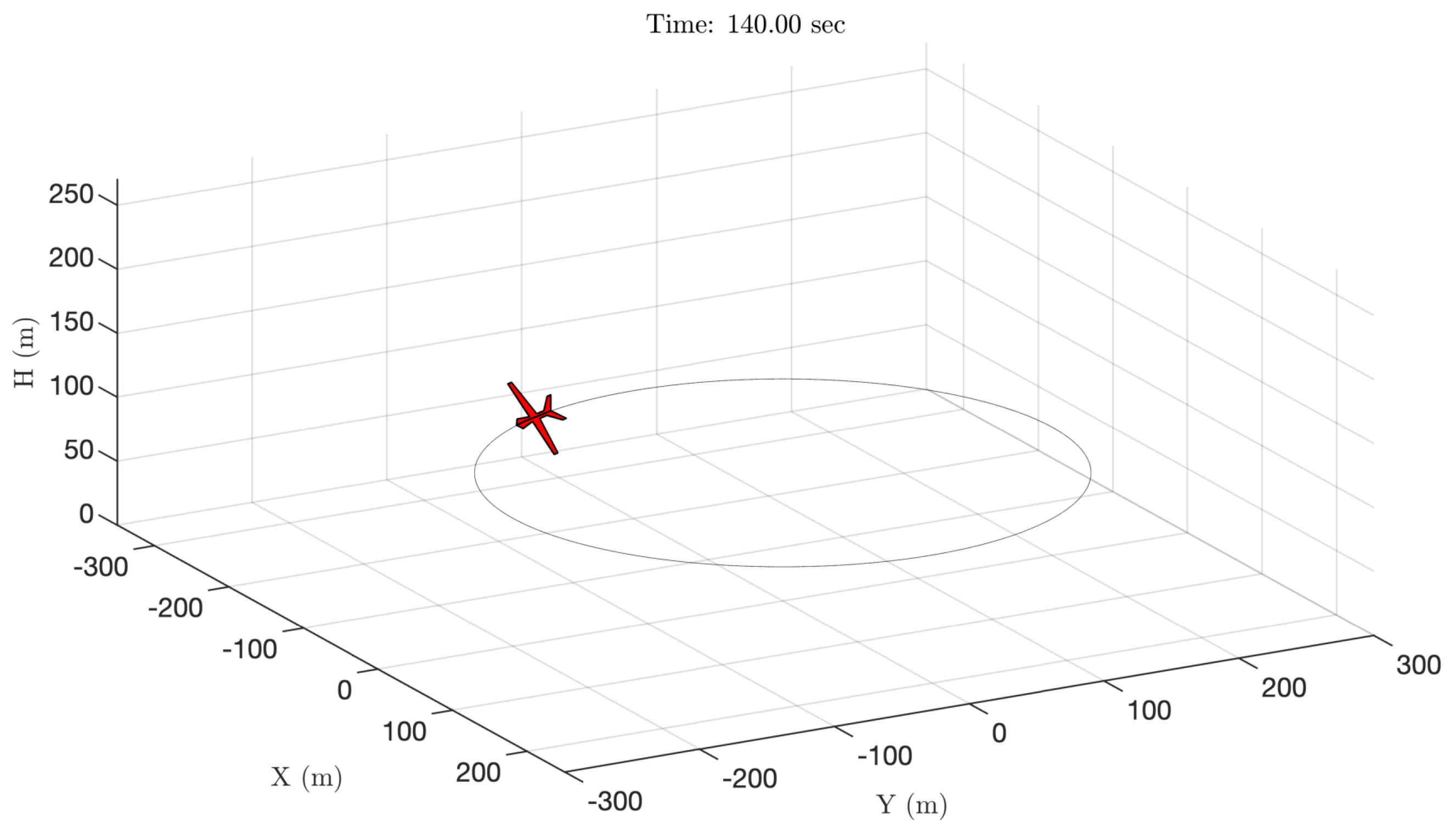
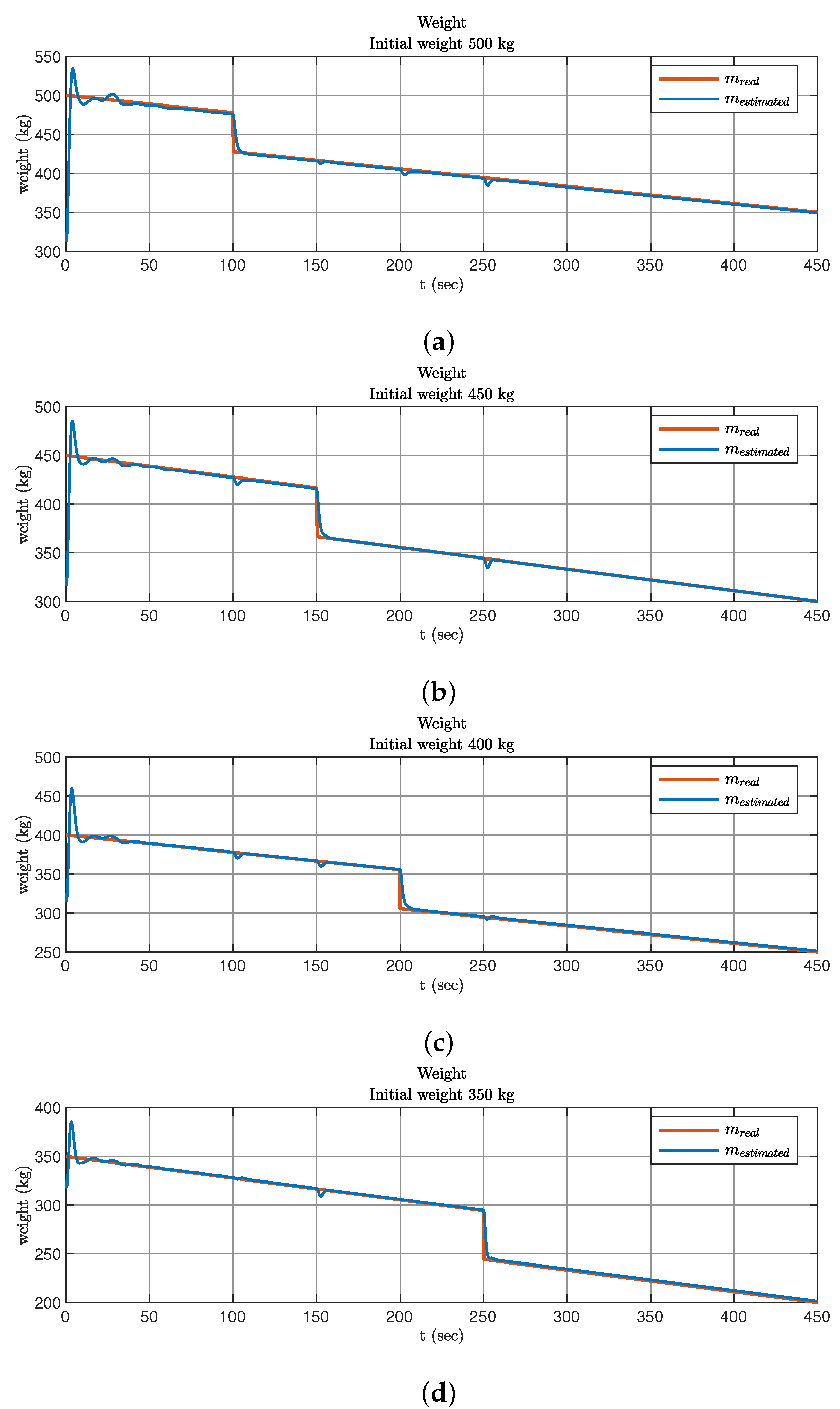
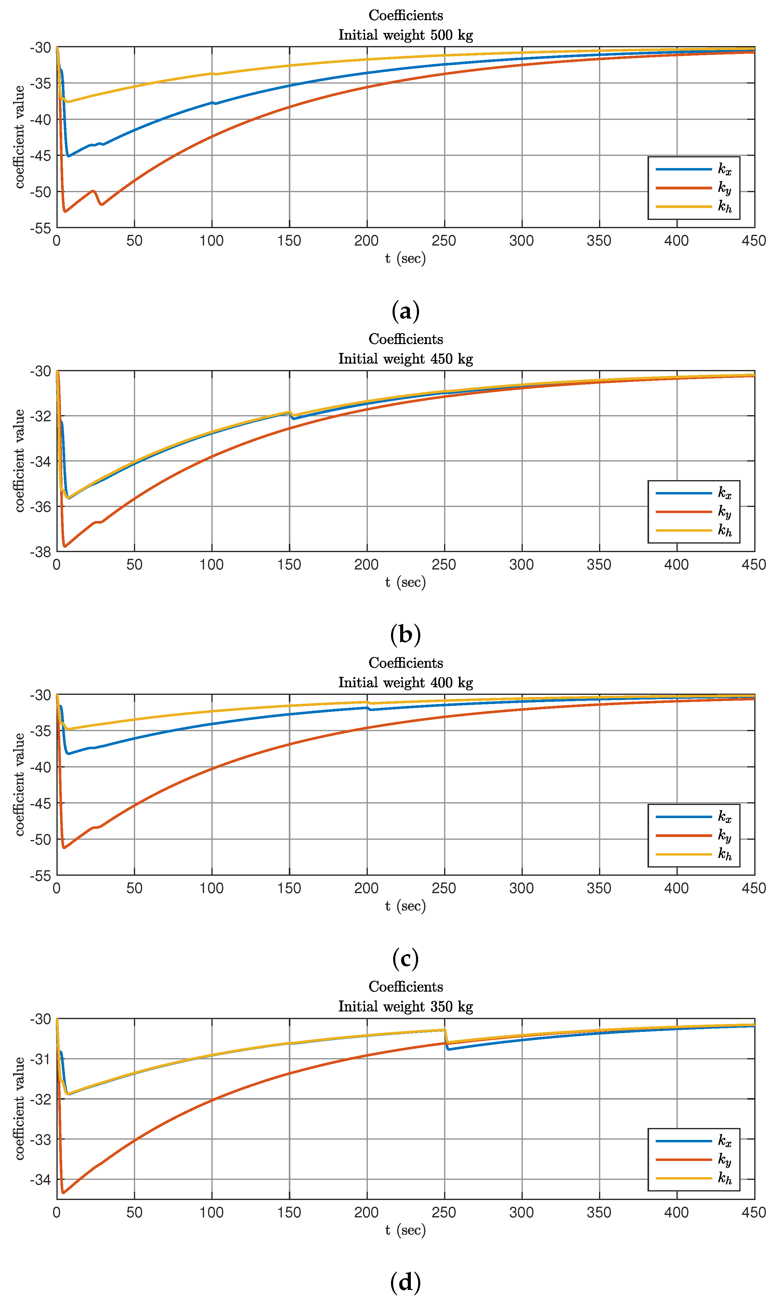
5.2.1. Control of Single UAV with Linearly Varying Mass

For the simulations, the UAV mass was considered in the form of a linear function in time with an initial value $m=400$ kg and slope $-0.4$ kg/s.

The simulation results are shown in Figure 4.

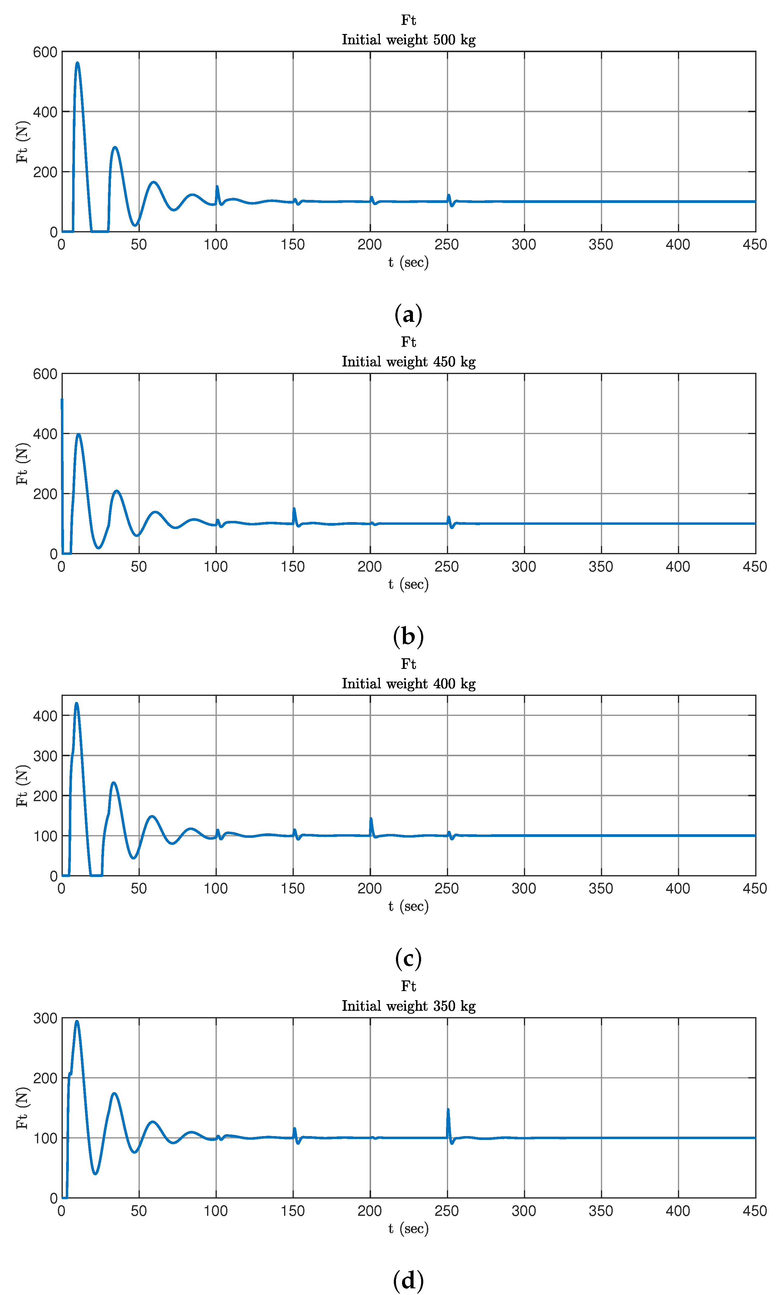
5.2.2. Control of Single UAV with Jump-changing Mass

Unknown UAV mass changes linearly until $t=200$ s; its initial value is 400 kg, and the slope is $-0.2$ kg/s. At time instant $t=200$ s, jumplike mass decreases 50 kg.

The simulation results are shown in Figure 5.

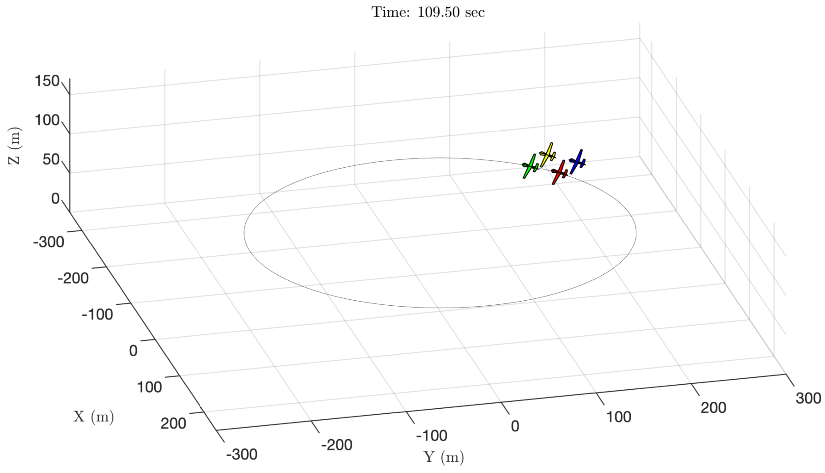
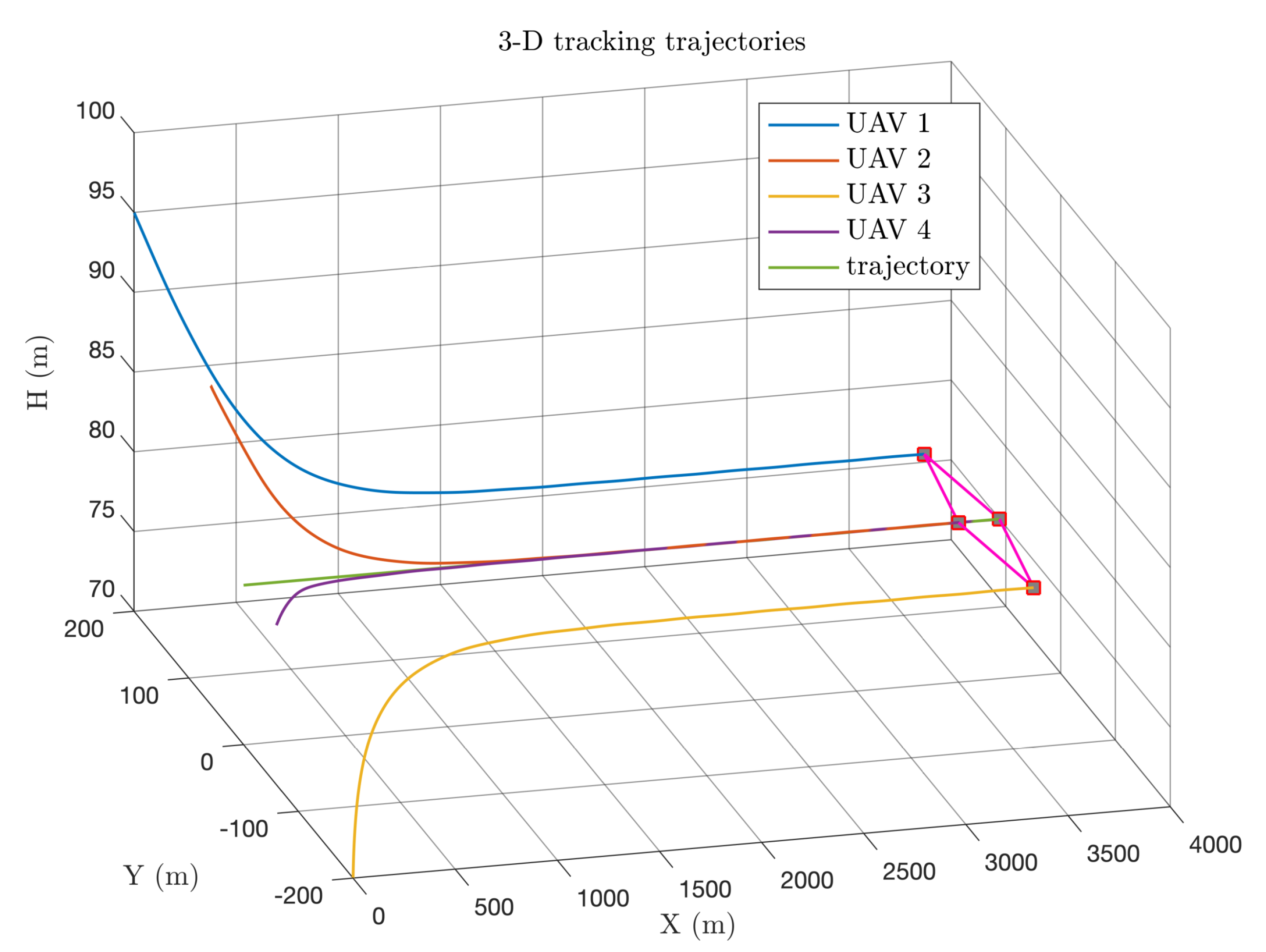
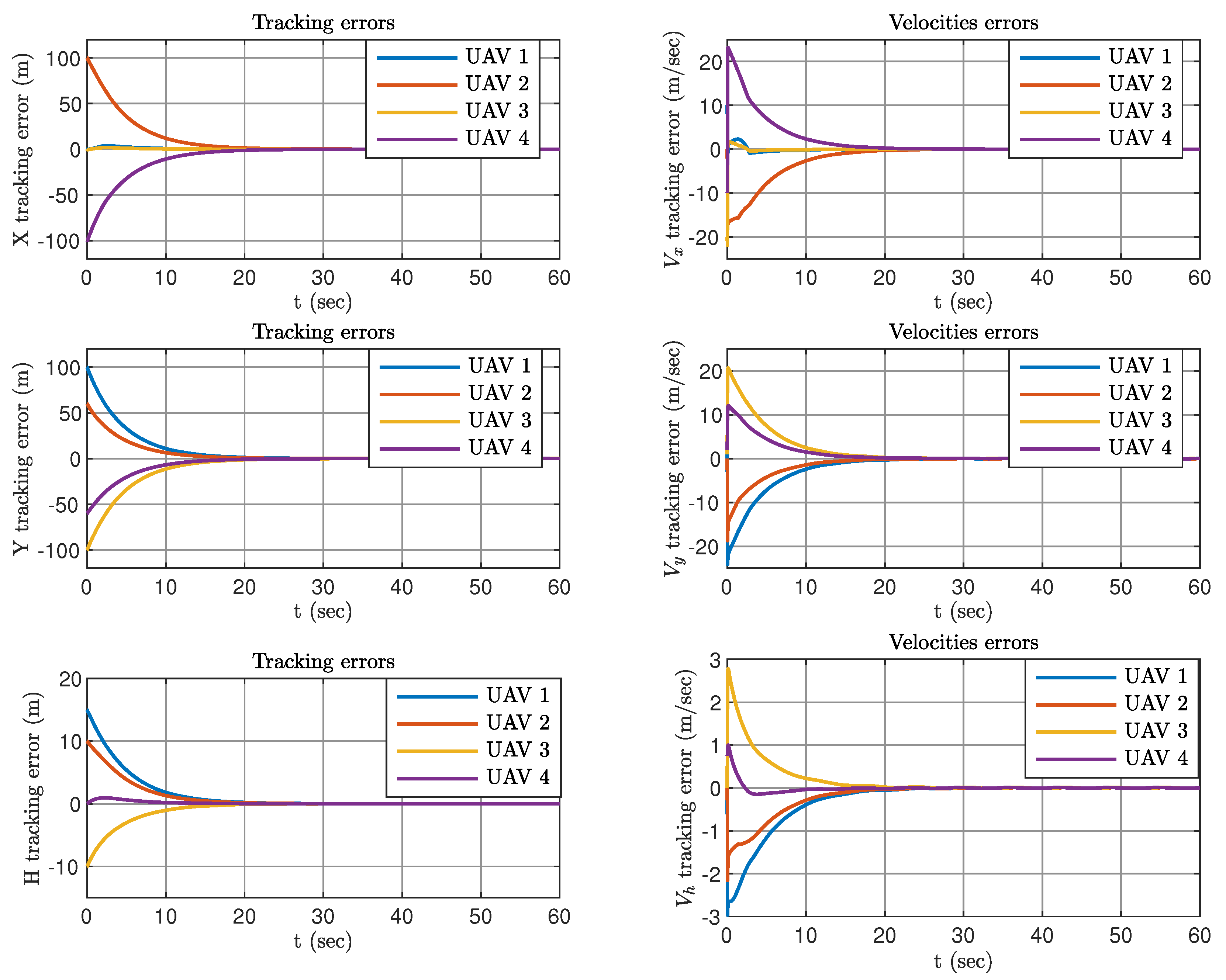
5.3. UAV Group Control

Next, we consider the control problem for a group of four autonomous UAVs. The formation is configured by offsets (49) and (50) relative to the reference trajectory (70):

$$\begin{array}{c}\hfill {\delta }_x={[0,-25,-25,-50]}^{\mathrm{T}},{\delta }_y={[0,25,-25,0]}^{\mathrm{T}},{\delta }_h={[0,0,0,0]}^{\mathrm{T}}.\end{array}$$

(71)

The consensus algorithm in form (62) was used to implement the group control. Data exchange between agents was carried out according to the connections graph shown in Figure 1.

The consensus algorithm parameters are as follows: $k_{xc}=k_{yc}=k_{hc}=350$, ${\rho }_x={\rho }_y={\rho }_h=250$.

The following common initial conditions for all UAVs of the group were used: initial speed $V_g\left(0\right)=50$ m/s; initial attitudes $\gamma \left(0\right)=0$ rad, $\psi \left(0\right)=\pi /2$ rad.

For the first UAV, the initial uncertain mass was $m=500$ kg, and the coordinates were $x\left(0\right)=50$ m, $y\left(0\right)=0$ m, $h\left(0\right)=75$ m. For the second UAV, the initial parameters were $m=450$ kg and the initial coordinates $x\left(0\right)=100$ m, $y\left(0\right)=30$ m, $h\left(0\right)=75$ m. For the third UAV, the initial uncertain mass was taken as $m=400$ kg and the initial coordinates $x\left(0\right)=0$ m, $y\left(0\right)=0$ m, $h\left(0\right)=75$ m. For the fourth UAV, the initial uncertain mass was taken as $m=350$ kg and the initial coordinates $x\left(0\right)=75$ m, $y\left(0\right)=0$ m, $h\left(0\right)=75$ m.

The masses of the agents change linearly with the same slope of $-0.22$ kg/s; in addition, each UAV loses 50 kg of mass once at time instants 100 s, 150 s, 200 s, and 250 s.

The simulation results are shown in Figure 6, Figure 7, Figure 8 and Figure 9. Figure 6 shows the errors in coordinates for each UAV in the group, Figure 7 demonstrates the mass estimates, Figure 8 shows the controller gains time histories, and Figure 9 shows the thrust forces time histories.

5.4. UAV Group Control under External Disturbances

To test the robustness properties of the obtained algorithms and compare them with other algorithms that solve similar problems, the results by Zhi et al. [26] for a four-agent formation were simulated. Control laws for group control (61) and (62) and tuning algorithms (69) were used.

The desired trajectory was

$$\begin{array}{c}\hfill r_x\left(t\right)=60t\mathrm{m},r_y\left(t\right),\equiv 0,r_h\left(t\right)=80\mathrm{m}.\end{array}$$

(72)

The following nominal parameters of the UAV were used: mass $m=20$ kg; wing area $S=1.37$ m${}^2$; air density ${\rho }_a=1.225$ kg/m${}^3$; zero-lift drag coefficient $C_{D_0}=0.02$; induced drag factor $k_c=0.1$. In the simulation, at the 25-th second of the flight the coefficients $C_{D_0}$ and $k_c=0.15$ increased abruptly by 50% (up to $C_{D_0}=0.03$, $k_c=0.15$).

The formation was configured by offsets (49) and (50) relative to the reference trajectory (72)

$$\begin{array}{c}\hfill {\delta }_x={[0,-100,0,100]}^{\mathrm{T}},{\delta }_y={[100,0,-100,0]}^{\mathrm{T}},{\delta }_h={[0,0,0,0]}^{\mathrm{T}}.\end{array}$$

(73)

The control laws (52), (61), (62) and tuning algorithm (69) parameters were identical for all the UAVs in the formation. In (52), the following output parameters $y_{xi}$, $y_{yi}$, $y_{hi}$ were used: ${\alpha }_{xi}={\alpha }_{yi}={\alpha }_{hi}=0.2182$. The constant parameters of control law (61) were set to $k_{xi}=k_{yi}=k_{hi}=0.4583$. The following adaptation algorithm (47) parameters were used: ${\gamma }_{mi}=15.5$, ${\sigma }_{mi}=0.008$, ${\gamma }_{xi}={\gamma }_{yi}={\gamma }_{hi}=15.5$, ${\sigma }_{xi}={\sigma }_{yi}={\sigma }_{hi}=0.008$, and the initial values of adjustable parameters were set to $m_{0i}=20$ kg, ${\widehat{k}}_{x0i}={\widehat{k}}_{y0i}={\widehat{k}}_{h0i}=-100$.

The consensus algorithm in form (62) was used to implement the group control. Data exchange between agents was carried out according to the connections graph shown in Figure 1. The consensus algorithm parameters were as follows: $k_{xc}=k_{yc}=k_{hc}=850$, ${\rho }_x={\rho }_y={\rho }_h=700$. The initial parameters were the same as in Zhi et al. [26].

The following common initial conditions were used for all UAVs in the group: initial attitudes $\gamma \left(0\right)=0$ rad, $\psi \left(0\right)=0$ rad.

For the first UAV, the initial uncertain mass was $m=24$ kg with initial coordinates $x\left(0\right)=0$ m, $y\left(0\right)=200$ m, $h\left(0\right)=95$ m, speed $V_g\left(0\right)=70$ m/s. For the second UAV, the initial uncertain mass was $m=17$ kg with initial coordinates $x\left(0\right)=0$ m, $y\left(0\right)=60$ m, $h\left(0\right)=90$ m, speed $V_g\left(0\right)=60$ m/s. For the third UAV, the initial uncertain mass was $m=22$ kg with initial coordinates $x\left(0\right)=0$ m, $y\left(0\right)=-200$ m, $h\left(0\right)=70$ m, speed $V_g\left(0\right)=40$ m/s. For the fourth UAV, the initial uncertain mass was $m=22$ kg with initial coordinates $x\left(0\right)=0$ m, $y\left(0\right)=-60$ m, $h\left(0\right)=80$ m, speed $V_g\left(0\right)=50$ m/s.

In addition, in the simulations the masses of agents changed linearly with the identical slope of $-0.083$ kg/s.

External perturbations $d_x$, $d_y$, $d_h$ were added to the first three equations of (1). The external disturbances were the same as in Zhi et al. [26], namely, $d_{x1}=0.5cos\left(t\right),$ $d_{y1}=0.8sin\left(t\right),$ $d_{h1}=0.5cos\left(t\right),$ $d_{x2}=4sin\left(t\right),$ $d_{y2}=3sin\left(t\right),$ $d_{h2}=4sin\left(t\right),$ $d_{x3}=\cos \left(2t\right),$ $d_{y3}=2sin\left(t\right),$ $d_{h3}=cos\left(2t\right),$ $d_{x4}=2cos\left(t\right),$ $d_{y4}=sin\left(t\right),$ $d_{h4}=2cos\left(t\right)$.

The simulation results are shown in Figure 10, Figure 11 and Figure 12. Figure 10 shows the 3D tracking trajectories, Figure 11 shows the tracking error comparison curves of three positions and three velocities, and Figure 12 shows the mass estimates.

Comparison of these results with those obtained by Zhi et al. [26] allows us to conclude that the algorithms presented in our paper show results no worse than in [26], while at the same time having a much simpler structure and lower number of adjustable parameters.

6. Discussion

At present, a great deal of work is being devoted to the UAV formation control problem. A detailed explanation of the differences between the present work and others is provided in

Table 1. Comparison with other works.

#	Other Works	This Work
1	[5] – tracking the moving ground target in the real-time; method: fuzzy-logic model-reference adaptive control (FL MRAC)	– tracking the given reference trajectory; method: implicit reference model (IRM) adaptive control
2	[20] – UAV parameters are known; method: non-adaptive control	– uncertain parameters: m, $C_{D_0}$, $k_c$, S; method: IRM adaptive control
3	[27] – UAV type: VTOL; control vector: command forces and torques; UAV parameters are known; method: adaptive estimation of disturbance	– UAV type: fixed-wing aircraft; control vector: $u={[F_{\mathrm{thrust}},C_L,\phi ]}^{\mathrm{T}}$; uncertain parameters: m, $C_{D_0}$, $k_c$, S; method: adaptive control with the IRM
4	[26] – control vector: $u={[F_{\mathrm{thrust}},n_{\mathrm{lf}},\phi ]}^{\mathrm{T}}$; uncertain parameters: $C_{D_0}$, $k_c$, S; method: robust adaptive controller	– control vector: $u={[F_{\mathrm{thrust}},C_L,\phi ]}^{\mathrm{T}}$; uncertain parameters: $m\left(t\right)$, $C_{D_0}$, $k_c$, S; method: adaptive control with the IRM
5	[28,31,32] – the reference trajectory is known only to the leading UAV; no consensus is ensured; UAV type: rotating-wing (quadrotor)	– each UAV has an information about the desired trajectory; consensus is ensured; UAV type: fixed-wing aircraft
6	[41] – single UAV; regulation of $V_g$, $\gamma$, tracking ${\psi }^{\ast }\left(t\right)$; point-mass dynamics model without kinematic relations; control vector: $u={[F_{\mathrm{thrust}},n_{\mathrm{lf}},\phi ]}^{\mathrm{T}}$; uncertain parameters: $C_{D_0},k_c$; method: adaptive control for non-affine plants	– group of UAVs; tracking the given reference trajectory; kinematic relations are included; control vector: $u={[F_{\mathrm{thrust}},C_L,\phi ]}^{\mathrm{T}}$; uncertain parameters: $m\left(t\right)$, $C_{D_0}$, $k_c$, S; method: IRM adaptive control
7	[42] – mission: passing a waypoint by several UAVs; control vector: $u={[F_{\mathrm{thrust}},n_{\mathrm{lf}},\phi ]}^{\mathrm{T}}$; parameters are known; method: optimal design of the behavioral approach of decentralized control; communication graph: undirected (ring topology)	– mission: tracking the given reference trajectory; control vector: $u={[F_{\mathrm{thrust}},C_L,\phi ]}^{\mathrm{T}}$; uncertain parameters: $m\left(t\right)$, $C_{D_0}$, $k_c$, S; method: IRM adaptive control; communication graph: directed
8	[43] – tracking the desired trajectory on the plane $(x_d\left(t\right),y_d\left(t\right))$; model: kinematic on the plane at constant height; control vector: $u={[V_g,\phi ]}^{\mathrm{T}}$; parameters: estimated by the Gaussian Process Regression training procedure; – communication graph: undirected	– tracking the desired trajectory in 3-D space; model: 3-D nonlinear point model; control vector: $u={[F_{\mathrm{thrust}},C_L,\phi ]}^{\mathrm{T}}$; uncertain parameters: $m\left(t\right)$, $C_{D_0}$, $k_c$, S; communication graph: directed

. Each row (item) of the table contains the distinctive features of this paper as compared to those noted in the corresponding item; for brevity and clarity, similar properties are not indicated. The following characteristics are notable: generation of the desired trajectory (whether it is predefined or generated depending on the current situation); type of UAV; control/adaptation method; set of uncertain UAV parameters; control vector components; whether or not consensus is ensured; model of UAV motion; and communication graph topology.

7. Conclusions

In this paper, we have proposed a new feedback-linearized UAV model with point mass. A linear model with an unknown value of the UAV mass was obtained via transformation. The velocity gradient method was applied to obtain a combined adaptive control law that includes equations for estimating the unknown mass value and for tuning the parameters of a linear controller with an implicit reference model. The obtained new adaptive algorithms were used to solve the problem of decentralized control of a UAV formation with an unknown mass based on a consensus algorithm. Rigorous stability conditions for control and identification are presented. Computer simulations of the obtained algorithms for both a single UAV and a UAV formation show good performance of the proposed approach under conditions of variable UAV mass. Further research might involve considering the influence of wind on the movement of the UAVs, as well as considering situations in which not every UAV has access to information about the movement trajectory.

References

1. Du, N.; Zhou, Y.; Deng, W.; Luo, Q. Improved chimp optimization algorithm for three-dimensional path planning problem. Multimed. Tools Appl. 2022, 81, 27397–27422. [Google Scholar] [CrossRef]
2. Sefati, S.; Halunga, S.; Farkhady, R. Cluster selection for load balancing in flying ad hoc networks using an optimal low-energy adaptive clustering hierarchy based on optimization approach. Aircr. Eng. Aerosp. Technol. 2022, 94, 1344–1356. [Google Scholar] [CrossRef]
3. Trujillo, M.; Becerra, H.; Gómez-Gutiérrez, D.; Ruiz-León, J.; Ramírez-Treviño, A. Hierarchical task-based formation control and collision avoidance of UAVs in finite time. Eur. J. Control 2021, 60, 48–64. [Google Scholar] [CrossRef]
4. Luo, L.; Wang, X.; Ma, J.; Ong, Y. GrpAvoid: Multigroup Collision-Avoidance Control and Optimization for UAV Swarm. IEEE Trans. Cybern. 2021. [Google Scholar] [CrossRef] [PubMed]
5. Muslimov, T.; Munasypov, R. Multi-UAV cooperative target tracking via consensus-based guidance vector fields and fuzzy MRAC. Aircr. Eng. Aerosp. Technol. 2021, 93, 1204–1212. [Google Scholar] [CrossRef]
6. Asami, K.; Bai, Y.; Svinin, M.; Hatayama, M. Survivor searching in a dynamically changing flood zone by multiple unmanned aerial vehicles. Artif. Life Robot. 2022, 27, 292–299. [Google Scholar] [CrossRef]
7. Islam, S.; DIas, J.; Sunda-Meya, A. Distributed Tracking Synchronization Protocol for a Networked of Leader-follower Unmanned Aerial Vehicles with Uncertainty. In Proceedings of the Industrial Electronics Conference (IECON 2021), Toronto, Canada, 13–16 October 2021. [Google Scholar] [CrossRef]
8. Cucker, F.; Smale, S. Emergent Behavior in Flocks. IEEE Trans. Autom. Control 2007, 52, 852–862. [Google Scholar] [CrossRef] [Green Version]
9. Song, Y.; Gu, M.; Choi, J.; Oh, H.; Lim, S.; Shin, H.S.; Tsourdos, A. Using Lazy Agents to Improve the Flocking Efficiency of Multiple UAVs. J. Intell. Robot. Syst. Theory Appl. 2021, 103. [Google Scholar] [CrossRef]
10. Zhou, P.; Chen, B. Semi-global leader-following consensus-based formation flight of unmanned aerial vehicles. Chin. J. Aeronaut. 2022, 35, 31–43. [Google Scholar] [CrossRef]
11. Ahmed, A.; Naeem, M.; Al-Dweik, A. Joint Optimization of Sensors Association and UAVs Placement in IoT Applications With Practical Network Constraints. IEEE Access 2021, 9, 7674–7689. [Google Scholar] [CrossRef]
12. Chen, L.; Zhao, R.; He, K.; Zhao, Z.; Fan, L. Intelligent ubiquitous computing for future UAV-enabled MEC network systems. Clust. Comput. 2022, 25, 2417–2427. [Google Scholar] [CrossRef]
13. Mahmood, A.; Vu, T.; Khan, W.U.; Chatzinotas, S.; Ottersten, B. Optimizing Computational and Communication Resources for MEC Network Empowered UAV-RIS Communication. Preprint 2022. [Google Scholar] [CrossRef]
14. Lin, Z.; Lin, M.; Wang, J.B.; de Cola, T.; Wang, J. Joint Beamforming and Power Allocation for Satellite-Terrestrial Integrated Networks With Non-Orthogonal Multiple Access. IEEE J. Sel. Top. Signal Process. 2019, 13, 657–670. [Google Scholar] [CrossRef] [Green Version]
15. Güzey, H.; Güzey, N. Adaptive hybrid formation-search and track controller of UAVs. Int. J. Syst. Sci. 2022, 53, 2301–2317. [Google Scholar] [CrossRef]
16. Mahfouz, M.; Hafez, A.; Ashry, M.; Elnashar, G. Target Assignment for Cooperative Quadrotors Unmanned Aerial Vehicles. J. Phys. Conf. Ser. 2021, 2128. [Google Scholar] [CrossRef]
17. Han, Q.; Zhou, Y.; Liu, X.; Tuo, X. Event-Triggered Finite-Time Attitude Cooperative Control for Multiple Unmanned Aerial Vehicles. Appl. Bionics Biomech. 2022, 2022, 5875004. [Google Scholar] [CrossRef]
18. Wu, X.; Wu, Y.; Xu, Z.; Chen, Q. Fixed-time flocking formation of nonlinear multi-agent system with uncertain state perturbation. Int. J. Control. 2022. [Google Scholar] [CrossRef]
19. Gong, J.; Jiang, B.; Ma, Y.; Mao, Z. Distributed Adaptive Fault-Tolerant Formation Control for Heterogeneous Multiagent Systems With Communication Link Faults. IEEE Trans. Aerosp. Electron. Syst. 2022, 1–11. [Google Scholar] [CrossRef]
20. Popov, A.M.; Kostin, I.; Fadeeva, J.; Andrievsky, B. Development and Simulation of Motion Control System for Small Satellites Formation. Electronics 2021, 10, 3111. [Google Scholar] [CrossRef]
21. Popov, A.M.; Kostrygin, D.G.; Krashanin, P.V.; Shevchik, A.A. Development of Algorithm for Guiding the Swarm of Unmanned Aerial Vehicles. In Proceedings of the 29th Saint Petersburg International Conference on Integrated Navigation Systems (ICINS 2022), Saint Petersburg, Russia, 30 May–1 June 2022; Volume 1, pp. 1–4. [Google Scholar] [CrossRef]
22. Gamagedara, K.; Lee, T. Geometric Adaptive Controls of a Quadrotor Unmanned Aerial Vehicle with Decoupled Attitude Dynamics. J. Dyn. Syst. Meas. Control. ASME 2022, 144, 031002. [Google Scholar] [CrossRef]
23. Chatterjee, B.; Dutta, R. Studying the Effect of Network Latency on an Adaptive Coordinated Path Planning Algorithm for UAV Platoons. In Proceedings of the 2022 8th Workshop on Micro Aerial Vehicle Networks, Systems, and Applications (DroNet 2022), Part of MobiSys 2022, Portland, OR, USA, 27 June–1 July 2022; pp. 7–12. [Google Scholar] [CrossRef]
24. Ullah, N.; Mehmood, Y.; Aslam, J.; Wang, S.; Phoungthong, K. Fractional order adaptive robust formation control of multiple quad-rotor UAVs with parametric uncertainties and wind disturbances. Chin. J. Aeronaut. 2022, 35, 204–220. [Google Scholar] [CrossRef]
25. Liang, W.; Chen, Z.; Yao, B. Geometric Adaptive Robust Hierarchical Control for Quadrotors With Aerodynamic Damping and Complete Inertia Compensation. IEEE Trans. Ind. Electron. 2022, 69, 13213–13224. [Google Scholar] [CrossRef]
26. Zhi, Y.; Liu, L.; Guan, B.; Wang, B.; Cheng, Z.; Fan, H. Distributed robust adaptive formation control of fixed-wing UAVs with unknown uncertainties and disturbances. Aerosp. Sci. Technol. 2022, 126, 107600. [Google Scholar] [CrossRef]
27. Huang, Y.; Meng, Z. Bearing-Based Distributed Formation Control of Multiple Vertical Take-Off and Landing UAVs. IEEE Trans. Control Netw. Syst. 2021, 8, 1281–1292. [Google Scholar] [CrossRef]
28. Andrievsky, B.; Tomashevich, S. Passification based signal-parametric adaptive controller for agents in formation. IFAC-PapersOnLine 2015, 48, 222–226. [Google Scholar] [CrossRef]
29. Andrievskii, B.; Fradkov, A. Method of passification in adaptive control, estimation, and synchronization. Autom. Remote Control 2006, 67, 1699–1731. [Google Scholar] [CrossRef]
30. Andrievskii, B.R.; Selivanov, A.A. New Results on the Application of the Passification Method. A Survey. Automat. Remote Control 2018, 79, 957–995. [Google Scholar] [CrossRef]
31. Tomashevich, S.; Andrievsky, B. Adaptive control of quadrotors spatial motion in formation with implicit reference model. AIP Conf. Proc. 2018, 2046, 020103. [Google Scholar] [CrossRef]
32. Tomashevich, S.; Andrievsky, B. High-order adaptive control in multi-agent quadrotor formation. Math. Eng. Sci. Aerosp. 2019, 10, 681–693. [Google Scholar]
33. Furtat, I.B. Simple Adaptive Algorithm for Plants with Input Delay and Disturbances. IFAC-PapersOnLine 2017, 50, 4270–4275. [Google Scholar] [CrossRef]
34. Tomashevich, S.I. Control for a system of linear agents based on a high order adaptation algorithm. Autom. Remote Control 2017, 78, 276–288. [Google Scholar] [CrossRef]
35. Tomashevich, S.; Belyavskyi, A. 2DoF indoor testbed for quadrotor identification and control. In Proceedings of the 23rd Saint Petersburg International Conference Integrated Navigation Systems (ICINS 2016), Saint Petersburg, Russia, 30 May–1 June 2016; pp. 373–376. [Google Scholar]
36. Andrievsky, B.; Popov, A.M.; Kostin, I.; Fadeeva, J. Modeling and Control of Satellite Formations: A Survey. Automation 2022, 3, 511–544. [Google Scholar] [CrossRef]
37. Andrievsky, B.; Fradkov, A.; Kudryashova, E. Control of two satellites relative motion over the packet erasure communication channel with limited transmission rate based on adaptive coder. Electronics 2020, 9, 2032. [Google Scholar] [CrossRef]
38. Kuznetsov, N.V.; Andrievsky, B.; Kudryashova, E.V.; Kuznetsova, O.A. Stability and hidden oscillations analysis of the spacecraft attitude control system using reaction wheels. Aerosp. Sci. Technol. 2022, 131, 107973. [Google Scholar] [CrossRef]
39. Menon, P.K.A. Short-range nonlinear feedback strategies for aircraft pursuit-evasion. J. Guid. Control. Dyn. 1989, 12, 27–32. [Google Scholar] [CrossRef]
40. Menon, P.K.; Sweriduk, G.D.; Sridhar, B. Optimal Strategies for Free-Flight Air Traffic Conflict Resolution. J. Guid. Control. Dyn. 1999, 22, 202–211. [Google Scholar] [CrossRef] [Green Version]
41. Boskovic, J.D.; Chen, L.; Mehra, R.K. Adaptive Control Design for Nonaffine Models Arising in Flight Control. J. Guid. Control. Dyn. 2004, 27, 209–217. [Google Scholar] [CrossRef]
42. Kim, S.; Kim, Y. Optimum design of three-dimensional behavioural decentralized controller for UAV formation flight. Eng. Optim. 2009, 41, 199–224. [Google Scholar] [CrossRef]
43. Wang, J.; Xin, M. Integrated Optimal Formation Control of Multiple Unmanned Aerial Vehicles. IEEE Trans. Control Syst. Technol. 2013, 21, 1731–1744. [Google Scholar] [CrossRef]
44. Beard, R.W.; McLain, T.W. Small Unmanned Aircraft: Theory and Practice; Princeton University Press: Princeton, NJ, USA, 2012. [Google Scholar]
45. Dobrokhodov, V. Kinematics and Dynamics of Fixed-Wing UAVs. In Handbook of Unmanned Aerial Vehicles; Springer Netherlands: Dordrecht, The Netherlands, 2015; pp. 243–277. [Google Scholar] [CrossRef]
46. Miele, A. Flight Mechanics: Theory of Flight Paths; Dover Publications Inc.: New York, NY, USA, 2016. [Google Scholar]
47. Zhao, Y.; Tsiotras, P. Time-Optimal Path Following for Fixed-Wing Aircraft. J. Guid. Control. Dyn. 2013, 36, 83–95. [Google Scholar] [CrossRef] [Green Version]
48. Anderson, M.; Robbins, A. Formation flight as a cooperative game. In Proceedings of the Guidance, Navigation, and Control Conference and Exhibit; AIAA: Boston, MA, USA, 1998; p. 244. [Google Scholar] [CrossRef]
49. Khalil, H.K. Nonlinear Systems, 3rd ed.; Prentice-Hall: Upper Saddle River, NJ, USA, 2002. [Google Scholar]
50. Fliess, M.; Lévine, J.; Martin, P.; Rouchon, P. Flatness and defect of non-linear systems: Introductory theory and examples. Int. J. Control 1995, 61, 1327–1361. [Google Scholar] [CrossRef] [Green Version]
51. Lévine, J. Analysis and Control of Nonlinear Systems A Flatness-Based Approach; Springer: Berlin/Heidelberg, Germany, 2009. [Google Scholar] [CrossRef]
52. Fradkov, A.L. Speed-gradient scheme and its application in adaptive control problems. Autom. Remote Control 1980, 40, 1333–1342. [Google Scholar]
53. Fradkov, A.L.; Miroshnik, I.V.; Nikiforov, V.O. Nonlinear and Adaptive Control of Complex Systems; Kluwer: Dordrecht, The Netherlands, 1999. [Google Scholar]
54. Andrievsky, B.R.; Fradkov, A.L. Speed Gradient Method and Its Applications. Autom. Remote Control 2021, 82, 1463–1518. [Google Scholar] [CrossRef]
55. Fradkov, A.L.; Andrievsky, B. Speed-Gradient Method in Mechanical Engineering. Adv. Struct. Mater. 2022, 164, 171–194. [Google Scholar] [CrossRef]
56. Fradkov, A.L. Synthesis of an adaptive system for linear plant stabilization. Autom. Remote Control 1974, 35, 1960–1966. [Google Scholar]
57. Fradkov, A. Lyapunov-Bregman functions for speed-gradient adaptive control of nonlinear time-varying systems. IFAC-PapersOnLine 2022, 55, 544–548. [Google Scholar] [CrossRef]
58. Fradkov, A.; Andrievsky, B. Adaptive Synchronization of Time-Varying Non-linear Systems with Application to Signal Transmission. Stud. Syst. Decis. Control 2022, 414, 325–344. [Google Scholar] [CrossRef]
59. Fradkov, A.; Tomashevich, S.; Andrievsky, B.; Amelin, K.; Kaliteevskiy, I. Adaptive Coding For Data Exchange Between Quadrotors In The Formation. IFAC-PapersOnLine 2016, 49, 275–280. [Google Scholar] [CrossRef]
60. Marantos, P.; Koveos, Y.; Kyriakopoulos, K. UAV State Estimation Using Adaptive Complementary Filters. IEEE Trans. Control Syst. Technol. 2016, 24, 1214–1226. [Google Scholar] [CrossRef]
61. Yu, Y.; Peng, S.; Li, Q.; Dong, X.; Ren, Z. Cooperative Navigation Method Based on Adaptive CKF for UAVs in GPS Denied Areas. In Proceedings of the IEEE CSAA Guidance, Navigation and Control Conference, CGNCC 2018, Xiamen, China, 10–12 August 2018. [Google Scholar] [CrossRef]
62. Silantyev, A.; Tereshchenko, D.; Kazakov, L.; Selyanskaya, E. Adaptive system of mutual positioning for controlling the groups of unmanned aerial vehicles. In Proceedings of the 2018 Systems of Signal Synchronization, Generating and Processing in Telecommunications (SYNCHROINFO 2018), Minsk, Belarus, 4–5 July 2018. [Google Scholar] [CrossRef]
63. Tomashevich, S.; Andrievsky, B.; Fradkov, A. Formation control of a group of unmanned aerial vehicles with data exchange over a packet erasure channel. In Proceedings of the 2018 IEEE Industrial Cyber-Physical Systems (ICPS 2018), Saint Petersburg, Russia, 15–18 May 2018; pp. 38–43. [Google Scholar] [CrossRef]
64. Zhong, W.; Xu, L.; Liu, X.; Zhu, Q.; Zhou, J. Adaptive beam design for UAV network with uniform plane array. Phys. Commun. 2019, 34, 58–65. [Google Scholar] [CrossRef]
65. Darabkh, K.; Alfawares, M.; Althunibat, S. MDRMA: Multi-data rate mobility-aware AODV-based protocol for flying ad-hoc networks. Veh. Commun. 2019, 18. [Google Scholar] [CrossRef]
66. Tomashevich, S.; Andrievsky, B.; Dokuchaeva, A.; Emelyanov, V. Navigation data exchange between UAVs in the formation by means of the adaptive coding procedure. Math. Eng. Sci. Aerosp. 2019, 10, 463–478. [Google Scholar]
67. Amelin, K.; Andrievsky, B.; Tomashevich, S.; Fradkov, A. Data Exchange with Adaptive Coding between Quadrotors in a Formation. Autom. Remote Control 2019, 80, 150–163. [Google Scholar] [CrossRef]
68. Lim, S.; Song, Y.; Choi, J.; Myung, H.; Lim, H.; Oh, H. Decentralized Hybrid Flocking Guidance for a Swarm of Small UAVs. In Proceedings of the 2019 International Workshop on Research, Education and Development on Unmanned Aerial Systems, RED-UAS 2019, Cranfield, UK, 25–27 November 2019; pp. 287–296. [Google Scholar] [CrossRef]
69. Lin, Z.; An, K.; Niu, H.; Hu, Y.; Chatzinotas, S.; Zheng, G.; Wang, J. SLNR-based Secure Energy Efficient Beamforming in Multibeam Satellite Systems. IEEE Trans. Aerosp. Electron. Syst. 2022, 1–4. [Google Scholar] [CrossRef]
70. Lin, Z.; Lin, M.; de Cola, T.; Wang, J.B.; Zhu, W.P.; Cheng, J. Supporting IoT With Rate-Splitting Multiple Access in Satellite and Aerial-Integrated Networks. IEEE Internet Things J. 2021, 8, 11123–11134. [Google Scholar] [CrossRef]
71. Lin, Z.; Niu, H.; An, K.; Wang, Y.; Zheng, G.; Chatzinotas, S.; Hu, Y. Refracting RIS-Aided Hybrid Satellite-Terrestrial Relay Networks: Joint Beamforming Design and Optimization. IEEE Trans. Aerosp. Electron. Syst. 2022, 58, 3717–3724. [Google Scholar] [CrossRef]
72. Geraci, G.; Garcia-Rodriguez, A.; Azari, M.M.; Lozano, A.; Mezzavilla, M.; Chatzinotas, S.; Chen, Y.; Rangan, S.; Renzo, M.D. What Will the Future of UAV Cellular Communications Be? A Flight From 5G to 6G. IEEE Commun. Surv. Tutorials 2022, 24, 1304–1335. [Google Scholar] [CrossRef]
73. Dovgal, V. Making decisions about the placement of unmanned aerial vehicles based on the implementation of an artificial immune system in relation to information processing. In Proceedings of the International Conference on Industrial Engineering, Applications and Manufacturing (ICIEAM 2021), Sochi, Russia, 17–21 May 2021; pp. 828–833. [Google Scholar] [CrossRef]
74. Wu, P.; Xiao, F.; Huang, H.; Sha, C.; Yu, S. Adaptive and Extensible Energy Supply Mechanism for UAVs-Aided Wireless-Powered Internet of Things. IEEE Internet Things J. 2020, 7, 9201–9213. [Google Scholar] [CrossRef]
75. Wei, X.; Yang, J.; Fan, X. Fully distributed guidance laws for unmanned aerial vehicles formation flight. Trans. Inst. Meas. Control 2020, 42, 965–980. [Google Scholar] [CrossRef]
76. Ren, W.; Beard, R.W. Distributed Consensus in Multi-Vehicle Cooperative Control; Springer: London, UK, 2008. [Google Scholar] [CrossRef]
77. Olfati-Saber, R.; Murray, R. Consensus problems in networks of agents with switching topology and time-delays. IEEE Trans. Autom. Control 2004, 49, 1520–1533. [Google Scholar] [CrossRef] [Green Version]
78. Olfati-Saber, R.; Fax, J.A.; Murray, R.M. Consensus and Cooperation in Networked Multi-Agent Systems. Proc. IEEE 2007, 95, 215–233. [Google Scholar] [CrossRef] [Green Version]
79. Kabiri, M.; Atrianfar, H.; Menhaj, M. Formation control of VTOL UAV vehicles under switching-directed interaction topologies with disturbance rejection. Int. J. Control 2018, 91, 33–44. [Google Scholar] [CrossRef]
Figure 1. Communication graph.
Electronics 11 04187 g001
Figure 2. UAV trajectory for adaptive control case.
Electronics 11 04187 g002
Figure 3. UAV trajectory for group control case.
Electronics 11 04187 g003
Figure 4. Coordinate errors (a), estimated mass value (b), controller gains (c), and thrust force (d) for a scenario in which the UAV mass changes linearly over time.
Electronics 11 04187 g004
Figure 5. Coordinate errors (a), estimated mass value (b), controller gains (c), and thrust force (d) for scenario of jumplike UAV mass changing.
Electronics 11 04187 g005
Figure 6. Coordinate errors for control the case of a group of UAVs of variable mass with initial mass values: 500 kg (a), 450 kg (b), 400 kg (c), 350 kg (d).
Electronics 11 04187 g006
Figure 7. Estimated mass values when controlling a group of UAVs of variable mass with initial mass values of 500 kg (a), 450 kg (b), 400 kg (c), and 350 kg (d).
Electronics 11 04187 g007
Figure 8. Coefficients of regulators when controlling a group of UAVs of variable mass with initial mass values of 500 kg (a), 450 kg (b), 400 kg (c), and 350 kg (d).
Electronics 11 04187 g008
Figure 9. Thrust forces for the case of a group of variable mass UAVs control with initial mass values of 500 kg (a), 450 kg (b), 400 kg (c), and 350 kg (d).
Electronics 11 04187 g009
Figure 10. 3D tracking trajectories.
Electronics 11 04187 g010
Figure 11. Tracking error comparison curves of three positions and three velocities.
Electronics 11 04187 g011
Figure 12. Estimated masses of UAVs in group.
Electronics 11 04187 g012