Learnable Wavelet Scattering Networks: Applications to Fault Diagnosis of Analog Circuits and Rotating Machinery

Abstract

Analog circuits are a critical part of industrial electronics and systems. Estimates in the literature show that, even though analog circuits comprise less than 20% of all circuits, they are responsible for more than 80% of faults. Hence, analog circuit fault diagnosis and isolation can be a valuable means of ensuring the reliability of circuits. This paper introduces a novel technique of learning time–frequency representations, using learnable wavelet scattering networks, for the fault diagnosis of circuits and rotating machinery. Wavelet scattering networks, which are fixed time–frequency representations based on existing wavelets, are modified to be learnable so that they can learn features that are optimal for fault diagnosis. The learnable wavelet scattering networks are developed using the genetic algorithm-based optimization of second-generation wavelet transform operators. The simulation and experimental results for the diagnosis of analog circuit faults demonstrates that the developed diagnosis scheme achieves greater fault diagnosis accuracy than other methods in the literature, even while considering a larger number of fault classes. The performance of the diagnosis scheme on benchmark datasets of bearing faults and gear faults shows that the developed method generalizes well to fault diagnosis in multiple domains and has good transfer learning performance, too.

1. Introduction

Electronic circuits are ubiquitous in our everyday lives, in applications ranging from the commercial domain to the safety-critical domain. As a result, unforeseen circuit failures can have enormous consequences for the safety and financial well-being of their users and producers [1,2]. Analog circuit failures can be attributed to interconnected failures or component faults, which are associated with either parametric drift (soft faults) or short circuit/open circuit [3] (hard faults). Analog circuits have become increasingly complex and consequentially, fault diagnosis is increasingly difficult, due to: (a) component tolerances, (b) interactions among components, (c) inadequate accessible measurement nodes; and (d) the inherent non-linearity in the behavior of analog circuits. Compared to digital circuits, analog circuits are more susceptible to interference and have fewer measurement nodes. Interestingly, even though analog circuits account for less than 20% of all circuits, they are responsible for more than 80% of circuit faults [4,5] Therefore, the fault diagnosis of analog circuits has become a highly important research area in recent years.

There are two broad categories for fault diagnosis approaches for circuits: analytical methods and data-driven methods. Circuit transfer function equations are required to apply analytical methods [6]. If these equations are unavailable, they can be determined using design principles or parameter identification techniques [7], and fault diagnosis is then achieved by exposing the circuit to a test stimulus and using the response to estimate the circuit parameters. This technique is suitable for linear analog circuits but is not feasible for nonlinear analog circuits because of the complexity involved [8].

Data-driven methods [9,10,11,12] require data obtained under faulty conditions to be available either through testing, operation, or simulation such that a comparison can be made to data obtained under healthy conditions for fault diagnosis. Features of the data are used for this comparison and can be time domain, frequency domain, or time–frequency domain. Various machine learning approaches such as neural networks, support vector machines, Naïve Bayes classifier, etc., have been used for fault diagnosis under the broad umbrella of data-driven methods. Neural-network-based fault-diagnosis approaches [13,14] have included, for feature generation: kurtosis and entropy [15], wavelet transforms [16], and fractional wavelet transforms [17]; and for dimensionality reduction: kernel PCA (kPCA) [16,17]. Support vector machine (SVM)-based [18] fault-diagnosis approaches have further included, for feature generation: fractional Fourier transform [19], cross-wavelet transform [20,21], deep belief networks (DBN) [22,23], and empirical mode decomposition [24]; for dimensionality reduction: parametric t-SNE [20] and principal component analysis [21]; and for SVM hyperparameter optimization: the double-chains quantum genetic algorithm [24], the fruitfly algorithm [25], the barnacles mating optimizer algorithm [26], and the firefly algorithm [27]. Naïve-Bayes-classifier-based [28] fault-diagnosis approaches include, for feature generation: cross-wavelet transform [29]; and for dimensionality reduction: bilateral 2D linear discriminant analysis.

The standard approach that the vast majority of the methods followed is to extract features and apply a dimensionality reduction algorithm to obtain a lower-dimensional feature set which is then fed to a classification algorithm. Extracting features informative for fault diagnosis requires technical expertise which restricts its application as a generalized method. Recently, techniques have been proposed involving the direct application of deep learning methods for fault diagnosis. These techniques use input data to learn features autonomously through a multi-layered neural network. This avoids the need for manual feature extraction and feature selection. For example, different 2D representations [30,31] have been developed for circuit outputs for use with state-of-the-art deep learning networks such as ResNet50 [32] to achieve fault diagnosis. However, the creation of an optimal custom deep learning network structure for the problem at hand requires subject matter expertise and extensive trial-and-error [33]. Inspired by wavelet scattering theory [34] and second-generation wavelet transform [35], we propose a novel technique that does not need to be optimized for structure and learns wavelet filters instead of random filters from the data. Hence, it overcomes the shortcomings of deep learning networks. The remainder of the paper is organized as follows: Section 2 presents a theoretical background of the techniques involved in the approach. Section 3 details the developed fault diagnosis methodology. Section 4 details the application of the approach to the fault diagnosis of two circuits and a bearing and a gears dataset. The conclusions follow in Section 5.

2. Theoretical Background

As mentioned earlier, in this paper, time–frequency representations are learnt from the circuit outputs for fault diagnosis using learnable wavelet scattering networks (LWSNs). This involves modifying wavelet scattering networks, which are fixed time–frequency representations based on existing wavelets, such that they can learn features that are optimal for fault diagnosis. Learnable wavelet scattering networks are developed using the genetic-algorithm-based optimization of second-generation wavelet transform operators. Support vector machines (SVMs) are used as classifiers for the features learned by the LWSN. In the following subsections, we review the basics of a wavelet transform, a wavelet scattering network, a genetic algorithm, and a support vector machine and introduce the concept of learnable wavelet scattering networks.

2.1. Wavelet Transform

A wavelet transform is a collection of bandpass filters with progressively broader bandwidths at higher frequencies. A wavelet is a time-limited waveform that has a non-zero norm and zero average value. Often, signals are piecewise smooth but have momentary transients; for example, edges in images or transients caused by rapid changes in economic conditions in financial time series. The Fourier basis is not suited for the sparse representation of these signals, as their sinusoids have infinite duration and would require sine waves of various frequencies for representation. Wavelets, being irregular and of limited time, require the break-up of a signal into a limited number of variations of the original wavelet $\frac{1}{\sqrt{s}}\psi \left(\frac{t-u}{s}\right)$. The scale parameter s is inversely proportional to the frequency. A small scale s leads to a compressed wavelet, which is ideal for high-frequency signals with rapidly changing details. A long scale s leads to a stretched wavelet, which is ideal for slowly changing signals with coarse features; i.e., a low-frequency signal. This increases the flexibility of the time–frequency analysis. The wavelet transform (1) has scale-varying basis functions.

$$Wf\left(u,s\right)={{\displaystyle \int }}_{-\infty }^{\infty }f\left(t\right)\frac{1}{\sqrt{s}}\psi \left(\frac{t-u}{s}\right)dt$$

(1)

The continuous wavelet transform (CWT) (2) compares a signal with shifted and scaled versions of the mother wavelet.

$$\psi \left(u,s\right)=\frac{1}{2^{\frac{j}{v}}}\psi \left(\frac{t-m}{2^{\frac{j}{v}}}\right)$$

(2)

Here, $v$ is the number of voices per octave, as it requires $v$ intermediate scales to increase the scale by an octave. Higher values of $v$ result in a finer discretization of the scale parameter $s$ and an increase in the amount of computation required. The discrete wavelet transform (DWT) has a much coarser discretization of the scale parameter such that the number of voices per octave is always one. Depending on the translation parameter discretization, there are two broad types of DWT: decimated DWT and non-decimated DWT.

Decimated DWT (3): The translation parameter is 2^jm, where m is a non-negative integer and $j$ is the scale. The decimated DWT is a sparse representation; hence, it is used for compression, denoising, signal transmission, etc.

$$\psi \left(u,s\right)=\frac{1}{\sqrt{2^j}}\psi \left(\frac{t-2^{j}m}{2^j}\right)$$

(3)

Non-decimated DWT (4): Like in the case of the CWT, the translation parameter is independent of the scale parameter. The non-decimated DWT is a more redundant representation than the decimated DWT and is translation invariant.

$$\psi \left(u,s\right)=\frac{1}{\sqrt{2^j}}\psi \left(\frac{t-m}{2^j}\right)$$

(4)

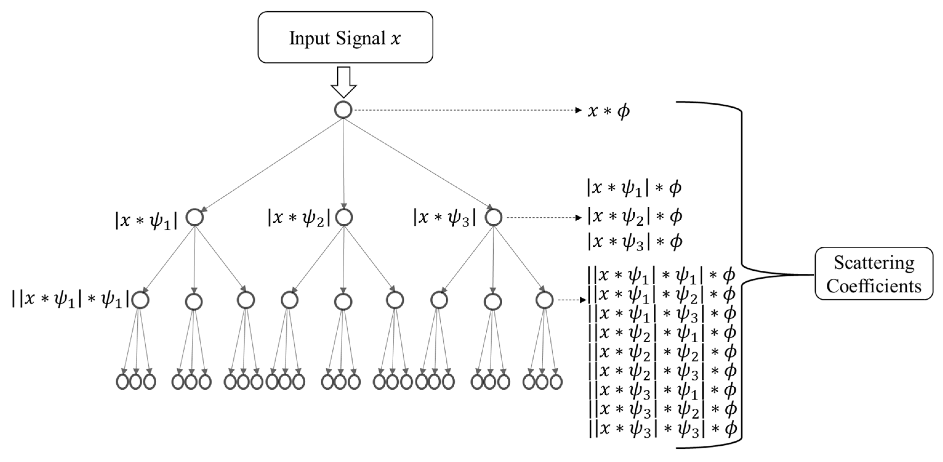
2.2. Wavelet Scattering Networks (WSNs)

In an effort to create interpretable networks that mimic human performance on vision and auditory tasks, some researchers use wavelet-transform-based methods, as wavelets are an approximation of the response of the human visual cortex and cochlea to stimuli [36]. For example, the wavelet transform renders a time domain signal to the time–frequency plane with a decreasing frequency resolution with increasing frequency, which is similar to the human cochlear response.

Mallat [37] proposed WSNs (Figure 1) as a first step in understanding the success of Convolutional Neural Networks (CNNs). A wavelet scattering network computes a representation that preserves high-frequency information, is stable to deformations, and is translation invariant, which makes it a good feature extractor for classification. It is a cascade (tree) of convolutions between Gabor wavelet transforms (represented by $\psi$ in Figure 1) and non-linear modulus and averaging operators (represented by $\varphi$ in Figure 1), which “scatter” the signal along multiple paths. The number of paths at each node of the WSN is the scale of the wavelet transform (scale = 3 in Figure 1), and the number of layers of wavelet transforms is typically two. Discrete versions of WSNs were proposed by Wiatowski [36] and involve existing discrete orthogonal and biorthogonal wavelets.

Unlike CNNs, a scattering network outputs coefficients at all layers, not just the last layer, and filters are not learned from data but are predefined wavelets. Thus, the filters retain their physical meaning, which cannot be said of the filters that are developed through the learning process in a typical convolution neural network. Operations in both CNNs and wavelet scattering networks can be represented as $P \left(\rho \left(x\ast w\right)\right)$, where $x$ is the input signal, $w$ is the filter weight, $\rho$ is the nonlinearity, and $P$ is the pooling operator. In CNNs, the weights $w$ are weights of learned random filters, while in WSNs, the weights $w$ are the weights of the fixed wavelet filters. Scattering networks provide state-of-the-art classification accuracies on simple to moderately complex datasets, such as textures in CUReT dataset [34], or musical genre and environmental sound classification [37], and images in MNIST dataset [38]. However, for extremely complex datasets such as ImageNet [39] or TIMIT Acoustic–Phonetic Continuous Speech Corpus [40], CNNs are still more accurate than scattering networks. A major reason for this is that scattering networks are fixed-feature generators, while CNNs learn features from the data. As a result, an effort is made to make the discrete wavelet scattering networks have the learnability property, such that they can learn features from the data.

2.3. Learnable Wavelet Scattering Networks (LWSNs)

Instead of the fixed wavelet filters of the WSN, the wavelet filters in the LWSN are learnable using a second-generation wavelet transform (SGWT). The classical wavelet transform is realized through the translation and expansion of the mother wavelet function. This definition is very restrictive, so the SGWT does away with it. The lifting method [35] or the lifting scheme (Figure 2) is a space domain wavelet construction method used to construct the SGWT filters, and it builds sparse representations by exploiting the correlation inherent in most real-world data. It consists of three basic steps:

• Split: Let $x\left(n\right)$ be an original signal. In this step, $x\left(n\right)$ is divided into two subsets: the even subset $x_e\left(n\right)$ and odd subset $x_o\left(n\right)$. The subsets are correlated according to the correlation structure of the original signal.

  $$x_e\left(n\right)=x\left(2n\right)$$

  (5)

  $$x_o\left(n\right)=x\left(2n+1\right)$$

  (6)
• Predict: The odd coefficients $x_o\left(n\right)$ are predicted from the neighboring even coefficients $x_e\left(n\right)$, and the prediction differences $d\left(n\right)$ are defined as the detail signal,

  $$d\left(n\right)=x_o\left(n\right)-P\left(x_e\left(n\right)\right)$$

  (7)

  where $P={\left[p\left(1\right),\cdots \cdots ,p\left(N\right)\right]}^T$ is the prediction operator.
• Update: Coarse approximation $c\left(n\right)$ to the original signal is created by combining the even coefficients and the linear combination of the prediction differences

  $$c\left(n\right)=x_e\left(n\right)+U\left(d\left(n\right)\right)$$

  (8)

  where $U={\left[u\left(1\right),\cdots \cdots ,u\left(N\right)\right]}^T$ is the update operator. By iterating on the approximation signal $c\left(n\right)$ using the three steps, the approximation and the detail signal are obtained at different levels. The optimization of the lifting scheme’s Update (U) and Predict (P) operators in the LWSN is carried out using the genetic algorithm (GA). The optimized Update (U) and Predict (P) operators are converted to the wavelet ($\psi$) and averaging operators ($\varphi$) using Claypoole’s algorithm [35], such that the structure in Figure 1 can be used to learn time–frequency representations from the data.

Table 1. Differences between networks.

	Deep Learning Networks	Wavelet Scattering Networks	Learnable Wavelet Scattering Networks
Features	Learnt from data	Fixed wavelet type and coefficients (not learnt from data)	Wavelet type and coefficients learnt from data
Features Output at	Last layer	Every layer	Every layer
Number of Layers	Variable number of hidden (convolutional) layers	Two layers (typically) of fixed wavelets	Two layers of learned wavelets
Nonlinearity	Modulus/Rectified Linear Unit/ Hyperbolic Tangent, etc.	Modulus	Modulus
Pooling	Max/Averaging, etc.	Averaging	Averaging
Learning Algorithm	Gradient Descent and Backpropagation	NA	Lifting method and genetic algorithm
Classifier	SoftMax	Any (e.g., SVM)	Any (e.g., SVM)
Architecture	Various architectures, e.g., ResNet [32] Alexnet [41], Recurrent Neural Network [42] etc.	See Figure 1	See Figure 1

illustrates the differences between deep learning networks, wavelet scattering networks, and learnable wavelet scattering networks.

2.4. Genetic Algorithm (GA)

The GA [43] mimics the theory of natural selection. As in the case with evolution, a population consists of individuals which reproduce to create the next generation. This reproduction involves the combination of genetic material from parents to create an offspring. Each subsequent generation will be created by parent individuals by combining their genes. The selection of parents (individuals) to combine is based on their fitness, and the fitness of an individual is based on the fitness function. A total of 10% of the individuals with the best fitness move on to the next generation. This mechanism is called elitism, and the percentage of the elite individuals can be changed. The remaining individuals take part in crossover, where the genes of two individuals (parents) are combined to create the genes of the individual of the next generation (child). Crossover is carried out until the required number of individuals (children) is created in the next generation. Analogous to mutation in natural reproduction, random changes are added to the genes of a fraction of the children created. This helps to avoid getting stuck in the local minima of the optimization of the fitness function. The process repeats for the new generation and the subsequent generations until the predefined maximum number of generations is reached or there is no improvement in the fitness in consecutive generations.

2.5. Support Vector Machine (SVM)

An SVM is based on the concept of finding decision planes or hyperplanes that maximize the separation between classes. If the classes are not linearly separable, a kernel trick is used to map the data into higher dimensions in an effort to separate them. To find the support vectors and hence construct an optimal hyperplane, the following optimization problem [44] is solved:

$$\begin{gathered} min\varphi \left(w\right)=\frac{1}{2}\Vert w{\Vert }^2+C{\displaystyle \sum }_{i=1}^N{\xi }_i \\ s.t.\hspace{1em}\hspace{1em}{y}_i\left(w^T\varphi \left(x_i\right)+b\right)\ge 1-{\xi }_i \end{gathered}$$

(9)

where $C$ is the penalty parameter to guard against overfitting, and ${\xi }_i$ are the slack variables introduced to handle inseparable data. The input data consists of $x_i$ and $y_i$, which are the independent and the dependent variable (class label), respectively. The kernel function $\varphi$ transforms the input data $x_i$into higher dimensions.

3. Fault Diagnosis Methodology

The implementation of the diagnostic scheme is depicted in Figure 3. Firstly, a dataset of signals when the circuit components are degrading is obtained via simulation or experimentation. This dataset is randomly split into a training dataset $\left[XTrain, YTrain\right]$ and a testing dataset $\left[XTest, YTest\right]$, where $XTrain$ and $Xtest$ represent the circuit output signals in the training and the testing dataset, respectively, and $YTrain$ and $YTest$ represent the corresponding labels (degrading components). A subset of signals (30%), ${XTrain}^{\prime }$, is randomly selected from the entire training dataset to be used with the GA. This is done to prevent overfitting to the training dataset and to reduce the time taken for GA optimization. The fitness function used is the Davies–Bouldin (DB) index [45], as it considers the ratio of within-class and between-class distances. As a result, the minimization of the DB index leads to maximum separation between the classes. The GA is used to optimize the Predict and Update operators of the SGWT, such that the DB index is minimized. The genes in each individual in the GA are the coefficients for the P and U operators that need to be optimized by the GA. The P and U operators are assumed to be of length 8; hence, the number of genes in each individual is 16. Other hyperparameters chosen for the GA include population size: 100, elite count: 10%, crossover fraction: 90%, mutation rate: 5%, and the stopping criterion of the GA is when there is no appreciable improvement in the fitness function for 30 consecutive generations. The feature space ($XTrainMod)$created by the LWSN, with the optimized P and U operators, is classified using the SVM as the classifier. Since SVM hyperparameter optimization is not the focus of this paper, the hyperparameter optimization was carried out using built-in MATLAB functions.

4. Experiments and Results

The proposed method was verified using two analog circuits, the Sallen–Key bandpass filter circuit and the two-switch forward convertor circuit, and two rotating machinery datasets, CWRU bearing faults dataset and UoC gear faults dataset. Fault data for the circuits is generated by varying component values around their nominal values within SPICE, i.e., if the nominal value of a component is Y, the lower range and the upper range of the deviation constituting the parametric fault of the component is [0.25 ∗ Y − 0.9 ∗ Y] and [1.1 ∗ Y − 1.75 ∗ Y], respectively. When the component value is between 0.9 ∗ Y and 1.1 ∗ Y, it is considered to be within its tolerance range, i.e., a tolerance range of 10%. The training data were obtained by conducting 1000 SPICE simulations, where components are varied in the aforementioned ranges one at a time, while the other components are held at their nominal values.

4.1. Sallen–Key Bandpass Filter

The first circuit under test (CUT1) is the Sallen–Key bandpass filter (Figure 4), which is the most frequently studied circuit for analog circuit fault diagnosis. Unlike other papers that only consider the fault diagnosis of four of the seven passive components, we considered all seven passive components for fault diagnosis. The parametric fault ranges for the seven components considered are shown in

Table 2. Nominal values and parametric fault range of Sallen–Key bandpass filter components.

Fault Class	Fault Code	Nominal Value	Faulty Range
Healthy	F0	NA	NA
$R_1$	F1	1 kΩ	[0.25 k 0.9 k] and [1.1 k 1.75 k]
$R_2$	F2	1 kΩ	[0.25 k 0.9 k] and [1.1 k 1.75 k]
$R_3$	F3	2 kΩ	[0.5 k 1.8 k] and [2.2 k 3.5 k]
$R_4$	F4	2 kΩ	[0.5 k 1.8 k] and [2.2 k 3.5 k]
$R_5$	F5	2 kΩ	[0.5 k 1.8 k] and [2.2 k 3.5 k]
$C_1$	F6	5 nF	[1.25 n 4.50 n] and [5.50 n 8.75 n]
$C_2$	F7	5 nF	[1.25 n 4.50 n] and [5.50 n 8.75 n]

. As can be seen from Table 2, we considered a single class for each component as opposed to other papers in the literature that consider two classes for each component. The data for each class were split into training and testing data sets via a 75%–25% split. The LWSN was trained on the training data, and the testing accuracy of the LWSN is reported in

Table 3. Fault diagnosis accuracy of LWSN and comparison with other methods.

Circuit	Literature (GB-DBN) [22]	Wavelet Scattering Networks	Proposed Method (LWSN)
CUT1	99.12%	90.01%	99.72%
CUT2	84.34%	82.45%	92.93%
CUT2 (Experimental Validation)	NA	81.12%	90.71%

, along with the testing accuracy of the original wavelet scattering network and the Gaussian–Bernoulli Deep Belief Network (GB-DBN)-based approach [22], which was used for comparison. This paper was used for comparison because it uses a deep-learning-based feature extractor, the DBN, along with an SVM for classification. Hence, it is conceptually similar to our paper. The confusion matrix for the fault diagnosis of the Sallen–Key bandpass filter using LWSN is shown in

Table 4. Confusion matrix for LWSN for Sallen–Key bandpass filter.

True Class	F0	99.4	0.6
	F1		99.8					0.2
	F2			99.8	0.2
	F3				100
	F4					100
	F5						100
	F6		1.8					98.2
	F7								100
		F0	F1	F2	F3	F4	F5	F6	F7
	Predicted Class

.

The Sallen–Key bandpass filter circuit involved seven fault types and one healthy class to detect and identify, which correspond to the 14 fault types for methods used in the literature. From Table 3, it can be seen that the proposed LWSN method achieved a marginal improvement of 0.7% in the fault diagnosis accuracy over comparable methods in the literature [18] and a 9% improvement in the fault diagnosis accuracy over a traditional WSN. As can be seen from the confusion matrix in Table 4, fault type F6, which corresponds to capacitor C1, was misdiagnosed most often; however, the diagnosis of other fault types was almost perfect.

4.2. Two-Switch Forward Convertor

The second circuit under test (CUT2) is the two-switch forward convertor circuit (Figure 5). A forward converter is a switching power supply circuit that is used for energy transfer when the two switches (transistors) are simultaneously turned on. The parametric fault ranges for the components considered after sensitivity analysis are shown in

Table 5. Nominal values and parametric fault range of two-switch forward convertor circuit components.

Fault Class	Fault Code	Nominal Value	Faulty Range	Experimental Values
Healthy	F0	NA	NA	NA
$R_1$	F1	33 Ω	[8.25 Ω 29.7 Ω] and [36.3 Ω 57.75 Ω]	10 Ω, 20 Ω, 40 Ω, 50 Ω
$C_4$	F2	0.1 μF	[0.025 μF 0.09 μF] and [0.11 μF 0.175 μF]	0.025 μF, 0.05 μF, 0.12 μF, 0.15 μF
$R_L$	F3	100 Ω	[25 Ω 90 Ω] and [110 Ω 175 Ω]	30 Ω, 80 Ω, 120 Ω, 170 Ω
$L_3$	F4	100 μH	[25 μH 90 μH] and [110 μH 175 μH]	30 μH, 75 μH, 156 μH, 170 μH
$R_5$	F5	0 Ω	[0.1 Ω 10 Ω]	2 Ω, 4 Ω, 6 Ω, 8 Ω
$R_6$	F6	0 Ω	[0.1 Ω 10 Ω]	2 Ω, 4 Ω, 6 Ω, 8 Ω
$R_7$	F7	0 Ω	[0.1 Ω 10 Ω]	2 Ω, 4 Ω, 6 Ω, 8 Ω
$R_8$	F8	0 Ω	[0.1 Ω 10 Ω]	2 Ω, 4 Ω, 6 Ω, 8 Ω
$R_{10}$	F9	0 Ω	[0.1 Ω 10 Ω]	2 Ω, 4 Ω, 6 Ω, 8 Ω
$R_{11}$	F10	0 Ω	[0.1 Ω 10 Ω]	2 Ω, 4 Ω, 6 Ω, 8 Ω
$R_{12}$	F11	0 Ω	[0.1 Ω 10 Ω]	2 Ω, 4 Ω, 6 Ω, 8 Ω
$R_{13}$	F12	0 Ω	[0.1 Ω 10 Ω]	2 Ω, 4 Ω, 6 Ω, 8 Ω
$R_{16}$	F13	0 Ω	[0.1 Ω 10 Ω]	2 Ω, 4 Ω, 6 Ω, 8 Ω
$R_L\ast C_4$	F14	100 Ω ∗ 10 μF	$\left($ ([0.025 μF 0.09 μF] and [0.11 μF 0.175 μF])	(30 Ω 0.025 μF), (30 Ω 0.175 μF), (170 Ω 0.025 μF), (170 Ω 0.175 μF)
$R_1\ast R_2$	F15	33 Ω ∗ 33 Ω	([8.25 Ω 29.7 Ω] and [36.3 Ω 57.75 Ω]) ∗	(10 Ω, 20 Ω), (10 Ω, 40 Ω), (30 Ω, 10 Ω), (50 Ω, 50 Ω),
			([8.25 Ω 29.7 Ω] and [36.3 Ω 57.75 Ω])
$R_2$	F16	33 Ω	[8.25 Ω 29.7 Ω] and [36.3 Ω 57.75 Ω]	10 Ω, 20 Ω, 40 Ω, 50 Ω

, along with the values for experimental verification. As can be seen from Table 5, we considered a single class for each single fault (single component degradation) as opposed to other papers in the literature that consider two classes for each single fault. The advantage of doing so is that we could consider one class for every double fault (two components degrading simultaneously), as can be seen from Fault Codes F14 and F15. If we were to consider two classes for each single fault, we would have to consider four classes for every double fault. The data for each class were split into training and testing data sets via a 75%–25% split. The testing accuracy of the LWSN on both the simulation and experimental data is reported in Table 3, along with the testing accuracy of the original wavelet scattering network and the Gaussian–Bernoulli Deep Belief Network (GB-DBN)-based approach [22], which were used for comparison. The confusion matrix for the fault diagnosis of the two-switch forward convertor circuit using LWSN is shown in

Table 6. Confusion matrix for LWSN for two-switch forward convertor circuit.

True Class	F0	91.7					0.7		3.5				0.5	3.5
	F1		94.4	0.2													5.3
	F2		0.5	89.9								9.6
	F3	0.8			78.4	3.8	0.8	1.3		14.0				0.8	0.3
	F4	0.5	0.3		1.6	89.7	0.3	5.7		0.5				0.8	0.8
	F5	0.3			0.3		98.2		0.5					0.5	0.3
	F6	0.5			1.2	3.9	1.2	92.0		0.2	0.2			0.5	0.2
	F7	3.1							94.8	0.3				1.3	0.5
	F8	0.2			14.4	2.0		0.5	0.7	81.9					0.2
	F9		0.3						0.3		99.2				0.3
	F10			9.9								88.3					1.8
	F11	1.0			0.3	0.3	0.8						97.1	0.3				0.3
	F12	4.2	0.2			1.0	1.7	0.2	1.0					90.3	1.2
	F13	0.5				0.5			0.2			0.2		0.2	98.3
	F14															100
	F15		4.1									0.7					94.9	0.3
	F16		4.7				2.3	2.3					2.3		4.7			83.7
		F0	F1	F2	F3	F4	F5	F6	F7	F8	F9	F10	F11	F12	F13	F14	F15	F16
	Predicted Class

.

The experimental setup that was used to demonstrate our approach is shown in Figure 6. The two-switch forward convertor circuit (CUT2) was used with pulse width waveforms to trigger the two switches, generated using an Agilent Arbitrary Waveform Generator 33250A. The circuit components were swapped out with the components with values shown in the Experimental values column of Table 5. For instance, to mimic the degradation of resistor R₁ from its nominal value of 33 Ω, resistors of 10 Ω, 20 Ω, 40 Ω, and 50 Ω were substituted, and the circuit output was captured at every instance. The circuit responses captured at the output using an Agilent Digital Oscilloscope 54853A were classified using the developed fault diagnosis methodology, and the results are provided in Table 3.

The sixteen fault types and one healthy class considered for the two-switch forward convertor correspond to 28 fault types for methods in the literature, and this is a much more challenging fault diagnosis problem compared to CUT1. From Table 3, it can be seen that the proposed LWSN method achieved a significant improvement of 8.9% in the fault diagnosis accuracy over the comparable method in the literature [22] and a 10.9% improvement in the fault diagnosis accuracy over the traditional WSN. As can be seen from the confusion matrix in Table 6, fault type F3, which corresponds to resistor R_L, was misdiagnosed as fault type F8 (resistor R8). Other notable misclassifications include the single fault F1 (resistor R1) and the double fault F15 (resistor R1 and R2). This highlights the complexity of analog circuit fault diagnosis. However, the developed LWSN method stands out in terms of fault diagnosis performance in comparison to existing methods.

4.3. Bearing Fault Diagnosis

In rotating machinery applications, rolling bearing faults are the most common, leading to the performance deterioration of machinery. Hence, bearing fault diagnosis plays a vital role in the health management of machinery [46]. To test the effectiveness of the method across different domains of fault diagnosis, the developed method was tested on a bearing faults benchmark dataset. The Case Western Reserve University (CWRU) motor bearing dataset was generated using a test rig consisting of a 2 hp Reliance Electric motor, a torque transducer/encoder, a dynamometer, and drive-end and fan-end Svenska Kullager-Fabriken deep-groove ball bearings. Inner ring, outer ring, and rolling element defects were manufactured into the bearings. The motor was run at a near-constant speed (1720–1797 r/min) with different loads (0–3 hp) provided by the dynamometer. Vibration data were collected using accelerometers, which were vertically attached to the housing with magnetic bases. Sampling frequencies were 12 kHz for some of the tests and 48 kHz for the others. Further details can be found at the CWRU Bearing Data Center website [47]. As shown in

Table 7. CWRU faults.

Fault Mode	Description
Health State	the normal bearing at 1791 rpm and 0 HP
Inner ring 1	0.007-inch inner ring fault at 1797 rpm and 0 HP
Inner ring 2	0.014-inch inner ring fault at 1797 rpm and 0 HP
Inner ring 3	0.021-inch inner ring fault at 1797 rpm and 0 HP
Rolling Element 1	0.007-inch rolling element fault at 1797 rpm and 0 HP
Rolling Element 2	0.014-inch rolling element fault at 1797 rpm and 0 HP
Rolling Element 3	0.021-inch rolling element fault at 1797 rpm and 0 HP
Outer ring 1	0.007-inch outer ring fault at 1797 rpm and 0 HP
Outer ring 2	0.014-inch outer ring fault at 1797 rpm and 0 HP
Outer ring 3	0.021-inch outer ring fault at 1797 rpm and 0 HP

, one healthy bearing and three fault modes, including the inner ring fault, the rolling element fault, and the outer ring fault, were classified into ten categories (one health state and nine fault states) according to different fault sizes. A plot of the data can be seen in Figure 7. The data were resampled such that the entire dataset had a constant sampling rate, and then, the data were split into chunks with sizes of 1024. The dataset was then split into training and testing datasets in the ratio of 75%:25% using stratified sampling. The LWSN achieved 99.2% accuracy for the testing dataset, which is comparable to the state-of-the-art methods [48]. The confusion matrix is shown in

Table 8. Confusion matrix for LWSN for the CWRU dataset.

True Class	Healthy	100.0
	Inner Ring 1		100.0
	Inner Ring 2			96.7	3.3
	Inner Ring 3				100.0
	Rolling Element 1					100.0
	Rolling Element 2						100.0
	Rolling Element 3							100.0
	Outer Ring 1								100.0
	Outer Ring 2	4.0								96.0
	Outer Ring 3										100.0
		Healthy	Inner Ring 1	Inner Ring 2	Inner Ring 3	Rolling Element 1	Rolling Element 2	Rolling Element 3	Outer Ring 1	Outer Ring 2	Outer Ring 3
	Predicted Class

.

The CWRU bearing dataset involves nine fault classes and one healthy class. As can be seen from the confusion matrix in Table 8, for the bearing fault diagnosis, fault types F3 and F9 were misdiagnosed most often; however, the diagnosis of other fault types was perfect.

4.4. Gear Fault Diagnosis

The second rotating machinery fault diagnosis dataset considered was the University of Connecticut (UoC) gear fault dataset [49]. The CWRU dataset and the UoC dataset were ranked the simplest and the most difficult benchmark dataset, respectively [48], for rotating machinery fault diagnosis. The average RMS and the average power of the signals in the CWRU and the UoC dataset were 0.27, −9.36 dB and 0.07, −21.91 dB, respectively. Preprocessing methods such as stochastic resonance [50] can be used to enhance weak fault characteristics in datasets such as UoC; however, in this paper, the LWSN method was applied directly to the raw vibration data.

In the UoC dataset, nine different gear conditions were introduced to the pinions on the input shaft, including healthy condition, root crack, missing tooth, spalling, and chipping tip with five different levels of severity. All the collected datasets were used and classified into nine categories (one health state and eight fault states missing, crack, spall, chip5a, chip4a, chip3a, chip2a, and chip1a) to test the performance. The data were resampled such that the entire dataset had a constant sampling rate, and then, the data were split into chunks with sizes of 1024. The dataset was then split into training and testing datasets in the ratio 75%:25% using stratified sampling. The LWSN achieved 96.51% accuracy for the testing dataset, and the confusion matrix is shown in

Table 9. Confusion matrix for LWSN for the UoC dataset.

True Class	Healthy	99.0	0.1	0.1	0.1	0.1	0.1	0.3
	Missing Tooth	0.3	98.6	0.3	0.3			0.3	0.1	0.1
	Root Crack	0.7	1.3	91.6	1.1	1.4	0.9	0.9	1.3	0.9
	Spalling	0.3			98.2	0.1	0.8		0.3	0.3
	Chipping Tip 1a	1.0	0.3	0.4	0.4	95.5	0.6	0.7	0.4	0.7
	Chipping Tip 2a	0.4	0.3	0.1		0.6	98.2		0.1	0.3
	Chipping Tip 3a	0.1		0.1	0.1	0.1	0.1	99.0	0.1	0.1
	Chipping Tip 4a	0.1		0.3	0.6	0.1	0.1	0.3	98.2	0.3
	Chipping Tip 5a	0.1						0.1	0.1	99.5
		Healthy	Missing Tooth	Root Crack	Spalling	Chipping Tip 1a	Chipping Tip 2a	Chipping Tip 3a	Chipping Tip 4a	Chipping Tip 5a
	Predicted Class

. Our result is marginally better, as the best result reported in [48] was 96.19%. Since the UoC dataset had 3600 samples per fault class and there were nine fault classes, the developed method is able to process the big data of rotating machinery.

4.5. Transfer Learning

In recent years, transfer learning has been gaining importance, as it enables knowledge acquired through training on data to be transferred from a source domain to gain insight in the target domain. This importance rises from the fact that it is very challenging to collect data from all possible conditions that machinery may encounter. Umdale et al. [51] created different datasets by dividing the original CWRU dataset based on speed and load, as can be seen in

Table 10. Comparison of transfer learning accuracies across different datasets.

Dataset	Source Dataset	Target Dataset	Training Accuracy [51]	Testing Accuracy [51]	Training Accuracy (LWSN)	Testing Accuracy (LWSN)
D1	1730 RPM and 3 HP 1750 RPM and 2 HP	1772 RPM and 1 HP 1797 RPM and 0 HP	97.22	97.02	100	99.96
D2	1772 RPM and 1 HP 1797 RPM and 0 HP	1730 RPM and 3 HP 1750 RPM and 2 HP	94.17	92.88	100	99.87
D3	1730 RPM and 3 HP 1797 RPM and 0 HP	1750 RPM and 2 HP 1772 RPM and 1 HP	96.92	95.77	100	99.39
D4	1750 RPM and 2 HP 1772 RPM and 1 HP	1730 RPM and 3 HP 1797 RPM and 0 HP	95.77	94.48	100	99.93

. For instance, in dataset D1, the goal was to determine if training on lower speeds in the source data set would still enable us to achieve acceptable fault diagnosis on a dataset with higher rotational speeds, as can be seen from the target dataset of D1. In dataset D2, the opposite was true—the goal was to determine if datasets with higher speeds would have vital information for fault diagnosis at lower speeds, whereas mixtures of speeds were considered in datasets D3 and D4. The maximum training and testing accuracies reported by [51] are shown in Table 10, where testing accuracies are an indication of the effectiveness of transfer learning. As can be seen from Table 10, the developed LWSN is more effective for transfer learning across all four datasets. Exploratory work suggests that LWSN can perform at least as well as deep learning networks at transfer learning, but further work needs to be undertaken to determine if there is a fundamental improvement.

These results imply that the LWSN network can extract discriminative information from raw data effectively and achieve fault classification with high accuracy, irrespective of the complexity and domain of the dataset.

5. Conclusions

Traditional fault diagnosis methods involve the extraction of fixed representations in the time domain, frequency domain, or time–frequency domain. These methods require technical expertise for designing appropriate features from the fixed representations. In this paper, a new feature extraction technique based on learnable wavelet scattering networks was developed to diagnose faults primarily in analog circuits and rotating machinery. By learning a time–frequency representation from the data, the developed method has a better ability to extract essential features of the fault signals. This results in better fault diagnosis accuracy, by almost 9%, compared to the state-of-the-art fault diagnosis method in the literature. By considering more classes for fault diagnosis than any other paper in the literature, a more thorough fault diagnosis was demonstrated. The fault diagnosis performance of this method was verified by experiments on the two-switch forward convertor circuit. The experiments indicated that the fault diagnosis model trained on simulation data is able to effectively diagnose faults from the actual circuit. Analog circuits and gears/bearings are the predominant sources of faults in electronic systems and rotary mechanical systems, respectively. The developed fault diagnosis approach was applied to the CWRU bearing faults and the UoC gear faults benchmark datasets and achieved fault diagnosis accuracy that is comparable to state-of-the-art methods. Since the UoC gear faults benchmark dataset is considered the most challenging benchmark dataset in rotating machinery fault diagnosis, this speaks to the ability of the developed method to extract weak fault signatures. Hence, the generalizability of the developed fault diagnosis approach across the most common industrial fault diagnosis domains was demonstrated. Initial experiments indicated that the developed approach is also effective in transfer learning; however, further experiments need to be carried out to confirm these observations.

The incorporation of learnability in traditional wavelet scattering networks resulted in a 10% improvement in fault diagnosis accuracy. As opposed to deep learning networks, the developed learnable wavelet scattering networks do not require an extensive trial-and-error process to optimize their structure. Additionally, the developed learnable wavelet scattering networks learn wavelet filters as opposed to the random filters learnt in deep learning networks. Hence, the filters learnt by learnable wavelet scattering networks are interpretable, which enables wavelets to be used to gain further insight into circuit faults. The interpretability of the wavelets learnt by the learnable wavelet scattering networks and digital circuit fault diagnosis are possible avenues for future research.

References

1. Pecht, M.; Jaai, R. A prognostics and health management roadmap for information and electronics-rich systems. Microelectron. Reliab. 2010, 50, 317–323. [Google Scholar] [CrossRef]
2. Binu, D.; Kariyappa, B.S. A survey on fault diagnosis of analog circuits: Taxonomy and state of the art. AEU-Int. J. Electron. Commun. 2017, 73, 68–83. [Google Scholar] [CrossRef]
3. Vasan, A.S.S.; Long, B.; Pecht, M. Diagnostics and prognostics method for analog electronic circuits. IEEE Trans. Ind. Electron. 2013, 60, 5277–5291. [Google Scholar] [CrossRef]
4. Yang, H.; Meng, C.; Wang, C. Data-driven feature extraction for analog circuit fault diagnosis using 1-D convolutional neural network. IEEE Access 2020, 8, 18305–18315. [Google Scholar] [CrossRef]
5. Li, F.; Woo, P.Y. Fault detection for linear analog IC—The method of short-circuit admittance parameters. IEEE Trans. Circuits Syst. I Fundam. Theory Appl. 2002, 49, 105–108. [Google Scholar] [CrossRef]
6. Tadeusiewicz, M.; Halgas, S.; Korzybski, M. An algorithm for soft-fault diagnosis of linear and nonlinear circuits. IEEE Trans. Circuits Syst. I Fundam. Theory Appl. 2002, 49, 1648–1653. [Google Scholar] [CrossRef]
7. Luo, H.; Wang, Y.; Lin, H.; Jiang, Y. Module level fault diagnosis for analog circuits based on system identification and genetic algorithm. Meas. J. Int. Meas. Confed. 2012, 45, 769–777. [Google Scholar] [CrossRef]
8. Cannas, B.; Fanni, A.; Montisci, A. Algebraic approach to ambiguity-group determination in nonlinear analog circuits. IEEE Trans. Circuits Syst. I Regul. Pap. 2010, 57, 438–447. [Google Scholar] [CrossRef]
9. Dai, X.; Gao, Z. From model, signal to knowledge: A data-driven perspective of fault detection and diagnosis. IEEE Trans. Ind. Inform. 2013, 9, 2226–2238. [Google Scholar] [CrossRef] [Green Version]
10. Bandyopadhyay, I.; Purkait, P.; Koley, C. Performance of a classifier based on time-domain features for incipient fault detection in inverter drives. IEEE Trans. Ind. Inform. 2019, 15, 3–14. [Google Scholar] [CrossRef]
11. Queiroz, L.P.; Rodrigues, F.C.M.; Gomes, J.P.P.; Brito, F.T.; Chaves, I.C.; Paula, M.R.P.; Salvador, M.R.; Machado, J.C. A fault detection method for hard disk drives based on mixture of gaussians and nonparametric statistics. IEEE Trans. Ind. Inform. 2017, 13, 542–550. [Google Scholar] [CrossRef]
12. Nasser, A.R.; Azar, A.T.; Humaidi, A.J.; Al-Mhdawi, A.K.; Ibraheem, I.K. Intelligent fault detection and identification approach for analog electronic circuits based on fuzzy logic classifier. Electronics 2021, 10, 2888. [Google Scholar] [CrossRef]
13. Shi, J.; Deng, Y.; Wang, Z. Analog circuit fault diagnosis based on density peaks clustering and dynamic weight probabilistic neural network. Neurocomputing 2020, 407, 354–365. [Google Scholar] [CrossRef]
14. Aizenberg, I.; Belardi, R.; Bindi, M.; Grasso, F.; Manetti, S.; Luchetta, A.; Piccirilli, M.C. A neural network classifier with multi-valued neurons for analog circuit fault diagnosis. Electronics 2021, 10, 349. [Google Scholar] [CrossRef]
15. Yuan, L.; He, Y.; Huang, J.; Sun, Y. A new neural-network-based fault diagnosis approach for analog circuits by using kurtosis and entropy as a preprocessor. IEEE Trans. Instrum. Meas. 2010, 59, 586–595. [Google Scholar] [CrossRef]
16. Xiao, Y.; He, Y. A novel approach for analog fault diagnosis based on neural networks and improved kernel PCA. Neurocomputing 2011, 74, 1102–1115. [Google Scholar] [CrossRef]
17. Xiao, Y.; Feng, L. A novel linear ridgelet network approach for analog fault diagnosis using wavelet-based fractal analysis and kernel PCA as preprocessors. Meas. J. Int. Meas. Confed. 2012, 45, 297–310. [Google Scholar] [CrossRef]
18. Zhang, A.; Chen, C.; Jiang, B. Analog circuit fault diagnosis based UCISVM. Neurocomputing 2016, 173, 1752–1760. [Google Scholar] [CrossRef]
19. Song, P.; He, Y.; Cui, W. Statistical property feature extraction based on FRFT for fault diagnosis of analog circuits. Analog Integr. Circuits Signal Process. 2016, 87, 427–436. [Google Scholar] [CrossRef]
20. He, W.; He, Y.; Li, B.; Zhang, C. Analog circuit fault diagnosis via joint cross-wavelet singular entropy and parametric t-SNE. Entropy 2018, 20, 604. [Google Scholar] [CrossRef] [Green Version]
21. Cui, J.; Wang, Y. A novel approach of analog circuit fault diagnosis using support vector machines classifier. Meas. J. Int. Meas. Confed. 2011, 44, 281–289. [Google Scholar] [CrossRef]
22. Liu, Z.; Jia, Z.; Vong, C.M.; Bu, S.; Han, J.; Tang, X. Capturing high-discriminative fault features for electronics-rich analog system via deep learning. IEEE Trans. Ind. Inform. 2017, 13, 1213–1226. [Google Scholar] [CrossRef]
23. Zhao, G.; Liu, X.; Zhang, B.; Liu, Y.; Niu, G.; Hu, C. A novel approach for analog circuit fault diagnosis based on Deep Belief Network. Meas. J. Int. Meas. Confed. 2018, 121, 170–178. [Google Scholar] [CrossRef]
24. Chen, P.; Yuan, L.; He, Y.; Luo, S. An improved SVM classifier based on double chains quantum genetic algorithm and its application in analogue circuit diagnosis. Neurocomputing 2016, 211, 202–211. [Google Scholar] [CrossRef]
25. Wenxin, Y. Analog circuit fault diagnosis via FOA-LSSVM. Telkomnika 2020, 18, 251. [Google Scholar] [CrossRef]
26. Liang, H.; Zhu, Y.; Zhang, D.; Chang, L.; Lu, Y.; Zhao, X.; Guo, Y. Analog circuit fault diagnosis based on support vector machine classifier and fuzzy feature selection. Electronics 2021, 10, 1496. [Google Scholar] [CrossRef]
27. Gao, T.Y.; Yang, J.L.; Jiang, S.D.; Yang, C. A novel fault diagnostic method for analog circuits using frequency response features. Rev. Sci. Instrum. 2019, 90, 104708. [Google Scholar] [CrossRef]
28. He, W.; He, Y.; Li, B.; Zhang, C. A naive-Bayes-based fault diagnosis approach for analog circuit by using image-oriented feature extraction and selection technique. IEEE Access 2020, 8, 5065–5079. [Google Scholar] [CrossRef]
29. He, W.; He, Y.; Luo, Q.; Zhang, C. Fault diagnosis for analog circuits utilizing time-frequency features and improved VVRKFA. Meas. Sci. Technol. 2018, 29, 045004. [Google Scholar] [CrossRef]
30. Ji, L.; Fu, C.; Sun, W. Soft fault diagnosis of analog circuits based on a ResNet with circuit spectrum map. IEEE Trans. Circuits Syst. I Regul. Pap. 2021, 68, 2841–2849. [Google Scholar] [CrossRef]
31. Khemani, V.; Azarian, M.H.; Pecht, M.G. Electronic circuit diagnosis with no data. In Proceedings of the 2019 IEEE International Conference on Prognostics and Health Management (ICPHM), San Francisco, CA, USA, 17–20 June 2019; pp. 1–7. [Google Scholar] [CrossRef]
32. He, K.; Zhang, X.; Ren, S.; Sun, J. Deep residual learning for image recognition. In Proceedings of the IEEE Computer Society Conference on Computer Vision and Pattern Recognition, Las Vegas, NV, USA, 27–30 June 2016. [Google Scholar]
33. Elsken, T.; Metzen, J.H.; Hutter, F. Simple and efficient architecture search for convolutional neural networks. In Proceedings of the 6th International Conference on Learning Representations, ICLR 2018—Workshop Track Proceedings, Vancouver, BC, USA, 30 April–3 May 2018. [Google Scholar]
34. Bruna, J.; Mallat, S. Invariant scattering convolution networks. IEEE Trans. Pattern Anal. Mach. Intell. 2013, 35, 1872–1886. [Google Scholar] [CrossRef] [Green Version]
35. Sweldens, W. The lifting scheme: A construction of second generation wavelets. SIAM J. Math. Anal. 1998, 29, 511–546. [Google Scholar] [CrossRef] [Green Version]
36. Wiatowski, T.; Tschannen, M.; Stanic, A.; Grohs, P.; Bolcskei, H. Discrete deep feature extraction: A theory and new architectures. In Proceedings of the 33rd International Conference on Machine Learning, New York, NY, USA, 19–24 June 2016; Volume 5, pp. 3168–3183. [Google Scholar]
37. Andén, J.; Lostanlen, V.; Mallat, S. Joint time-frequency scattering. IEEE Trans. Signal Process. 2019, 67, 3704–3718. [Google Scholar] [CrossRef] [Green Version]
38. LeCun, Y.; Cortes, C.; Burges, C. The MNIST Database of Handwritten Digits. Courant Inst. Math. Sci. 1998. Available online: http://yann.lecun.com/exdb/mnist/ (accessed on 25 January 2022).
39. Deng, J.; Dong, W.; Socher, R.; Li, L.-J.; Li, K.; Li, F.-F. ImageNet: A large-scale hierarchical image database. In Proceedings of the 2009 IEEE Conference on Computer Vision and Pattern Recognition, Miami, FL, USA, 20–25 June 2009. [Google Scholar]
40. Garofolo, J.S.; Lamel, L.F.; Fisher, W.M.; Fiscus, J.G.; Pallett, D.S.; Dahlgren, N.L.; Zue, V. TIMIT Acoustic-Phonetic Continuous Speech Corpus; Linguistic Data Consortium: Philadelphia, PA, USA, 1993. [Google Scholar]
41. Krizhevsky, A.; Sutskever, I.; Hinton, G.E. ImageNet classification with deep convolutional neural networks. In Proceedings of the Advances in Neural Information Processing Systems, Lake Tahoe, NV, USA, 3–6 December 2012. [Google Scholar]
42. Hochreiter, S.; Schmidhuber, J. Long short-term memory. Neural Comput. 1997, 9, 1735–1780. [Google Scholar] [CrossRef]
43. Holland, J.H. Genetic Algorithms. Sci. Am. 1992, 267, 66–73. [Google Scholar] [CrossRef]
44. Cortes, C.; Vapnik, V. Support-vector networks. Mach. Learn. 1995, 20, 273–297. [Google Scholar] [CrossRef]
45. Davies, D.L.; Bouldin, D.W. A cluster separation measure. IEEE Trans. Pattern Anal. Mach. Intell. 1979, PAMI-1, 224–227. [Google Scholar] [CrossRef]
46. Mao, W.; Wang, L.; Feng, N. A new fault diagnosis method of bearings based on structural feature selection. Electronics 2019, 8, 1406. [Google Scholar] [CrossRef] [Green Version]
47. Bearing Data Center|Case School of Engineering|Case Western Reserve University. Available online: https://engineering.case.edu/bearingdatacenter (accessed on 25 January 2022).
48. Zhao, Z.; Li, T.; Wu, J.; Sun, C.; Wang, S.; Yan, R.; Chen, X. Deep learning algorithms for rotating machinery intelligent diagnosis: An open source benchmark study. ISA Trans. 2020, 107, 224–255. [Google Scholar] [CrossRef]
49. Gear Fault Data. Available online: https://figshare.com/articles/dataset/Gear_Fault_Data/6127874/1 (accessed on 25 January 2022).
50. Qiao, Z.; Elhattab, A.; Shu, X.; He, C. A second-order stochastic resonance method enhanced by fractional-order derivative for mechanical fault detection. Nonlinear Dyn. 2021, 106, 707–723. [Google Scholar] [CrossRef]
51. Udmale, S.S.; Singh, S.K.; Singh, R.; Sangaiah, A.K. Multi-fault bearing classification using sensors and ConvNet-based transfer learning approach. IEEE Sens. J. 2020, 20, 1433–1444. [Google Scholar] [CrossRef]
Figure 1. Wavelet scattering network.
Electronics 11 00451 g001
Figure 2. Lifting scheme.
Electronics 11 00451 g002
Figure 3. Fault diagnosis methodology.
Electronics 11 00451 g003
Figure 4. Sallen–Key bandpass filter.
Electronics 11 00451 g004
Figure 5. Two-switch forward convertor circuit.
Electronics 11 00451 g005
Figure 6. Experimental setup for demonstrating the developed approach.
Electronics 11 00451 g006
Figure 7. Vibration signals of the different faults in the CWRU dataset.
Electronics 11 00451 g007