1. Introduction
Autism spectrum disorder (ASD) is a neurodevelopmental disorder that affects children who manifest heterogeneous characteristics, such as differences in behaviour, problems communicating with others and social disabilities [
1]. According to the World Health Organization, ASD affects one in 160 children worldwide [
2]. It also appears in childhood and persists into adulthood. Many symptoms of ASD appear, such as genetic, cognitive, neurological and cognitive factors [
3]. These symptoms appear in childhood but the diagnosis of ASD is not made until 2–3 years after the onset of symptoms, usually at the age of 4 years [
4]. Detecting autism is a difficult task that requires effort and a long period to improve cases. For early detection of autism, many behavioural and physiological techniques have been used to identify autism effectively and accurately in children [
5]. Predictive indicators to inform parents of the behaviour, physiological status and course of their children very early are also needed, along with informing scientific research centres about finding appropriate solutions and treatments.
Although clinical and physiological characteristics are not identified early, some of the vital behavioural characteristics have a high ability to determine autism and its degree. Eye-tracking technology is one of the most important and promising indicators for ASD because it is fast, inexpensive, easy to analyse and applicable to all ages. Eye movement tracking is an investigational procedure that generates, tracks and captures points and calculates eye movement through these points. Many studies have demonstrated that eye movements have a strong effect on the response to visual and verbal cues as biomarkers of ASD [
6]. Some studies have also shown that early detection of ASD by tracking eye movements has correlations with clinical testing [
7]. Some of these correlations are due to genetic factors [
8]. In addition, diagnosis by eye tracking is useful in short-term detection of children with ASD.
Eye tracking is a sensitive tool for examining behaviour and customising eyesight to process a range of information about visual stimuli [
9]. In previous years, researchers focused on diagnosing ASD through eye tracking and on the biological and behavioural patterns of eye movement, especially in children exposed to multiple developmental disorders, including ASD [
10]. Eye-tracking technology, as a biomarker for assessing children with autism, has many advantages. Firstly, it provides ease of eye tracking for young children, which means early detection of autism risks. Secondly, eye-tracking data provide a range of information that is used as biomarkers, which indicate atypical visual focus [
11]. Thirdly, eye-tracking technology is an easy and straightforward measure that is related to the screening tools used to diagnose ASD [
12]. Thus, eye-tracking models that measure non-social and social orientation performance have significant correlations in ASD. These models take advantage of social attention deficits to detect ASD at an early age. However, evidence regarding positive eye-tracking outcomes as a strong predictor of long-term outcomes in children with ASD is lacking.
One of the greatest challenges in ASD is the heterogeneous response to treatment and the search for effective treatments to improve responses in children with autism. From this point, researchers and experts have set out a search for the development of new treatment methods that target children who are less responsive to the currently available treatment methods. In this study, the developed artificial intelligence systems to enhance the early detection of autism disease in an eye-tracking dataset containing two classes showed that children in the first class tend to show lower social visual attention (SVA) than second-class typical development (TD).
The major contributions in this work are as follows:
This research aimed to diagnose an ASD dataset and distinguish cases of autism from cases of TD.
This research also aimed to enhance images, remove all noises from the eye-tracking path area and extract the paths of eye points falling on the image, with high efficiency using overlapping filters.
The most important representative features from the areas of the eye tracks were extracted using local binary pattern (LBP) and grey level co-occurrence matrix (GLCM) algorithms. The features of the two methods were merged into one vector, called hybrid, and classified using two classifiers, FFNN and ANN.
The dataset was balanced; also, the parameters of the GoogleNet and ResNet-18 deep learning models were adjusted and modified to extract the deep feature maps for diagnosing autism with high efficiency.
A hybrid technology between deep learning models (GoogleNet and ResNet-18) and machine learning algorithms (SVM) was developed to obtain superior results for ASD diagnosis.
Artificial intelligence techniques, namely, machine learning, deep learning and hybrid techniques, could help experts and autism treatment centres in the early detection of autism in children.
The rest of the paper is organised as follows:
Section 2 describes a set of relevant previous studies.
Section 3 shows the analysis of the materials and methods for the ASD dataset, and contains subsections for three proposed systems.
Section 4 presents the results achieved by machine learning, deep learning and the hybrid technique between them.
Section 5 provides discussion and comparison between the proposed systems.
Section 6 concludes the paper.
2. Related Work
Here, a set of recent relevant previous studies is reviewed.
Lord. et al. presented a method called autism diagnostic observation schedule for assessing autism. It is a set of features and unstructured observational tasks in which the doctor evaluates the response of children through some desirable and undesirable situations, with a focus on behaviour that indicates autism [
12]. Schopler et al. presented a scale for assessing autism through the child autism rating scale, which is based on the doctor’s assessment of children’s behaviour through two scales, a social communication questionnaire and a social responsiveness scale; it is a more reliable measure according to opinions [
13]. Moore. et al. introduced a system for tracking eye data, extracting features and training them on machine learning classifiers. The study was applied to 71 people divided into 31 with autism and 40 controls. The authors used different stimuli to evaluate the performance of the system. The system achieved an accuracy of 74% [
14]. Thorup et al. presented two eye-tracking behaviours, namely, referential looking and joint attention, for autism detection.
Recent studies using dynamic stimuli indicated a difference between eye and head movement during the application of joint attention tasks; this difference is a unique characteristic of people with autism. The results concluded that relying on the eye and the head signal is better than relying on eye movement. Eye movement tracking is a powerful visual attention assessment tool for understanding the behaviour of people with autism [
15]. Jones et al. investigated differential attention and visual fixation with characteristic features of visual stimuli. They focused on distinguishing between children with ASD and those without, rather than determining the severity of the autism spectrum [
16]. Bacon et al. revealed that biomarkers, such as genetics, physiological behaviour, neurodevelopment and eye tracking, contribute to the diagnosis of autism. Eye tracking was used to assess social stimuli in several samples, such as children with ASD, Down syndrome, Rett syndrome and Williams syndrome [
17].
Mazumdar et al. presented a method that was based on extracting and classifying eye-tracking features through machine learning algorithms. The features were extracted from display behaviour, image content and scene centres. The system achieved high performance in distinguishing children with autism spectrum from typically developing children [
18]. Belen et al. presented the EyeXplain Autism method that enables clinicians to track eyes, analyse data and interpret data extracted by DNN [
19]. Oliveira et al. proposed a computational method that was based on integrating the concepts of visual attention and artificial intelligence techniques through the analysis of eye-tracking data. These data were categorised by a machine learning algorithm and the system reached an accuracy of 90% [
20]. Li et al. proposed a sparsely grouped input variables for neural network (SGIN) method for identifying stimuli that differentiate grouping with clinical features [
21]. Yaneva et al. presented an approach to detecting autism in adults by eye-tracking. Eye movements were recorded, and machine learning algorithms were trained to detect autism. Effects were detected based on eyesight and other variables. The system achieved an accuracy of 74% [
22].
3. Materials and Methods
In this section, techniques, methods and materials for evaluating an ASD dataset were analysed, as shown in
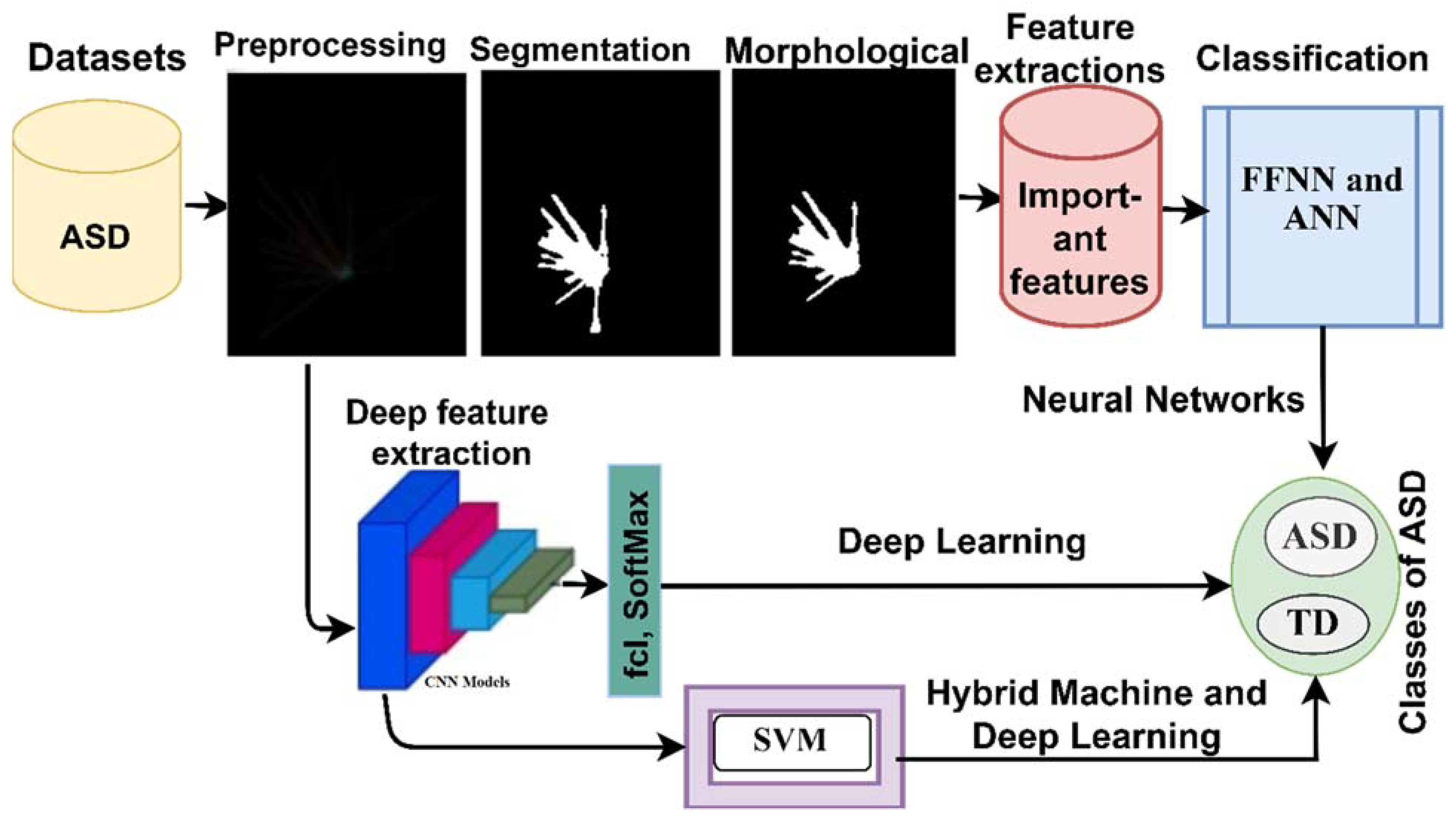
Figure 1. Data were collected from patients with autism spectrum disorder and others developing it. All images were subjected to pre-processing. After optimised images were obtained, three techniques were applied. Firstly, a Neural Networks technique based on extracting features from the segmented eye-tracking area was applied using a snake model. Then, features were extracted by LBP and GLCM hybrid methods. Subsequently, the features of the two methods were combined into one vector for each image and diagnosed using ANN and FFNN algorithms. The second technique for detecting ASD used convolutional neural network (CNN) models, such as GoogleNet and ResNet-18. The third technique was a hybrid technique between the two techniques of machine learning (SVM) and deep learning (GoogleNet and ResNet-18), which are called GoogleNet + SVM and ResNet-18 + SVM, one of the contributions of this study.
3.1. Dataset
In this work, the dataset from the Figshare data repository was used; these images were collected and prepared by Carette et al. [
23]. The dataset contains 547 images of children divided into two classes: ASD, which contains 219 images, and TD, which contains 328 images. In addition, images were collected from 59 children as follows: 29 children with ASD (25 males and 4 females) and 30 children with TD (13 males and 17 females) [
24].
Figure 2 depicts samples from ASD and TD dataset.
3.2. Average and Laplacian Filters
Most images contain noise caused by many factors, whether when taking images or storing them. This noise must be treated to obtain important and accurate features. Image optimisation is the first step in image processing to repair damaged features that have an effect on the diagnostic process. Several filters are used to enhance images, remove noise and increase edge contrast. In this work, all images were enhanced by average and Laplacian filters. Firstly, an average filter was applied to all the images. The filter works at a size of 5 × 5 and keeps moving on the image until the whole image is processed and smoothed by reducing the differences between the different pixels and replacing each central pixel, with the average value of the adjacent 24 pixels. Equation (1) describes the mechanism of how to smooth an image with an average filter [
25].
where
f(
L) is the enhanced image (output),
y(
L − 1) is the previous input and
L is the number in the average filter.
Secondly, a Laplacian filter, which detects edges and shows the edges of scenes taken from eye tracking, was applied. Equation (2) shows how the Laplacian filter works on the image.
where
f represents a second-order differential equation and
x,
y is the coordinate in a two-dimensional matrix.
Finally, a fully optimised image was obtained by subtracting the image optimised by the Laplacian filter from the resultant image by the average filter, as in Equation (3).
Figure 2b shows some samples of the data set after the enhancement process.
All images were enhanced to be inputted into the following three proposed systems.
3.3. First Proposed System Using Neural Networks Techniques
3.3.1. Snake Algorithm (Segmentation)
The snake algorithm is one of the latest algorithms for appropriate segmentation and identification of the region of interest (ROI) and isolation of it from the rest of the image for further analysis. The algorithm moves along the edges of the ROI, where the ∁ curve is represented by setting the function
: Ω → and the model starts with zero at the first boundary region of the ROI
I [
26]; Ω → represents the lesion region. The curve ∁ divides each subregion
fk Ω into two subregions inside and outside
f,
f with
, as shown in Equation (4), where
represents sub-regions belonging to the Ω (lesion region).
The snake model begins by a growing contour inward. ROI boundaries are determined by a first contour determination and eye-tracking scene map calculation. The model moves within the ROI boundary when > 0 is set, whilst the area outside the ROI is calculated by subtracting the currently calculated subregion from the previously calculated subregion, as shown in Equation (5).
The outer sub-area is calculated using Equation (6).
The segmentation algorithm is applied by the snake model that moves toward the boundary of the object through the external energy that moves toward the boundary of the object when the level is set to zero. The following Equation (7) describes the energy function of the
function.
where
is constant and
. The terms
are defined in Equations (8) and (9).
where
Hε (
) indicates the Heaviside function and
δε (
) indicates the univariate Dirac delta function. When the zero level
C curve is pushed to a smooth plane,
Lspq (
) is reduced. The energy in
spq(
I) speeds up moving curves and defines the boundaries of a scene for eye tracking. The parameter v of
Aspq (
) is a positive or negative value that depends on where the snake model is in an ROI. When the value of v is positive, the snake model is located outside the ROI and if the value of v is negative, the snake model is located inside the ROI to speed up the determination of the scene region. The
spq(
I) function is a mathematical expression that has two values [1, −1], either inside or outside an ROI. When set to a value of 1, the snake model is outside the object and modifies the compressive force to shrink the contour, and when set to −1, the contour expands when inside the object, as shown in Equation (10).
The
function and
function are the smoothed part of the entire image, as calculated using Equations (11) and (12).
An algorithm stops when the pixel value is similar between two consecutive contours and this point is called the algorithm stop point, as in Equation (13).
If
then the snake model stops running.
Here,
indicates the last computed mask for the snake model;
refers to the new mask of the snake model; and row and col are the max numbers in the images. The model stops moving between the value ranges of 98 and 100 obtained by calculating the average intensity of the initial contour.
Figure 3 describes samples from the dataset after segmentation and ROI by the eye-tracking path.
3.3.2. Morphological Method
The morphological method is a method for further image optimisation after segmentation. After the fragmentation process, holes that do not belong to the ROI are left. Thus, these holes must be removed. Many morphological methods, such as erosion, dilation, and opening and closing, create structural elements of a specific size, move them to every position of the image and replace the target pixel with suitable pixels on the basis of adjacent pixels. In this study, two methods were used. The first method is the adjacent union test, which is called ‘fits’. The second method, called ‘hits’, tests the adjacent intersection. The morphological processes produced improved binary images, as shown in
Figure 4, which illustrates samples of the dataset before and after the morphological process [
27].
3.3.3. Feature Extraction
In this work, the most important representative features from the ROI were extracted by two algorithms, LBP and GLCM. Then, the extracted features from the two algorithms were combined with each other to produce strong representative features. Extracting the features from several methods and combining them are two of the most important recent methods that have an effect on accurate diagnosis. The LBP algorithm is one of the methods to extract features. In this study, the LBP was set to a size of 4 × 4. The method selects the central pixel (
) one at a time and determines the neighboring pixels (
), which are 15 pixels, and replaces the central pixel with adjacent pixels in accordance with Equation (14). Thus, each central pixel was replaced by adjacent pixels and the process was repeated until all pixels were replaced by the image; 203 features were extracted for each image.
where
P represents the number of pixels in the image and the binary threshold
is determined as in Equation (15).
The features were then extracted by the GLCM algorithm, which showed different levels of grey levels in the ROI. The algorithm extracted features from the region of the eye-tracking track. The algorithm collected spatial information that determines the relationship between the centre pixel and adjacent pixels in accordance with distance d and angle θ. The four representations of the angle are 0°, 45°, 90° and 135°, and the value of d is either 1 when the angle is θ = 0° or θ = 90° or the value of d = √2 when the angle is θ = 45° or θ = 135°. The GLCM algorithm produced 13 essential features for each image.
Figure 5 describes the hybridisation of features extracted by the LBP and GLCM algorithms.
3.3.4. Classification
In this section, the ASD dataset was evaluated based on two neural network algorithms, namely, an ANN and an FFNN.
ANN and FFNN Algorithms
An ANN is a computerised neural network that consists of an input layer with many neurons in it; many hidden layers in which interconnected neurons are carried out and where many complex arithmetic operations are performed to solve the problems to be solved; and an output layer that contains neurons with the same number of classes to be classified [
28]. The algorithm analyses and interprets many large and complex data to produce clear patterns. Each neuron is associated with the other by specific w weights that have a role in reducing the error between the predicted and actual output. The ANN algorithm updates the weights in each iteration until a minimum squared error is obtained between the actual output X and the predicted Y, as described by Equation (16).
where N is the number of data points.
In this study, an ANN was evaluated on the ASD dataset. A total of 216 features (neural cells) were inputted into the input layer, trained through 10 interconnected hidden layers with certain weights, and then fed to the output layer that contains two classes (neural), ASD and TD.
Figure 6 describes the ANN architecture of the ASD dataset, in which 216 features were entered and processed through 10 layers and two classes were produced.
An FFNN is a computational neural network for solving complex problems similar to the structure of the ANN algorithm in the input layer, hidden layers and the output layer. All neurons in the hidden layers are interconnected from one layer to the other by connections called weights w. The working mechanism of the algorithm is to feed the neurons in the forward direction called the forward stage, where the neurons are fed in the forward direction, and the output of each neuron is calculated on the basis of the weights obtained from the previous neuron. In other words, the weights are adjusted and updated from the hidden layer to the output layer [
29]. The minimum squared error is calculated between the actual and predicted output and the process continues until the minimum error is obtained as in the above equation.
3.4. CNN Models
CNNs are a modern technique and type of neural network, which arises as a multi-layered perceptual diversity. They are designed to process two-dimensional data, especially medical images and audio signals, into spectrum charts, and can also be modified and adapted to perform tasks in one or several dimensions. The idea began to develop with Kunihiko Fukushima, who in 1982 developed the recognition system, a backpropagation neural network that mimics the process of the visual cortex [
30].
A convolution layer is a kind of linear operation between the filter and the image; in other words, it is the operation of two functions,
x(
t) and
w(
t), denoted by (x ∗ w)(t) or s(t) as Equation (17). There are three important parameters for convolutional layers which are the filter, the p-step, and zero-padding.
x(t) is the input, w(t) is the filter, and s(t) is the output of the convolutional layer called the deep feature map. If t is an integer value and w is defined only with integer values, then as Equation (18):
One of the essential things that we must keep in mind when implementing a CNN is the dimension of the input images or signals, we are working on, which the filter must adapt to the necessary dimensions of the input (in the case of colour images it is three dimensions, in the case of black and white two-dimensional images). In the case of two dimensions, the convolution formula, with the input I and with kernel K, is as Equation (19):
Colour images have three dimensions, including three two-dimensional layers (RGB channels). In this case, convolution layers consist of three 2D convolutions, one for the red layer R, one for the green layer G, and one for the blue layer B, and adding the results. One problem with p-step convolution is matching the input dimensions to the base dimension. One of the solutions is the zero-padding process (filling with zeros), to increase the input dimensions; the zero padding is adding a column of zeros to the right, left, bottom or top when necessary and as needed. Usually, the dimensions of the resulting convolution operation are less than the first input, which is why the zero-padding operation is used to equalise the dimensions, or it is handled by preserving the input edges of the original image. A convolutional layer consists of implementing multiple convolutions, adding bias values to all inputs, and obtaining deep feature maps [
31].
After convolutional layer operations, ReLU (Rectified Linear Unit) layers are used for further processing of the input. The purpose of this layer is to pass positive values and suppress negative values and convert them to zero. Equation (20) describes the working mechanism of the ReLU layer.
Convolutional layers produce millions of parameters that cause overfitting. A dropout layer, which stops 50% of the neurons in each iteration and passes the other 50% and so on, is used to solve this problem. In the present work, this percentage was manually set to 50%. However, this layer doubled the training time of the network.
After a convolutional layer is executed, it produces large dimensions. For the acceleration process, reducing the dimensions is necessary and this task is performed by pooling. Pooling layers interact inside the CNN in the same manner as the convolutional layer and they perform small operations in the input matrix areas. Pooling layers have two methods for reducing dimensions: max pooling and average pooling. In the max pooling method, the max value is chosen from amongst the set of values specified in the matrix, as described in Equation (21). In the average pooling method, the set of values specified in the matrix is averaged and the matrix is represented by the average value, as described in Equation (22).
where
A is represents the matrix;
m,
n are dimensions of the matrix,
k is the matrix amplitude and
p are the stride.
The last layer in CNNs is the fully connected layer. This layer is characterised by the connection of each neuron with the other neurons. In this layer, the deep feature maps are converted from 2D to a 1D (unidirectional) representation. This layer is responsible for classifying all the inputted into the appropriate classes. The number of connected layers varies from one CNN model to another and more than one fully connected layer could be used in the same network. CNN models take a long time to train. The last fully connected layer is the SoftMax activation function, which is a non-linear function that produces two classes, DSA and TD, for the ASD dataset. Equation (23) describes how the SoftMax function works.
y(x) represents the SoftMax function, with a value between .
This section focuses on two CNN models, GoogLeNet and ResNet-18.
3.4.1. CNN GoogLeNet Model
The GoogLeNet model is a type of CNN used for classification, pattern recognition, and many computer vision tasks. The network contains 22 deep layers (27 layers, including pooling layers). It is distinguished by its computational efficiency and greatly reducing its dimensions whilst preserving important information. The first convolutional layer works with a 7 × 7 filter, which is large compared to the sizes of other filters and greatly reduces the dimensions of the input images. All 49 pixels are represented by one pixel whilst preserving the important information. The second convolutional layer reduces the dimensions (size) of the image. The network has three max pooling layers with the size of 3 × 3 that down-sample the input dimensions by reducing the height and width of the image. GoogLeNet also contains one average pooling layer with a size of 7 × 7 that significantly reduces the dimensions of the input image [
32]. GoogLeNet contains 7 million parameters as describes in
Table 1.
Figure 7 describes the GoogLeNet infrastructure for diagnosing ASD.
3.4.2. CNN ResNet-18 Model
The ResNet-18 model is a type of deep feature extraction CNN. ResNet-18 belongs to the ResNet-xx family of networks. The ResNet-18 network consists of 18 deep layers divided into five convolutional layers for extracting deep feature maps, a ReLU layer, one average pooling layer for reducing image dimensions and a fully connected layer for converting feature maps from 2D to 1D and classifying all inputted images represented by feature vectors into their appropriate class [
33]. The softMax activation is a function that classifies the dataset into two classes, ASD and TD.
Figure 8 describes the architecture of the ResNet-18 model, which contains many layers and more than 11.5 million parameters as described in
Table 2.
3.5. Hybrid of Deep Learning and Machine Learning
This section describes a new technique, which is a hybrid technique between machine learning and deep learning networks, for the early detection of ASD. In deep learning, models require highly efficient hardware resources and consume a long time to train the dataset. Thus, to solve these challenges, hybrid techniques are used [
34]. They require medium-efficient hardware resources and they do not consume a long time when being implemented. In this work, a two-block technique was used. In the first block, the CNN models used were GoogleNet and ResNet-18; these models were used for extracting deep feature maps. The second block, representing machine learning algorithms, is SVM, which classifies the features extracted from CNN models.
Figure 9a,b describe the hybrid techniques GoogleNet + SVM and ResNet-18 + SVM, which consist of deep learning and machine learning. The fully connected layer was replaced by the SVM algorithm.
4. Experimental Results
4.1. Splitting Dataset
The proposed systems were implemented on the ASD dataset. The dataset contains 547 images divided into two classes, namely, ASD containing 219 images (40%) and TD containing 328 images (60%). The dataset was divided into 80% for training and validation, 80%:20%, respectively (350:88 images), and 20% for testing (109 images).
Table 3 shows the splitting of the dataset. The ASD images were divided into 175 training and validation images (140 images for training and 35 images for validation) and 44 images for testing. The TD images were divided into 262 images for training and validation (207 images for training and 55 images for validation) and 66 images for testing. All systems were implemented by a fifth generation i5 processor with 8 GB RAM and 4 GB GPU.
4.2. Evaluation Metrics
The performance of all the proposed systems on ASD datasets were evaluated using mathematical measures. Accuracy, precision, sensitivity, specificity and AUC were computed from a confusion matrix that contains all correctly classified images (called TP and TN) and incorrectly classified images (called FP and FN) [
35], as shown in the following equations:
where TP is the number of correctly classified ASD cases, TN is the number of TD cases correctly classified as normal, FN is the number of ASD cases but classified as normal TD and FP is the number of TD cases but classified as ASD.
4.3. Results of Neural Networks (ANN and FFNN) Algorithms
Neural networks are considered one of the efficient tools for classifying medical images and they depend on the performance of the previous phases, such as determining ROI and extracting representative features [
36]. The neural networks algorithm divides the dataset into a set for training and validation and a set for testing the quality of the algorithm’s performance on new samples. In the present study, the dataset was divided into 80% for training and validation and 20% for testing.
Figure 10 shows the training process for the ANN and FFNN algorithms. The process consists of 216 neurons, which represent the extracted features for each image, in the input layer and 10 hidden layers, in which all operations are performed to diagnose the inputted features. The output layer contains two neurons, ASD and TD. In this section, the results of two neural networks algorithms (ANN and FFNN) are discussed.
4.3.1. Performance Analysis
Cross entropy is one of the measures of system performance to measure the difference between the actual and predicted output.
Figure 11 describes the errors during the training, validation and testing phases of the new samples for the ANN and FFNN algorithms.
Figure 11a describes the performance of the FFNN algorithm, with an entropy of 0.002613 during epoch 15.
Figure 11b shows that the ANN algorithm achieved an entropy of 7.2545 × 10
−7 during epoch 37. Therefore, the FFNN performed better than the ANN. The blue colour represents the training stage, the green colour represents the validation stage, the red colour represents the testing stage and the crossed lines represent the best performance. During the training phase, when the epochs increase, the minimum error decreases. Training stops when the validation error reaches a minimum.
4.3.2. Gradient
Figure 12 shows the gradient and validation values by the FFNN and ANN algorithms. The FFNN reached 4.6389 × 10
−10 during epoch 15, which is the minimum error value and a validation value of zero, which stops training at epoch 15. The ANN reached 6.6099 × 10
−7 during epoch 37, which is the minimum error value and a validation value of zero, which stops training during epoch 37.
4.3.3. Receiver Operating Characteristic (ROC)
ROC is a measure of performance evaluation of algorithms during the training, validation and testing phases. As the curve approaches the left corner, the algorithm works with high efficiency. The
x-axis represents specificity, or it is called false positive rate (FPR); the y axis represents sensitivity, or it is called true positive rate (TPR).
Figure 13 describes the performance of the ANN algorithm during the training, validation, and testing phases, which achieved an overall ratio of 99.77% for the ASD dataset. ROC is also called area under the curve (AUC).
4.3.4. Regression
Regression is an evaluation measure that predicts a continuous variable on the basis of the values of other variables. The FFNN algorithm predicts the predicted outputs on the basis of the actual values. As the value of R approaches 1, the relationship between the actual and predicted variables are strong and the error between them is reduced to minimum.
Figure 14 describes the regression of the ASD dataset by the FFNN algorithm. The value of R = 1 during the training phase, indicating that the error rate is zero, and the values of R = 0.9948 and 0.9945 during the validation phase and the testing phase, respectively. The overall R was at a rate of 99.82%, suggesting that a close relationship exists between the actual and predicted values and the error rate is very low, reaching its minimum.
4.3.5. Error Histogram
The performance of the networks can be checked using an error histogram. Errors during data training and data validation are represented by blue and green histogram bins, respectively, whilst test data are represented by red histogram bins. The histogram provides information about the outliers that behave differently from the original data.
Figure 15 describes a histogram of the ASD dataset by the FFNN and ANN algorithms. During the FFNN and ANN, the errors were between 0.02424 and −0.02424 and the error rate was zero between these two values.
4.3.6. Confusion Matrix
The confusion matrix is one of the most important measures of system performance evaluation. It is a form that contains all cases classified correctly and incorrectly between the target classes and the output classes. The confusion matrix summarises all the inputted images representing TP and TN, which indicate correctly classified images, and FP and FN, which indicate incorrectly classified images. In this section, the confusion matrix of the ASD dataset produced by the FFNN and the ANN is described. In the confusion matrix of the ASD dataset produced by the classifier FFNN, the classes of diseases are represented as follows: class 1 is the ASD case and class 2 is the TD case. The FFNN achieved superior results, with accuracy, precision, sensitivity, specificity and AUC of 99.8%, 99.8%, 99.5%, 100% and 99.85%, respectively.
Figure 16 describes the confusion matrix of the ASD dataset produced by the ANN classifier during the training, validation and testing phases. The ANN reached accuracy, precision, sensitivity, specificity, and AUC of 100% for all measures during the training and validated phases. Meanwhile, the accuracy, precision, sensitivity, specificity and AUC achieved during the testing phase were 98.7%, 100%, 100%, 98.2% and 99.77%, respectively. The overall accuracy of the ANN classifier was 99.8%.
Table 4 summarises the overall results achieved by the FFNN and ANN algorithms on the ASD dataset for early detection of autism. The two algorithms achieved approximately equal results of 99.8%. For the precision measure, the FFNN reached 99.8%, whilst the ANN reached 100%. For the sensitivity measure, the FFNN reached 99.5%, whilst the ANN reached 100%. For the specificity measure, the FFNN reached 100%, whilst the ANN reached 99.7%. For the AUC measure, the FFNN and the ANN achieved 99.85% and 99.77%, respectively.
4.4. Results of Deep Learning Models
In this section, the ASD dataset was evaluated on two pre-trained models, namely, GoogleNet and ResNet-18, by transfer learning. Networks are trained on millions of images to produce more than a thousand classes and the experience gained is then transferred to perform new tasks on a new dataset. CNNs require a large dataset to obtain high accuracy but medical datasets are not sufficiently large [
37]. The CNN networks have proven their ability to overcome these challenges by applying data-augmentation techniques. In the present study, a data-augmentation technique was applied for GoogleNet and ResNet-18 models.
Table 5 describes the size of a dataset before and after applying data-augmentation techniques to obtain a balanced dataset and solve the overfitting problem. In this technique, flipping, multi-angle rotation, displacement and shearing were applied to create artificial images for each image. Data increments were applied for classes ASD and TD by seven and ten times for each image, respectively, to balance the dataset during the training and validation phase.
Table 6 describes the process of tuning the CNN models (GoogleNet and ResNet-18), where the optimiser is adam and the learning rate, mini batch size, max epochs validation frequency and execution environment were chosen.
Table 7 summarises the results obtained by GoogleNet and ResNet-18. The ResNet-18 model was found to be superior to the GoogleNet model. The two models achieved superior results for early diagnosis of ASD, making them extremely important for helping clinicians diagnose and support their diagnostic decisions. The ResNet-18 model reached accuracy, precision, sensitivity, specificity and AUC of 97.6%, 97.5%, 97%, 97% and 97.56%, respectively, whilst the GoogleNet model achieved 93.6%, 93%, 94.5%, 94.5% and 99.48%, respectively.
Figure 17 describes the confusion matrix produced by GoogleNet and ResNet-18 models for detection of autism in the ASD dataset. The confusion matrix contains correctly classified samples represented by the major diameter and incorrectly classified samples represented by the secondary diameter. The GoogleNet model achieved an overall accuracy of 93.6%, reaching diagnostic accuracies of 97.7% for the ASD class and 90.9% for the TD class, respectively. Meanwhile, the ResNet-18 model achieved an overall accuracy of 97.6%, reaching diagnostic accuracies of 95.5% for the ASD class and 99% for the TD class, respectively.
Figure 18 describes the AUC measure for GoogleNet and ResNet-18 to evaluate the performance of the two models on the ASD dataset. The GoogleNet model achieved an AUC of 99.48%, whilst the ResNet-18 model achieved 97.56%.
4.5. Results of Hybrid CNN Models with SVM
This section presents new techniques that combine machine learning algorithms (SVM) and deep learning models (GoogleNet and ResNet-18). One of the reasons for using this technique is because deep learning models require computers with high specifications and take a long time to train. Thus, this technique, which consists of two blocks, was introduced. The first block consists of deep learning models (GoogleNet and ResNet-18) that are used to extract deep feature maps and the second block is a machine learning algorithm (SVM) to diagnose quickly and accurately deep feature maps, which are extracted from the first block. In this section, the two-hybrid methods developed are GoogleNet + SVM and ResNet-18 + SVM.
Table 8 summarises the results of these hybrid techniques. The GoogleNet + SVM system achieved better results than the ResNet-18 + SVM system. The GoogleNet + SVM system achieved accuracy, precision, sensitivity, specificity and AUC of 95.5%, 95%, 96%, 96% and 99.69%, respectively, whilst the ResNet-18 + SVM system achieved 94.5%, 95%, 93.5%, 93.5% and 94.51%, respectively.
Figure 19 shows the confusion matrix of the ASD dataset produced by GoogleNet + SVM and ResNet-18 + SVM. Correctly classified samples called TP and TN are located on the major diameter and incorrectly classified samples called FP and FN are located on the secondary diameter. Firstly, the GoogleNet + SVM system reached an overall accuracy of 95.5%. Its accuracy on diagnosing ASD and TD classes were 100% and 92.4%, respectively. Secondly, the ResNet-18 + SVM system achieved an overall accuracy of 94.5%. Its accuracy on diagnosing ASD and TD classes were 89.4% and 98%, respectively.
Figure 20 shows the results of the two networks for the AUC measure, where GoogleNet + SVM achieved an AUC value of 99.69%, whilst ResNet-18 + SVM achieved 94.51%.
5. Discussion and Comparison between the Proposed Systems
In this work, artificial intelligence techniques, where systems were developed using three methods, namely, the neural networks technique (ANNs and FFNNs), CNNs (GoogleNet and ResNet-18) and hybrid techniques between machine learning and deep learning techniques (GoogleNet + SVM and ResNet-18 + SVM), were used to classify the ASD dataset for early detection of autism. The dataset was divided into 80% for training and validation and 20% for testing, considering the application of data-augmentation techniques in the training phase of CNN models to balance the dataset. The first proposed system is the implementation of two neural networks algorithms, namely, an FFNN and an ANN, on the basis of the segmentation of the ROI applied by a snake model to determine the eye-tracking regions, and then extraction of hybrid features through the LBP and GLCM algorithms, which produced 216 features. These features were fed to the FFNN and the ANN and processed through 10 hidden layers. The output layer produced two classes, ASD and TD. The two algorithms achieved superior performance as they reached an equal accuracy of 99.8%. The second proposed system utilized CNN models GoogleNet and ResNet-18 to diagnose the same dataset for early detection of autism. The performance of the ResNet-18 model was better than that of the GoogleNet model, with accuracies of 97.6% and 93.6%, respectively. The third proposed system is a hybrid technique between CNN (GoogleNet and ResNet-18) models and an SVM classifier. The CNN models extract deep feature maps, whilst the SVM works to classify features extracted from the CNN models. The two hybrid methods applied were GoogleNet + SVM and ResNet-18 + SVM. GoogleNet + SVM achieved results better than ResNet-18 + SVM, reaching accuracies of 95.5% and 94.5%, respectively. The results of all the proposed systems show that the classifiers ANN and FFNN achieved better results than the CNN models and hybrid techniques. However, all the proposed systems demonstrated superior results.
Table 9 summarises the accuracy achieved by all systems for diagnosing autism. Firstly, for the ASD class, the best diagnostic accuracy was achieved by the ANN and GoogleNet + SVM, which reached an accuracy of 100%, whilst the FFNN algorithm achieved an accuracy of 99.5%. GoogleNet and ResNet-18 models achieved 97.7% and 95.5%, respectively. The ResNet-18 + SVM hybrid model achieved 89.4% accuracy. Secondly, for the TD class, the best diagnostic accuracy was achieved by the FFNN classifier, which reached 100%, whilst the rest of the models, which were the ANN, ResNet-18, ResNet-18 + SVM, GoogleNet + SVM, and GoogleNet, achieved 99.7%, 99%, 99%, 92.4% and 90.9%, respectively.
Figure 21 also compares the evaluation of all the proposed systems on the ASD dataset at the level of each class.
Failure samples were incorrectly classified as follows: first, neural network algorithms: the ANN algorithm failed by 0.3% to classify one image as TD and classified it as ASD, whereas the FFNN algorithm failed by 0.3% to classify one image as ASD and it was classified as TD; second, CNN models: GoogLeNet failed by 6.4% as one ASD image was classified as a TD, whereas six images of TD were classified as ASD, and ResNet-18 failed by 2.4% as three images of ASD were classified as TD, whereas one image of TD was classified as ASD; third, for the hybrid techniques, GoogLeNet + SVM failed by 4.5% as five TD images were classified as ASD, and ResNet-18 + SVM failed by 5.5% as seven ASD images were classified as TD, whereas two images and one of TD was classified as ASD.
Table 10 summarizes the performance results of previous relevant systems and their comparison with the proposed methods. It is noted that our proposed systems are superior to previous studies. The previous systems reached an accuracy between 59% and 95.75%, while our system reached 97.60%. As for precision, the previous systems ranged between 57% and 90%, while our system reached 97.50%. Previous systems reached a sensitivity between 68% and 96.96%, while our system reached 97%. Previous systems reached a specificity of between 50% and 91.84%, while our system reached 97%. Finally, previous systems achieved AUC rates between 71.5% and 86%, while our system reached 97.56%.
Figure 22 shows a comparison between the performance of our system and previous systems.
6. Conclusions and Future Work
Autism is a neurodevelopmental disorder that affects children and has spread in many countries of the world. In this study, an ASD dataset was evaluated using artificial-intelligence techniques, including neural networks, deep learning and a hybrid method between them. The dataset was divided into 80% for training and validation and 20% for testing for all the proposed systems. In the first proposed system, FFNN and ANN classifiers were used and the classification was conducted on the basis of the features extracted by hybrid methods between LBP and GLCM algorithms. The system achieved superior results. In the second proposed system, the CNN models GoogleNet and ResNet-18 were used based on the transfer-learning technique, and deep feature maps were extracted and classified by fully connected layers. The two models achieved promising results. In the third proposed system, a hybrid between CNN and SVM, called GoogleNet + SVM and ResNet-18 + SVM, were used on the basis of two blocks. The first block used CNN models (GoogleNet and ResNet-18) to extract deep feature maps, whilst the second block used an SVM classifier for classification. The hybrid model achieved superior results. In general, the first proposed system using the FFNN and ANN classifiers achieved the best performance amongst the proposed systems.
The future work following this paper is to extract features using CNN models and combine them with features extracted by LBP and GLCM algorithms into a single feature vector for each image and classify it using all three ANN, FFNN and SVM algorithms.
Author Contributions
Conceptualization, I.A.A., E.M.S., T.H.R., M.A.H.A., H.S.A.S., S.M.A. and M.A.; methodology, E.M.S.; software, E.M.S. and T.H.R.; validation, T.H.R. and M.A.H.A.; formal analysis, T.H.R.; investigation, M.A.H.A.; resources, E.M.S., T.H.R. and M.A.H.A.; data curation, E.M.S.; writing—original draft preparation, E.M.S.; writing—review and editing, H.S.A.S., S.M.A. and M.A.; visualization, T.H.R. and S.M.A.; supervision, I.A.A.; project administration, I.A.A., H.S.A.S. and S.M.A.; funding acquisition, I.A.A. and M.A. All authors have read and agreed to the published version of the manuscript.
Funding
This work was supported by the Scientific Research Deanship at Najran University under Grant NU/-/SERC/10/604.
Data Availability Statement
Acknowledgments
The authors are grateful to Najran University, Scientific Research Deanship for the financial support of this research.
Conflicts of Interest
The authors declare no conflict of interest.
References
- Eslami, T.; Mirjalili, V.; Fong, A.; Laird, A.R.; Saeed, F. ASD-DiagNet: A hybrid learning approach for detection of autism spectrum disorder using fMRI data. Front. Neuroinform. 2019, 13, 70. [Google Scholar] [CrossRef] [PubMed]
- Prelock, P.A. Autism Spectrum Disorders. Handb. Lang. Speech Disord. 2021, 129–151. [Google Scholar] [CrossRef]
- Klin, A.; Mercadante, M.T. Autism and the pervasive developmental disorders. Rev. Bras. de Psiquiatr. 2006, 28, S1–S2. [Google Scholar] [CrossRef] [PubMed] [Green Version]
- Russell, A.J.; Murphy, C.M.; Wilson, E.; Gillan, N.; Brown, C.; Robertson, D.M.; Murphy, D.G. The mental health of individuals referred for assessment of autism spectrum disorder in adulthood: A clinic report. Autism 2016, 20, 623–627. [Google Scholar] [CrossRef]
- Dawson, G. Early behavioral intervention, brain plasticity, and the prevention of autism spectrum disorder. Dev. Psychopathol. 2008, 20, 775–803. [Google Scholar] [CrossRef]
- Loth, E.; Charman, T.; Mason, L.; Tillmann, J.; Jones, E.J.; Wooldridge, C.; Buitelaar, J.K. The EU-AIMS Longitudinal European Autism Project (LEAP): Design and methodologies to identify and validate stratification biomarkers for autism spectrum disorders. Mol. Autism 2017, 8, 1–19. [Google Scholar] [CrossRef]
- Kwon, M.K.; Moore, A.; Barnes, C.C.; Cha, D.; Pierce, K. Typical levels of eye-region fixation in toddlers with autism spectrum disorder across multiple contexts. J. Am. Acad. Child Adolesc. Psychiatry 2019, 58, 1004–1015. [Google Scholar] [CrossRef] [Green Version]
- Constantino, J.N.; Kennon-McGill, S.; Weichselbaum, C.; Marrus, N.; Haider, A.; Glowinski, A.L.; Jones, W. Infant viewing of social scenes is under genetic control and is atypical in autism. Nature 2017, 547, 340–344. [Google Scholar] [CrossRef]
- Gredebäck, G.; Johnson, S.; von Hofsten, C. Eye tracking in infancy research. Dev. Neuropsychol. 2010, 35, 340–344. [Google Scholar] [CrossRef]
- Falck-Ytter, T.; Nystrom, P.; Gredeback, G.; Gliga, T.; Bolte, S. Reduced orienting to audiovisual synchrony in infancy predicts autism diagnosis at 3 years of age. J. Child Psychol. Psychiatry 2018, 59, 872–880. [Google Scholar] [CrossRef] [Green Version]
- Guillon, Q.; Hadjikhani, N.; Baduel, S.; Roge, B. Visual social attention in autism spectrum disorder: Insights from eye tracking studies. Neurosci. Biobehav. Rev. 2014, 42, 279–297. [Google Scholar] [CrossRef] [PubMed]
- Lord, C.; Risi, S.; DiLavore, P.S.; Shulman, C.; Thurm, A.; Pickles, A. Autism from 2 to 9 years of age. Arch. Gen. Psychiatry 2006, 63, 694–701. [Google Scholar] [CrossRef] [PubMed]
- Chlebowski, C.; Green, J.A.; Barton, M.L.; Fein, D. Using the childhood autism rating scale to diagnose autism spectrum disorders. J. Autism Dev. Disord. 2010, 40, 787–799. [Google Scholar] [CrossRef] [PubMed] [Green Version]
- Moore, A.; Wozniak, M.; Yousef, A.; Barnes, C.C.; Cha, D.; Courchesne, E.; Pierce, K. The geometric preference subtype in ASD: Identifying a consistent, early-emerging phenomenon through eye tracking. Mol. Autism 2018, 9, 19. [Google Scholar] [CrossRef]
- Thorup, E.; Nystrom, P.; Gredeback, G.; Bolte, S.; Falck-Ytter, T. Altered gaze following during live interaction in infants at risk for autism: An eye tracking study. Mol. Autism 2016, 7, 1–10. [Google Scholar] [CrossRef]
- Jones, W.; Klin, A. Attention to eyes is present but in decline in 2–6-month-old infants later diagnosed with autism. Nature 2013, 504, 427–431. [Google Scholar] [CrossRef] [Green Version]
- Bacon, E.C.; Moore, A.; Lee, Q.; Barnes, C.C.; Courchesne, E.; Pierce, K. Identifying prognostic markers in autism spectrum disorder using eye tracking. Autism 2020, 24, 658–669. [Google Scholar] [CrossRef]
- Mazumdar, P.; Arru, G.; Battisti, F. Early detection of children with autism spectrum disorder based on visual exploration of images. Signal Processing Image Commun. 2021, 94, 116184. [Google Scholar] [CrossRef]
- De Belen, R.A.J.; Bednarz, T.; Sowmya, A. EyeXplain Autism: Interactive System for Eye Tracking Data Analysis and Deep Neural Network Interpretation for Autism Spectrum Disorder Diagnosis. In Proceedings of the Extended Abstracts of the CHI Conference on Human Factors in Computing Systems, Yokohama, Japan, 8–13 May 2021; pp. 1–7. [Google Scholar] [CrossRef]
- Oliveira, J.S.; Franco, F.O.; Revers, M.C.; Silva, A.F.; Portolese, J.; Brentani, H.; Nunes, F.L. Computer-aided autism diagnosis based on visual attention models using eye tracking. Sci. Rep. 2021, 11, 1–11. [Google Scholar] [CrossRef]
- Li, B.; Barney, E.; Hudac, C.; Nuechterlein, N.; Ventola, P.; Shapiro, L.; Shic, F. Selection of Eye-Tracking Stimuli for Prediction by Sparsely Grouped Input Variables for Neural Networks: Towards Biomarker Refinement for Autism. In Proceedings of the ACM Symposium on Eye Tracking Research and Applications, Stuttgart, Germany, 2–5 June 2020; pp. 1–8. [Google Scholar] [CrossRef]
- Yaneva, V.; Eraslan, S.; Yesilada, Y.; Mitkov, R. Detecting high-functioning autism in adults using eye tracking and machine learning. IEEE Trans. Neural Syst. Rehabil. Eng. 2020, 28, 1254–1261. Available online: https://ieeexplore.ieee.org/abstract/document/9082703/ (accessed on 16 June 2021). [CrossRef]
- Carette, R.; Elbattah, M.; Dequen, G.; Guérin, J.; Cilia, F.; Bosche, J. Learning to Predict Autism Spectrum Disorder Based on the Visual Patterns of Eye-Tracking Scan Paths. In Proceedings of the 12th International Conference on Health Informatics, Prague, Czech Republic, 22–24 February 2019. [Google Scholar] [CrossRef]
- Visualization of Eye-Tracking Scanpaths in Autism Spectrum Disorder: Image Dataset. Available online: https://figshare.com/articles/dataset/Visualization_of_Eye-Tracking_Scanpaths_in_Autism_Spectrum_Disorder_Image_Dataset/7073087/1 (accessed on 28 May 2021).
- Tsuchimoto, S.; Shibusawa, S.; Iwama, S.; Hayashi, M.; Okuyama, K.; Mizuguchi, N.; Ushiba, J. Use of common average reference and large-Laplacian spatial-filters enhances EEG signal-to-noise ratios in intrinsic sensorimotor activity. J. Neurosci. Methods 2021, 353, 109089. [Google Scholar] [CrossRef] [PubMed]
- Senan, E.M.; Jadhav, M.E. Techniques for the Detection of Skin Lesions in PH 2 Dermoscopy Images Using Local Binary Pattern (LBP). In International Conference on Recent Trends in Image Processing and Pattern Recognition Singapore; Springer: Berlin/Heidelberg, Germany, 2020; Volume 1381, pp. 14–25. [Google Scholar] [CrossRef]
- Senan, E.M.; Jadhav, M.E.; Kadam, A. Classification of PH2 Images for Early Detection of Skin Diseases. In Proceedings of the 2021 6th International Conference for Convergence in Technology (I2CT), Maharashtra, India, 2–4 April 2021; pp. 1–7. [Google Scholar] [CrossRef]
- Senan, E.M.; Abunadi, I.; Jadhav, M.E.; Fati, S.M. Score and Correlation Coefficient-Based Feature Selection for Predicting Heart Failure Diagnosis by Using Machine Learning Algorithms. Comput. Math. Methods Med. 2021, 2021, 8500314. [Google Scholar] [CrossRef] [PubMed]
- Al-Shoukry, S.; Rassem, T.H.; Makbol, N.M. Alzheimer’s diseases detection by using deep learning algorithms: A mini-review. IEEE Access 2020, 8, 77131–77141. [Google Scholar] [CrossRef]
- Fukushima, K.; Miyake, S. Neocognitron: A Self-Organizing Neural Network Model for a Mechanism of Pattern Recognition Unaffected by Shift in Position. In Biological Cybernetics; Springer: Berlin/Heidelberg, Germany, 1980; pp. 267–285. [Google Scholar] [CrossRef]
- Senan, E.M.; Alsaade, F.W.; Al-mashhadani, M.I.A.; Theyazn, H.H.; Al-Adhaileh, M.H. Classification of histopathological images for early detection of breast cancer using deep learning. J. Appl. Sci. Eng. 2021, 24, 323–329. [Google Scholar] [CrossRef]
- Hmoud, A.M.; Senan, E.M.; Alsaade, W.; Aldhyani, T.H.; Alsharif, N.; Alqarni, A.A.; Jadhav, M.E. Deep Learning Algorithms for Detection and Classification of Gastrointestinal Diseases. Complexity 2021, 2021, 6170416. [Google Scholar] [CrossRef]
- Jing, E.; Zhang, H.; Li, Z.; Liu, Y.; Ji, Z.; Ganchev, I. ECG Heartbeat Classification Based on an Improved ResNet-18 Model. Comput. Math. Methods Med. 2021, 2021, 6649970. [Google Scholar] [CrossRef]
- Mohammed, B.A.; Senan, E.M.; Rassem, T.H.; Makbol, N.M.; Alanazi, A.A.; Al-Mekhlafi, Z.G.; Almurayziq, T.S.; Ghaleb, F.A. Multi-Method Analysis of Medical Records and MRI Images for Early Diagnosis of Dementia and Alzheimer’s Disease Based on Deep Learning and Hybrid Methods. Electronics 2021, 10, 2860. [Google Scholar] [CrossRef]
- Senan, E.M.; Al-Adhaileh, M.H.; Alsaade, F.W.; Aldhyani, T.H.; Alqarni, A.A.; Alsharif, N.; Alzahrani, M.Y. Diagnosis of Chronic Kidney Disease Using Effective Classification Algorithms and Recursive Feature Elimination Techniques. J. Healthc. Eng. 2021, 2021, 1004767. [Google Scholar] [CrossRef]
- Nourani, V.; Alami, M.T.; Vousoughi, F.D. Wavelet-entropy data pre-processing approach for ANN-based groundwater level modeling. J. Hydrol. 2015, 524, 255–269. [Google Scholar] [CrossRef]
- Senan, E.M.; Alzahrani, A.; Alzahrani, M.Y.; Alsharif, N.; Aldhyani, T.H. Automated Diagnosis of Chest X-Ray for Early Detection of COVID-19 Disease. Comput. Math. Methods Med. 2021, 2021, 6919483. [Google Scholar] [CrossRef]
- Zhao, Z.; Tang, H.; Zhang, X.; Qu, X.; Hu, X.; Lu, J. Classification of children with autism and typical development using eye-tracking data from face-to-face conversations: Machine learning model development and performance evaluation. J. Med. Internet Res. 2021, 23, e29328. [Google Scholar] [CrossRef] [PubMed]
- Akter, T.; Ali, M.H.; Khan, M.I.; Satu, M.S.; Moni, M.A. Machine Learning Model to Predict Autism Investigating Eye-Tracking Dataset. In Proceedings of the 2021 2nd International Conference on Robotics, Electrical and Signal Processing Techniques (ICREST), Dhaka, Bangladesh, 5–7 January 2021; pp. 383–387. Available online: https://ieeexplore.ieee.org/abstract/document/9331152/ (accessed on 28 May 2021).
- Raj, S.; Masood, S. Analysis and detection of autism spectrum disorder using machine learning techniques. Procedia Comput. Sci. 2020, 167, 994–1004. Available online: https://www.sciencedirect.com/science/article/pii/S1877050920308656 (accessed on 28 May 2021). [CrossRef]
Figure 1.
Methodology for diagnosing ASD datasets by using the proposed systems.
Figure 1.
Methodology for diagnosing ASD datasets by using the proposed systems.
Figure 2.
Samples from (ASD and TD dataset [
24].
Figure 2.
Samples from (ASD and TD dataset [
24].
Figure 3.
ASD dataset after segmentation and selection of ROI.
Figure 3.
ASD dataset after segmentation and selection of ROI.
Figure 4.
Some images of the dataset before and after the morphological method (a) ASD class, (b) TD class.
Figure 4.
Some images of the dataset before and after the morphological method (a) ASD class, (b) TD class.
Figure 5.
Hybrid LBP and GLCM algorithms.
Figure 5.
Hybrid LBP and GLCM algorithms.
Figure 6.
Architecture of the ANN and FFNN algorithms for ASD dataset.
Figure 6.
Architecture of the ANN and FFNN algorithms for ASD dataset.
Figure 7.
Structure of GoogLeNet model.
Figure 7.
Structure of GoogLeNet model.
Figure 8.
Structure of ResNet-18 model.
Figure 8.
Structure of ResNet-18 model.
Figure 9.
Hybrid technique between deep learning and machine learning. (a) GoogleNet + SVM and (b) ResNet-18 + SVM.
Figure 9.
Hybrid technique between deep learning and machine learning. (a) GoogleNet + SVM and (b) ResNet-18 + SVM.
Figure 10.
Training of ANN algorithm on ASD dataset.
Figure 10.
Training of ANN algorithm on ASD dataset.
Figure 11.
Performance designs of the ASD dataset: (a) FFNN algorithm and (b) ANN algorithm.
Figure 11.
Performance designs of the ASD dataset: (a) FFNN algorithm and (b) ANN algorithm.
Figure 12.
Display gradient and validation of ASD dataset. (a) FFNN algorithm and (b) ANN algorithm.
Figure 12.
Display gradient and validation of ASD dataset. (a) FFNN algorithm and (b) ANN algorithm.
Figure 13.
ROC plot of ASD dataset by ANN.
Figure 13.
ROC plot of ASD dataset by ANN.
Figure 14.
Regression plot of ASD dataset by FFNN.
Figure 14.
Regression plot of ASD dataset by FFNN.
Figure 15.
Error histogram of ASD dataset. (a) FFNN algorithm and (b) ANN algorithm.
Figure 15.
Error histogram of ASD dataset. (a) FFNN algorithm and (b) ANN algorithm.
Figure 16.
Confusion matrix for ANN algorithm of ASD dataset.
Figure 16.
Confusion matrix for ANN algorithm of ASD dataset.
Figure 17.
Confusion matrices of ASD dataset.
Figure 17.
Confusion matrices of ASD dataset.
Figure 18.
Area under the curve (AUC) of ASD dataset.
Figure 18.
Area under the curve (AUC) of ASD dataset.
Figure 19.
Confusion matrices of ASD dataset.
Figure 19.
Confusion matrices of ASD dataset.
Figure 20.
Area under the curve (AUC) of ASD dataset.
Figure 20.
Area under the curve (AUC) of ASD dataset.
Figure 21.
Evaluation of the performance of the proposed systems for diagnosing autism at the level of each disease.
Figure 21.
Evaluation of the performance of the proposed systems for diagnosing autism at the level of each disease.
Figure 22.
Display comparison between the performance of the previous systems and our proposed system.
Figure 22.
Display comparison between the performance of the previous systems and our proposed system.
Table 1.
The number of parameters per layer in the GoogLeNet model.
Table 1.
The number of parameters per layer in the GoogLeNet model.
| Layres | Parameters |
|---|
| Conv1 | 9000 |
| Conv2 | 115 K |
| Inception3a | 164 K |
| Inception3b | 389 K |
| Inception4a | 376 K |
| Inception4b | 449 K |
| Inception4c | 510 K |
| Inception4d | 605 K |
| Inception4e | 868 K |
| Inception5a | 1 M |
| Inception5b | 1 M |
| FC8 | 1 M |
| Total | 7 M |
Table 2.
The number of parameters per layer in the ResNet-18 model.
Table 2.
The number of parameters per layer in the ResNet-18 model.
| Layres | Parameters |
|---|
| Conv1 | 9472 |
| conv2.1 | 36,928 |
| conv2.2 | 36,928 |
| conv2.3 | 36,928 |
| conv2.4 | 36,928 |
| conv3.1 | 73,856 |
| conv3.2 | 147,584 |
| conv3.3 | 147,584 |
| conv3.4 | 147,584 |
| conv4.1 | 295,168 |
| conv4.2 | 590,080 |
| conv4.3 | 590,080 |
| conv4.4 | 590,080 |
| conv5.1 | 1,180,160 |
| conv5.2 | 2,359,808 |
| conv5.3 | 2,359,808 |
| conv5.4 | 2,359,808 |
| FCL | 513,000 |
| Total | 11,511,784 |
Table 3.
Splitting the ASD dataset for training and testing.
Table 3.
Splitting the ASD dataset for training and testing.
| Phase | 80% for Training and Validation (80%:20%) | 20% for Testing |
|---|
| Classes | Training (80%) | Validation (20%) |
|---|
| ASD | 140 | 35 | 44 |
| TD | 207 | 55 | 66 |
Table 4.
Performance of FFNN and ANN algorithms on ASD dataset.
Table 4.
Performance of FFNN and ANN algorithms on ASD dataset.
| Dataset | Measure | FFNN | ANN |
|---|
| ASD | Accuracy % | 99.8 | 99.8 |
| Precision % | 99.8 | 100 |
| Sensitivity % | 99.5 | 100 |
| Specificity % | 100 | 99.7 |
| AUC % | 99.85 | 99.77 |
Table 5.
Balancing ASD dataset during the training phase.
Table 5.
Balancing ASD dataset during the training phase.
| Phase | Training and Validation 80% | Testing 20% |
|---|
| Name of class | ASD | TD | ASD | TD |
| No images before augmentation | 175 | 262 | 44 | 66 |
| No images after augmentation | 1750 | 1834 | 44 | 66 |
Table 6.
Training parameter options for GoogleNet and ResNet-18 models.
Table 6.
Training parameter options for GoogleNet and ResNet-18 models.
| Options | GoogleNet | ResNet-18 |
|---|
| Training Options | adam | adam |
| Mini Batch Size | 20 | 15 |
| Max Epochs | 4 | 8 |
| Initial Learn Rate | 0.0003 | 0.0001 |
| Validation Frequency | 3 | 5 |
| Execution Environment | GPU | GPU |
Table 7.
Performance of GoogleNet and ResNet-18 models on ASD dataset.
Table 7.
Performance of GoogleNet and ResNet-18 models on ASD dataset.
| Dataset | Measure | GoogleNet | ResNet-18 |
|---|
| ASD | Accuracy % | 93.6 | 97.6 |
| Precision % | 93 | 97.5 |
| Sensitivity % | 94.5 | 97 |
| Specificity % | 94.5 | 97 |
| AUC % | 99.48 | 97.56 |
Table 8.
Performance of GoogleNet + SVM and ResNet-18 + SVM systems on ASD dataset.
Table 8.
Performance of GoogleNet + SVM and ResNet-18 + SVM systems on ASD dataset.
| Dataset | Measure | GoogleNet + SVM | ResNet-18 + SVM |
|---|
| ASD | Accuracy % | 95.5 | 94.5 |
| Precision % | 95 | 95 |
| Sensitivity % | 96 | 93.5 |
| Specificity % | 96 | 93.5 |
| AUC % | 99.69 | 94.51 |
Table 9.
Accuracy reached by proposed system in the diagnosis of each class.
Table 9.
Accuracy reached by proposed system in the diagnosis of each class.
| Disease | Neural Networks | Deep Learning | Hybrid |
|---|
| FFNN | ANN | GoogleNet | ResNet-18 | GoogleNet + SVM | ResNet-18 + SVM |
|---|
| ASD | 99.5 | 100 | 97.7 | 95.5 | 100 | 89.4 |
| TD | 100 | 99.7 | 90.9 | 99 | 92.4 | 98 |
Table 10.
Comparison of the performance results of the proposed methods with previous studies.
Table 10.
Comparison of the performance results of the proposed methods with previous studies.
| Previous Studies | Accuracy % | Precision % | Sensitivity % | Specificity % | AUC % |
|---|
| Zhao, Z.; et al. [38] | 84.62 | - | 89.47 | 80 | 86.00 |
| Akter, T.; et al. [39] | 74.20 | - | 74.20 | 68.8 | 71.5 |
| Oliveira, J.S.; et al. [20] | 79.50 | 90.00 | 69.00 | 93 | - |
| Mazumdar, P.; et al. [18] | 59.00 | 57.00 | 68.00 | 50.00 | - |
| Raj, S.; et al. [40] | 95.75 | - | 96.96 | 91.48 | - |
| Proposed model | 97.60 | 97.50 | 97.00 | 97.00 | 97.56 |
| Publisher’s Note: MDPI stays neutral with regard to jurisdictional claims in published maps and institutional affiliations. |
© 2022 by the authors. Licensee MDPI, Basel, Switzerland. This article is an open access article distributed under the terms and conditions of the Creative Commons Attribution (CC BY) license (https://creativecommons.org/licenses/by/4.0/).


 ,
, 


