Blind Modulation Format Identification Based on Principal Component Analysis and Singular Value Decomposition

Abstract

As optical networks evolve towards flexibility and heterogeneity, various modulation formats are used to match different bandwidth requirements and channel conditions. For correct reception and efficient compensation, modulation format identification (MFI) becomes a critical issue. Thus, a novel blind MFI method based on principal component analysis (PCA) and singular value decomposition (SVD) is proposed. Based on square operation and PCA, the influence of phase rotation is removed, which avoids phase rotation-related discussions and training. By performing SVD on the density matrix about constellation, a denoise method is implemented and the quality of the constellation is improved. In the subsequent processing, the denoised density matrix is used as the feature of the support vector machine (SVM), and the identification of seven modulation formats such as BPSK, QPSK, 8PSK, 8QAM, 16QAM, 32QAM and 64QAM is realized. The results show that lower OSNR values are required for the 100% accurate identification of all modulation formats to be achieved, which are 5 dB, 7 dB, 8 dB, 11 dB, 14 dB, 14 dB and 15 dB. Moreover, the proposed method still retains the advantage, even when the number of samples decrease, which is beneficial for low-complexity implementation.

1. Introduction

Applications such as the Internet of Vehicles [1], cloud computing and flow media bring tremendous challenges to optical networks, especially in terms of bandwidth and flexibility [2]. To tackle these challenges, optical networks are evolving from traditional fixed wavelength grid architectures to flexible and adaptive architectures [3]. For the evolution of optical networks, elastic optical networks (EONs) are widely accepted as the critical solution for next-generation optical networks due to their flexible, heterogeneous, low-cost, and reconfigurable characteristics. In EONs, multiple modulation formats exist to match different data rates and bandwidth requirements. Therefore, modulation format identification (MFI) algorithms need to be deployed in digital receivers for correct reception and demodulation.

Furthermore, the digital signal processing (DSP) flow of optical fiber communication digital receivers includes multiple steps to compensate for different signal impairments. Some of these steps, such as carrier frequency offset estimation and phase recovery, require a priori information on the modulation format to work properly or achieve excellent results. Therefore, it is necessary to determine the modulation format of signals before performing these steps to compensate for the signal.

Overall, MFI is an important issue in the field of optical communications, both from the perspective of correct reception and high-performance compensation. In order to satisfy the mentioned signal identification demands of digital receivers in EONs, various MFI methods have recently been proposed [4,5,6,7,8,9,10,11,12,13,14,15,16,17,18,19,20,21,22,23,24,25,26,27,28,29,30,31,32,33]. According to technical characteristics, these methods can be classified into the following categories.

Based on aided data, such as training sequence and radio frequency (RF), various MFI methods have recently been proposed [4,5,6]. For example, an RF-pilot aided MFI method is proposed in [4] to enable a hitless flexible transceiver. Additionally aided by RF data, MFI based on frequency offset loading are proposed in [5,6]. These methods often achieve excellent modulation format independence identify performance. However, they require additional cost to aid identification, which results in a reduction in the effective rate or bandwidth utilization.

To avoid the loss of efficiency, a large number of MFI methods are based on statistical features such as signal cumulants, amplitude histograms or peak-to-average power ratio (PAPR) [7,8,9,10,11,12,13,14,15]. These methods classify different modulation formats by setting the threshold of the statistical variable. For example, the fourth order cumulants of received signals are calculated in the literature [7] for the distinction of on-off keying (OOK), binary phase shift keying (BPSK), quadrature phase-shift keying (QPSK) and 16 Quadrature amplitude modulation (QAM). As for the amplitude features, a scheme based on the intensity profile is proposed in [8] to identify QPSK and 8/16/32/64QAM. For the identify of QPSK and 16/32/64QAM, a method based on the information entropy is proposed in [9], which is calculated from the amplitude distribution. In [10], the asynchronous amplitude histograms are used to distinguish OOK, differential QPSK (DQPSK) and 16QAM. As for the MFI methods based on the PAPR features, a simple method based on the evaluation of PAPR under the particular optical signal-to-noise ratio (OSNR) is proposed in [11]. Moreover, by using some transformations, more hidden features can be obtained. These transformations could be fourth-power [12], nonlinear power transformation [13] or others [14,15]. MFI methods based on statistical features utilize the properties of the received signals and avoid additional overhead. However, the identification performance in the presence of multiple PSK modulation formats needs to be improved because the PSK signals have the same amplitude histograms.

Applying the Stokes transformation, a variety of MFI methods in Stokes space have been proposed [16,17,18,19,20]. By mapping the received signals into Stokes space and extracting the density distributions, a low complexity MFI method is proposed in [16]. When different energy level features of different modulation formats are considered, a density peak-based MFI method is proposed in [17]. To reduce the number of clusters in Stokes space, the scheme in [18] executes the square operation before Stokes mapping, and with principal component analysis (PCA), achieves a better performance with lower complexity. For the features extraction, two Stokes space analysis schemes based on singular value decomposition (SVD) and radon transformation are proposed in [19], respectively. For the clustering algorithm in Stokes space, an improved particle swarm optimization clustering algorithm combined with a two dimension Stokes plane is proposed in [20]. Stokes space-based MFI methods are insensitive to carrier phase noise and frequency offset, which saves many MFI preprocessing procedures. The problem is that using these methods make it difficult to identify the high order modulation format because the Stokes mapping operating will greatly increase the difficulty of clustering and pattern recognition in Stokes space. This is why there is so much literature devoted to reducing the number of clustering in Stokes space [18,20,34]. Recently, many MFI methods based on machine learning have been proposed [21,22,23,24,25,26,27,28,29,30,31,32,33]. For example, an MFI method based on deep neural networks (DNNs) combined with amplitude histograms is proposed in [21], realizing the identification of QPSK, 16QAM and 64QAM. By additionally utilizing DNNs, the identification of four modulation formats is realized in [22], by combining the density distributions in Stokes axes. For the convolutional neural networks (CNNs), a lightweight CNNs-based MFI scheme in Stokes plane is proposed in [23] for the identification of QPSK, 8PSK and 16/32/64QAM. Another method in [24] is based on convolutional the neural network and asynchronous delay-tap plot, achieving the recognition of 16/32/64QAM by using image processing. More MFI method-based CNNs are proposed in [25,26]. For the application of the multi-task neural networks in MFI, various of MFI methods are proposed in [27,28,29,30]. Other MFI methods based on machine learning can be found in [31,32,33]. These MFI methods can achieve fast and high-accuracy identification after good training. The challenge is that images often contain too many pixels, and both computation and storage are enormous projects. What is more, to enhance the tolerance of phase rotation, the machine learning MFI method based on constellation pattern recognition needs additional training of constellation patterns under different rotations.

In this paper, a blind MFI based on principal component analysis and singular value decomposition is proposed for the identification of seven modulation formats of BPSK, QPSK, 8PSK and 8/16/32/64QAM. In our methods, the square operation of received signals and PCA is used for the removal of phase noise, so that both amplitude and phase information can be available for the identification of seven modulation formats. After PCA, the density distribution matrix of the received constellation is calculated, and then SVD is applied to the matrix to achieve noise removal and trend smoothing. Finally, a support vector machine (SVM) is used for identification according to the smoothed matrix.

Without the aided data and Stokes mapping, the decreasing effectiveness of the system and increasing complexity is avoided, which would occur in data-aided-based MFI and Stokes space-based MFI, respectively. Due to the proposed correcting method based on PCA, the phase information is available to improve the accuracy of identification, and to extend our method to the scenario even with multiple PSK modulation formats, which will be unavailable in the MFI methods based on amplitude information. In order to avoid over-fitting in the machine learning-based MFI method, a distribution matrix instead of the image is utilized for identification.

The remainder of this paper is organized as follows. In Section 2, our MFI method based on PCA and SVD is described, and the methodology is explained by mathematical equations and figures. The setup of the verification system and the performance of proposed MFI methods is discussed in Section 3. Section 4 outlines our conclusions and discussions about our method.

2. Principle of MFI Method Based on PCA and SVD

The receiver DSP flow used in the optical digital coherent receiver including the proposed MFI is shown in Figure 1. All the algorithms (except MFI) in flow could be divided into a modulation format independent DSP and modulation format dependent DSP. First, the modulation format independent DSPs are used to compensate the impairment of signals. Then, based on the compensated signals, MFI is executed to get the modulation format. Lastly, the modulation format dependent DSPs are configured according to the MFI results.

During the stage of modulation format independent DSPs, the received signals are normalized to the standard power at first. Then, QI compensation is used to mitigate the mismatch within the I-branch and Q-branch signals caused by receiver. After that the chromatic dispersion (CD) compensation and the nonlinear (NL) compensation are performed to compensate for the channel impairment, and the timing recovery is used to reduce timing error. Before MFI, the constant modulus algorithm (CMA) equalization is taken to compensate for residual impairment.

After MFI, the modulation formats undergo cascaded multi-modulus algorithm (CMMA), frequency offset estimation, carrier phase recovery, decision and decoding, respectively.

Figure 1b shows the schematic of the proposed MFI method based on PCA and SVD, which consists of five crucial steps: square operation and average power detection; principal axes correction based on PCA; density distribution analysis (DDA); denoising and smoothing based on SVD; SVM classification.

2.1. Square Operation and Average Value Detection

In the proposed MFI method, the square operation is executed for the signals after CMA firstly because the symmetry of constellation will degenerate after this operation. For example, signals with a constellation rotational symmetry with a degree of 4 will only have a degree of 2 after the square operation.

To illustrate the changes after square operation, consider signals with the following form:

$$E_i=A_i·e^{j({\theta }_i+\varphi )}$$

(1)

where $E_i$ represents the $i$-th complex signal in the symbol sequence with the modulated amplitude of $A_i$ and the modulated phase of ${\theta }_i$, and $\varphi$ donates the phase rotation caused by laser linewidth or initial phase difference between the laser sources at the transmitter and receiver.

Consider the rotational symmetry with the degree of $n$, which means:

$$\begin{array}{cc}\hfill {E_i}^{\prime }& =E_i·e^{j\frac{\pi }{n}}\hfill \\ & =A_i·e^{j({\theta }_i+\varphi )}·e^{j\frac{\pi }{n}}\hfill \\ & =A_i·e^{j({\theta }_i+\frac{\pi }{n}+\varphi )}\hfill \\ & =A_k·e^{j({\theta }_k+\varphi )}\hfill \\ & =E_k\hfill \end{array}$$

(2)

where $E_k$ is another complex signal with the same modulation format as $E_i$.

After the square operation, the complex signal in Equation (1) can be represented by:

$$\begin{array}{cc}\hfill E_i^2& =A_i^2·e^{j(2{\theta }_i+2\varphi )}\hfill \\ & =A_k^2·e^{j(2({\theta }_k-\frac{\pi }{n})+2\varphi )}\hfill \\ & =A_k^2·e^{j(2{\theta }_k-\frac{\pi }{n/2})+2\varphi )}\hfill \end{array}$$

(3)

This means that only the rotational symmetry with the degree of $n/2$ is satisfied after the square operation. It should be noted that although the condition ${\theta }_k={\theta }_i+\frac{\pi }{n}$ is assumed in Equation (2), the same result can be deduced under the condition of ${\theta }_k=({\theta }_i+\frac{\pi }{n})Mod2\pi$, where $Mod$ means the modulo operation.

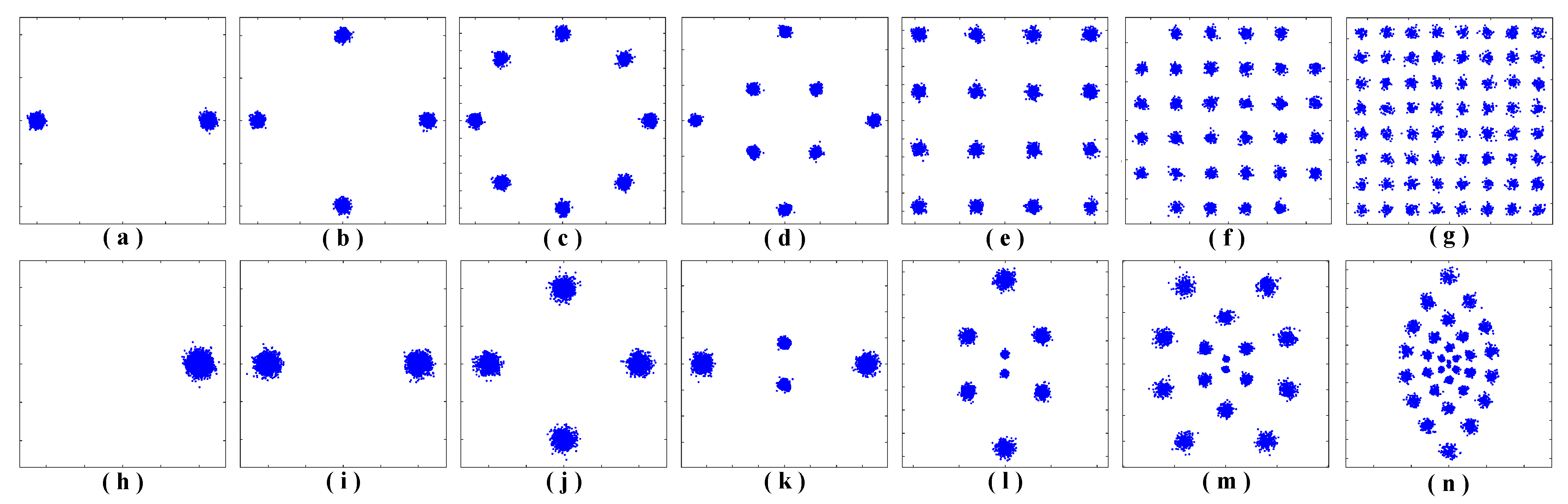
More intuitively, the changes between constellations before and after the square operation of these seven modulation formats (BPSK, QPSK, 8PSK and 8/16/32/64QAM) are shown in Figure 2. Using this property, it is easier to find the direction with the greatest variance, which will be useful in next step of principal axes correction.

Another property that should be noted is the average power after transformation. When considering the modulation format of BPSK in Equation (2), the average power of 1 is obtained according to $E_i^2=A_i^2·e^{j2\varphi }$, since $A_i=A_k=1$ and ${\theta }_i,{\theta }_k\in \{0,\pi \}$.

Focusing on Figure 2h, the average power of BPSK signals after the square operation is approximately 1, while others with an average power is approximately 0. Thus, the BPSK signals can be identified by detecting the average power after the square operation.

2.2. Principal Axes Correcting Based on PCA

Affected by the non-homogeneity of the laser sources at the transmitting end and receiving end, the overall phase rotation of the receiving constellation occurs. In the previous MFI methods based on constellation diagrams, constellation diagrams with different rotation angles need to be trained, which greatly increases the complexity of implementation. In this paper, principal axes correcting based on PCA is proposed to correct the constellations of different phase rotation angles to a unified datum. Thus, the phase rotation invariant properties to the constellation diagram are obtained without additional training on the phase rotation.

In contrast to the application of PCA in data dimension reduction, the usage of PCA in this paper is to find the direction with the greatest variance. Furthermore, the phase rotation is removed by correcting this direction. For convenience, the coordinate axis composed of the direction with the largest variance and one of its orthogonal vectors is called the principal axis.

As shown in Figure 2b–g, the distributions of the signals before the square operation are uniform, without any direction showing prominent variance. However, the distributions after the square operation exist in the desired directions, which is extracted and corrected through the process as follows.

For the received signals of length N after the square operation, a N $\times$ 2 matrix donated as $R$ is obtained:

$$R=\left[\begin{array}{cc}{r}_{11}& r_{12}\\ r_{21}& r_{22}\\ ⋮& ⋮\\ r_{N1}& r_{N2}\end{array}\right]=\left[\begin{array}{cc}\mathrm{Re}\left\{E_1^2\right\}& \mathrm{Im}\left\{E_1^2\right\}\\ \mathrm{Re}\left\{E_2^2\right\}& \mathrm{Im}\left\{E_2^2\right\}\\ ⋮& ⋮\\ \mathrm{Re}\left\{E_N^2\right\}& \mathrm{Im}\left\{E_N^2\right\}\end{array}\right]$$

(4)

where $\mathrm{Re}\{·\}$ and $\mathrm{Im}\{·\}$ means to take the real and imaginary parts of the signal, respectively. The values of real and imaginary parts are the projections of complex signals to the real axis (the magenta line Figure 3a) and imaginary axis (the red line in Figure 3a), respectively. It should be noted that here our signals suffer from phase rotation.

At first the mean values of $R$ is subtracted to obtain the zero-mean matrix $R_0$, and the element $r_{0,ij}$ in $R_0$ is calculated as follows:

$$r_{0,ij}=r_{ij}-\frac{1}{N}{\displaystyle \sum _{k=1}^N{r}_{kj}}$$

(5)

Next, the covariance matrix for the real and imaginary parts are calculated:

$$C=R_0{R}_0{}^T$$

(6)

The largest eigenvector of the covariance matrix points in the direction of the greatest variance and the second largest eigenvector is always orthogonal to the largest one. The principal axes as shown in Figure 3b can be attained by eigenvalue decomposition or singular value decomposition of the matrix.

The eigenvalue decomposition of covariance matrix can be expressed as:

$$C=U\mathsf{\Lambda }{U}^T$$

(7)

where $U=\left[\begin{array}{cc}{u}_1& u_2\end{array}\right]$ denotes the eigenvector matrix and $\mathsf{\Lambda }=diag({\lambda }_1,{\lambda }_2)$ is the diagonal matrix of eigenvalues. The eigenvectors $u_1$ and $u_2$ form the desired principal axes, which is shown in Figure 3b. The eigenvector with larger eigenvalue is the direction with the greatest variance (the red line in Figure 3b).

Looking further at Figure 2i–n, for original QPSK, 8PSK and 8QAM, the constellations after the square operation have the greatest variance in the real axis, and in the imaginary axis for 16/32/64QAM. Since the modulation formats of received signals are unknown during the MFI process, the direction with the greatest variance is corrected to the imaginary axis consistently. The direction with greatest variance is given by the following equation:

$$u=u_{\mathrm{m}}=\left[\begin{array}{c}{u}_x\\ u_y\end{array}\right],\mathrm{m}=\underset{i\in \{1,2\}}{\arg \max }{\lambda }_i$$

(8)

The angle $2\varphi$ of phase rotation after the square operation shown in Figure 3c is calculated as follows:

$$2\varphi =\{\begin{array}{ccc}\arccos (u_y)& ,& if{u}_x\ge 0\\ 2\pi -\arccos (u_y)& ,& if{u}_x<0\end{array}$$

(9)

Note that this angle is between the direction with the greatest variance and the imaginary axis, so it is $u_y$ instead of $u_x$ in the arc-cosine function.

Equation (3) shows that the phase rotation after the square operation is twice as much as before. Therefore, the angle of phase rotation before the square operation can be attained by halving the $2\varphi$.

Finally, the received data is projected onto the principal axes in Figure 3d to obtain the data without phase rotation as shown in Figure 3e.

In addition, the above method can also be applied to the BPSK signals without square operation, thus, restoring its phase.

After the principal axes correcting based on PCA, the signals without phase rotation is obtained, which is shown in Figure 4. Furthermore, according to the final MFI results, the constellations of QPSK and 8QAM can be rotated by 45 degrees, so as to realize the rough phase recovery of all modulated signals and reduce the complexity of the subsequent carrier phase recovery algorithm.

2.3. Density Distribution Analysis

Based on the signals like Figure 4, the density distribution analysis is employed to obtain the distribution of constellations.

Considering the signals are normalized to the average energy of 1, the maximum level of the in-phase component and quadrate component is approximately 1. Thus, a range for analysis is set, and any signal outside this range is treated as noise.

This range is then divided into several intervals, both in real and imaginary axes, and these intervals are used to divide a constellation into several blocks. The number of signals in each block is then calculated.

Finally, the density is calculated according to the number of signals in each block and then a matrix of density distribution is obtained.

2.4. Denoising and Smoothing Based on SVD

Since the received signal contains noise, there are many noise spots on the constellation diagram. To reduce the impact of noise on the accuracy of identification, the density matrix based on SVD is denoised, and the low-value zeroing method is used to highlight the main features.

The principle of it is to make use of the characteristic in which the large singular value of the density matrix contains the main information, while small singular values contain more noise. By SVD of the matrix, the part with large eigenvalues are extracted, and the denoised matrix is obtained.

For the density distribution matrix, $M$, SVD is applied:

$$M=US{V}^T$$

(10)

where $U$ and $V$ are the left and right singular matrices, respectively. $S$ is the singular value matrix of the following form:

$$S=diag({\sigma }_1,{\sigma }_2,\dots )$$

(11)

where ${\sigma }_i$ is the singular value. Selecting the first $n$ larger singular values, the density distribution matrix is reconstructed as:

$$M^{\prime }=U_{l\times n}{S}_{n\times n}{V}_{l\times n}{}^T=\left[\begin{array}{cccc}{m}_{11}& m_{12}& \cdots & m_{1l}\\ m_{21}& m_{22}& \cdots & m_{2l}\\ ⋮& ⋮& \ddots & ⋮\\ m_{l1}& m_{l2}& \cdots & m_{ll}\end{array}\right]$$

(12)

where $U_{{}_{l\times n}}$ and $V_{{}_{l\times n}}$ are the first $n$ columns of $U$ and $V$ with $l$ rows, respectively. $S_{n\times n}$ is the submatrix consisting of the first $n$ rows and the first $n$ columns of $S$.

After SVD, the density for blocks with low density is set to 0:

$$m_{jk}=\{\begin{array}{ccc}{m}_{jk}& ,& if{m}_{jk}\ge m_{thr}\\ 0& ,& if{m}_{jk}<m_{thr}\end{array}$$

(13)

Here, $m_{thr}$ is the threshold of low density.

2.5. SVM Classfication

Since BPSK was identified in the previous process, only the remaining modulation formats of QPSK, 8PSK and 8/16/32/64QAM need to be classified in the SVM classifier. In order to apply SVM classifier, the density distribution matrix is reshaped into a vector as the feature vector.

3. Simulation Setup and Results

A co-simulation platform is utilized to verify the proposed scheme. In the simulation system, the 28-GBaud signals of dual polarization (DP) BPSK, QPSK, 8PSK and 8/16/32/64QAM is transmitted through the fiber channel. The MFI accuracy is obtained after coherent reception and modulation format independent DSP processing.

3.1. Simulation Setup

The setup of the simulation system for the verification of the proposed blind MFI method is shown in Figure 5. First, pseudo-random bit sequences (PRBS) are generated and used to generate different modulation signals in the RF modulator at a symbol rate of 28-GBaud. In the polarization division multiplexing (PDM) IQ modulator, four channel RF signals are modulated to two optical carriers of different polarization states, respectively. The optical carriers are generated by a continuous-wave (CW) laser with a central wavelength of 1550 nm and linewidth of 10 kHz and are split into different polarization states by a polarization beam splitter (PBS). Then, the modulated optical signals in two polarization states are combined into one by using of polarization beam combiner (PBC). A combination of a tunable optical attenuator (VOA) and an erbium-doped fiber amplifier (EDFA) is used for the power control, and the optical power is set to 0 dBm before entering the transmission link. The transmission link consists of multiple loops, and each of them contain an 80 km standard single mode fiber (SSMF) and an EDFA whose gain is 16 dB to compensate for fiber attenuation. The attenuation, chromatic dispersion, differential group delay and nonlinear refractive index coefficient of SSMF are set as 0.2 dB/km, 16.75 ps/(nm∙km), 0.2 ps/km and 26 × 10⁻²¹ m²/W, respectively. The adjustment of different OSNR is achieved by coupling the amplified spontaneous emission (ASE) noise of different powers into the fiber at the receiving end using couplers. For this purpose, an EDFA is employed as an ASE noise source and a VOA is used to adjust the noise power. After the filtering out of out-of-band noise by an optical bandpass filter (OBPF) with a central wavelength of 1550 nm and bandwidth of 0.4 nm, the received signals are obtained in the DP coherent receiver. Finally, processed by the offline DSP in the figure, the modulation format information is obtained. It should be noted that the noise figure (NF) of the EDFA employed in the simulation system are all set as 4 dB.

3.2. Simulation Results

In the simulation system shown in Figure 5, OSNR varies from 5 dB to 35 dB with a step value of 1dB. In each OSNR, 1000 data sets are generated for each modulation format, and each of them contains 4096 samples of received signals. Then, the proposed MFI method is applied to the data sets to obtain the SVM classification feature sets. From each OSNR, 70% of the 1000 feature sets for each modulation format are mixed together as training features and the remaining 30% as testing features. Since features under different OSNR are mixed together for training and testing, the proposed method is blind and do not require prior information of OSNR.

In the process of proposed MFI, the average power of signals of each modulation format after square operation is shown in Figure 6. The lines of different modulation formats in Figure 6 represent the mean value of the average power of 1000 data sets under each OSNR and the regions in light-color represent the range of the average power of all data sets. As shown in Figure 6, BPSK is obviously different from other modulation formats in the average power after square operation, so the identification of BPSK can be realized only by setting a threshold value. In our work, the threshold shown by the dotted purple line is set to 0.0554.

After the square operation and average value detection of the signal power, principal axes correcting based on PCA is performed for the remaining signals. Take the 16QAM signals for example, the constellation before and after correcting are shown, respectively, in Figure 7a,b. The density distribution matrix is then obtained by the processing of density distribution analysis. For visualization and comparison, the distribution of the matrix is shown in Figure 7c. It can be seen that there are many noise points in the original matrix, which is not conducive to identification. In order to improve the identification accuracy, denoising and smoothing based on SVD is applied to the matrix. After the matrix is reconstructed with the first five largest eigenvalues, the distribution, as shown in Figure 7d, is obtained. By comparing these two matrices, it will be found that the density distribution of the matrix after our treatment is more concentrated and clearer.

Finally, the density distribution matrix is converted into the vector as the feature of the SVM classifier for training or testing, and the identification accuracy of the proposed MFI method is obtained as shown in Figure 8. The minimum OSNR values to achieve an identification accuracy of 100% for these seven modulation formats of BPSK, QPSK, 8PSK, 8/16/32/64QAM are 5 dB, 7 dB, 8 dB, 11 dB, 14 dB, 14 dB and 15 dB, respectively.

For the purpose of further evaluating the performance of the proposed MFI method, the minimum required OSNR for 100% identification accuracy has been compared with other methods found in [14,17,18,20,22,26]. The minimum OSNR required for the identification of modulation formats under different MFI methods is shown in Figure 9a, and the number of modulation formats identified by these methods is shown in Figure 9b.

For the identification of BPSK, QPSK, 8PSK and 64QAM, the minimum required OSNR for the proposed MFI method to achieve 100% accuracy are 5 dB, 7 dB, 8 dB and 15 dB, respectively. In other methods, the best achievable performance is 8 dB, 7.5 dB, 13 dB and 21 dB, respectively. Therefore, we achieved gains of OSNR of approximately 3 dB, 0.5 dB, 5 dB and 6 dB, respectively, in the identification of these modulation formats. For the remaining modulation formats of 8QAM, 16QAM and 32QAM, the minimum required OSNR for the proposed MFI are 11 dB, 14 dB and 14 dB, respectively, which is comparable to the best performance among other schemes. In terms of the number of identified modulation formats, the identification of most modulation formats is realized by the proposed method, with the total number of seven, while in other methods, they are four, four, six, six, four and four, respectively.

The more modulation formats an MFI method can identify, the more difficult it is to improve the accuracy because the increase in modulation formats means that more distinguishing features are required. However, as shown in Figure 9, the proposed method requires lower OSNR for the identification of most modulation formats, even though it needs to complete the identification of more modulation formats, which demonstrates the superior performance of the proposed method.

To evaluate the flexibility of the proposed method, the identification performance under different numbers of samples is tested. The average power after the square operation of different modulation formats with sample numbers of 2048, 1024 and 512 are shown in Figure 10a–c, respectively. As can be seen from these figures, there are still significant differences between BPSK and other modulation formats after the square operation, which means that BPSK can still be easily separated from other modulation formats. This can be reflected in the identification accuracy in Figure 10d–f: the identification accuracy of BPSK does not deteriorate with the decrease of the number of samples. Except for BPSK, the recognition performance of the other modulation formats decreases with the decrease in the number of samples.

For comparison, the minimum required OSNR values to achieve 100% identification accuracy for the proposed method and the other two methods in [14,18] under different sample numbers are shown in Figure 11. In this figure, the different colors of the bars represent a different number of samples. The horizontal axis is divided into seven equal parts according to the modulation formats, and under each modulation format the bars are grouped according to the MFI method. When the number of samples is 4096, the proposed method has obvious advantages in the identification of BPSK, QPSK, 8PSK and 16QAM, and achieved OSNR gains of at least 3 dB, 1 dB, 10 dB, 1 dB and 2 dB, respectively. Under the condition of 2048 samples, the best identification performances of BPSK, 8PSK, 16QAM and 64QAM are achieved by the proposed method, with the advantages of 3 dB, 12 dB, 4 dB and 6 dB. For BPSK and 8QAM, the same OSNR requirements for the best performances in the other methods are required for the proposed method. As for the sample number of 1024, the best performances are achieved by the proposed method for all modulation formats, and the OSNR requirements are reduced by at least 3 dB, 2 dB, 11 dB, 0 dB, 7 dB, 7 dB and 7 dB. It should be noted that the bars with slashes in Figure 11 indicates that 100% identification accuracy cannot be achieved until the corresponding OSNR (35 dB). When the number of samples is 512, only the comparison between the proposed method and the method in [14] is carried out. The results show that advantages in all modulation format identifications exist in the proposed scheme. For BPSK, QPSK, 8PSK, 16QAM and 64QAM, the advantages are 3 dB, 9 dB, 15 dB, 2 dB and 3 dB. These results show that our method works well even with reduced sample numbers, which is beneficial for low-complexity implementation.

4. Conclusions

In this work, a novel blind MFI method based on principal component analysis and singular value decomposition is proposed. Without any priori information, the proposed MFI can achieve accurate identification of seven modulation formats over a large OSNR range from 5 to 35 dB. In the proposed method, PCA is used to determine and correct the direction of the maximum variance of the received signals after square operation. Through this process, the effect of phase rotation can be removed and there is no need to train constellations under different rotations like the previous method based on constellation image processing, so the complexity of training is greatly reduced. The density distribution matrix instead of image is used to count the amplitude and phase information of the received signal constellation to prevent over-fitting caused by too many pixels in the image. SVD is employed to extract the main features of the density distribution matrix, and then the matrix is reconstructed by using the main features to achieve denoising and smoothing. Finally, a SVM classifier is used for the identification based on the matrix.

The performance of the proposed MFI method is evaluated in a 28-GBaud dual-polarization optical fiber communication system. Results shows that the minimum OSNR values required to achieve 100% accurate identification of BPSK, QPSK, 8PSK, 8QAM, 16QAM, 32QAM and 64QAM are 5 dB, 7 dB, 8 dB, 11 dB, 14 dB, 14 dB and 15 dB, respectively. Compared with the other six proposed methods, more types of modulation formats are identified in our method, with a total number of seven. More importantly, among these modulation formats, the best identification performance is achieved in our method, with the advantages up to 5 dB, 5 dB, 6 dB, 4 dB, 5.5 dB, 7.5 dB and 8dB. Additionally, in the identification of BPSK, QPSK, 8PSK and 8/16/32/64QAM, the OSNR gains of 5 dB, 5.04 dB, 9.38 dB, 6.14 dB, 4.75 dB, 8 dB and 9 dB relative to the 7% FEC threshold are obtained, respectively.

Furthermore, the influence of the number of samples on the performance is investigated. As the number of samples decreases, the accuracy of identification degrades. The results show that the proposed method still holds the advantage even under the number of samples of 4096, 2048, 1024 and 512, which is beneficial for low-complexity implementation.

For the further study, the challenge that needs to be faced is how to alleviate the influence on the phase caused by factors such as frequency offset and linewidth of laser source. After all, phase information has a prominent contribution in the identification of modulation formats, especially in the identification of multiple PSK modulation formats.

References

1. Naqvi, R.A.; Arsalan, M.; Rehman, A.; Rehman, A.U.; Loh, W.-K.; Paul, A. Deep Learning-Based Drivers Emotion Classification System in Time Series Data for Remote Applications. Remote Sens. 2020, 12, 587. [Google Scholar] [CrossRef] [Green Version]
2. Wang, F.; Yao, H.; Zhang, Q.; Wang, J.; Gao, R.; Guo, D.; Guizani, M. Dynamic Distributed Multi-Path Aided Load Balancing for Optical Data Center Networks. IEEE Trans. Netw. Serv. 2021, 15, 1. [Google Scholar] [CrossRef]
3. Jinno, M. Elastic Optical Networking: Roles and Benefits in Beyond 100-Gb/s Era. J. Lightwave Technol. 2017, 35, 1116–1124. [Google Scholar] [CrossRef]
4. Xiang, M.; Zhuge, Q.; Qiu, M.; Zhou, X.; Tang, M.; Liu, D.; Fu, S.; Plant, D.V. RF-Pilot Aided Modulation Format Identification for Hitless Coherent Transceiver. Opt. Express 2017, 25, 463. [Google Scholar] [CrossRef]
5. Lu, J.; Fu, S.; Deng, L.; Tang, M.; Hu, Z.; Liu, D.; Chan, C.-K. Blind and Fast Modulation Format Identification by Frequency-Offset Loading for Hitless Flexible Transceiver. In Proceedings of the Optical Fiber Communication Conference, OSA, San Diego, CA, USA, 11–15 March 2018; pp. 1–3. [Google Scholar]
6. Fu, S.; Xu, Z.; Lu, J.; Jiang, H.; Wu, Q.; Hu, Z.; Tang, M.; Liu, D.; Chan, C.C.-K. Modulation Format Identification Enabled by the Digital Frequency-Offset Loading Technique for Hitless Coherent Transceiver. Opt. Express 2018, 26, 7288. [Google Scholar] [CrossRef]
7. Isautier, P.; Mehta, K.; Stark, A.J.; Ralph, S.E. Robust Architecture for Autonomous Coherent Optical Receivers. J. Opt. Commun. Netw. 2015, 7, 864. [Google Scholar] [CrossRef]
8. Jiang, L.; Yan, L.; Yi, A.; Pan, Y.; Hao, M.; Pan, W.; Luo, B. An Effective Modulation Format Identification Based on Intensity Profile Features for Digital Coherent Receivers. J. Lightwave Technol. 2019, 37, 5067–5075. [Google Scholar] [CrossRef]
9. Zhao, Z.; Yang, A.; Guo, P. A Modulation Format Identification Method Based on Information Entropy Analysis of Received Optical Communication Signal. IEEE Access 2019, 7, 41492–41497. [Google Scholar] [CrossRef]
10. Cai, Q.; Guo, Y.; Li, P.; Bogris, A.; Shore, K.A.; Zhang, Y.; Wang, Y. Modulation Format Identification in Fiber Communications Using Single Dynamical Node-Based Photonic Reservoir Computing. Photon. Res. 2021, 9, B1–B8. [Google Scholar] [CrossRef]
11. Bilal, S.M.; Bosco, G.; Dong, Z.; Lau, A.P.T.; Lu, C. Blind Modulation Format Identification for Digital Coherent Receivers. Opt. Express 2015, 23, 26769. [Google Scholar] [CrossRef] [Green Version]
12. Lu, J.; Tan, Z.; Lau, A.P.T.; Fu, S.; Tang, M.; Lu, C. Modulation Format Identification Assisted by Sparse-Fast-Fourier-Transform for Hitless Flexible Coherent Transceivers. Opt. Express 2019, 27, 7072. [Google Scholar] [CrossRef] [PubMed]
13. Liu, G.; Proietti, R.; Zhang, K.; Lu, H.; Ben Yoo, S.J. Blind Modulation Format Identification Using Nonlinear Power Transformation. Opt. Express 2017, 25, 30895. [Google Scholar] [CrossRef] [PubMed]
14. Eltaieb, R.A.; Farghal, A.E.A.; Ahmed, H.H.; Saif, W.S.; Ragheb, A.; Alshebeili, S.A.; Shalaby, H.M.H.; Abd El-Samie, F.E. Efficient Classification of Optical Modulation Formats Based on Singular Value Decomposition and Radon Transformation. J. Lightwave Technol. 2020, 38, 619–631. [Google Scholar] [CrossRef]
15. Jiang, L.; Yan, L.; Yi, A.; Pan, Y.; Hao, M.; Pan, W.; Luo, B. Blind Optical Modulation Format Identification Assisted by Signal Intensity Fluctuation for Autonomous Digital Coherent Receivers. Opt. Express 2020, 28, 302. [Google Scholar] [CrossRef]
16. Yi, A.; Yan, L.; Jiang, L.; Pan, Y.; Luo, B.; Pan, W. Modulation Format Identification Based on Density Distributions in Stokes Plane for Digital Coherent Receivers. In Proceedings of the Asia Communications and Photonics Conference, Guangzhou, China, 10–13 November 2017; p. Su2A.29. [Google Scholar]
17. Jiang, L.; Yan, L.; Yi, A.; Pan, Y.; Bo, T.; Hao, M.; Pan, W.; Luo, B. Blind Density-Peak-Based Modulation Format Identification for Elastic Optical Networks. J. Lightwave Technol. 2018, 36, 2850–2858. [Google Scholar] [CrossRef]
18. Xu, H.; Yang, L.; Yu, X.; Zheng, Z.; Bai, C.; Sun, W.; Zhang, X. Blind and Low-Complexity Modulation Format Identification Scheme Using Principal Component Analysis of Stokes Parameters for Elastic Optical Networks. Opt. Express 2020, 28, 20249. [Google Scholar] [CrossRef]
19. Eltaieb, R.A.; Abouelela, H.A.E.; Saif, W.S.; Ragheb, A.; Farghal, A.E.A.; Ahmed, H.E.H.; Alshebeili, S.; Shalaby, H.M.H.; Abd El-Samie, F.E. Modulation Format Identification of Optical Signals: An Approach Based on Singular Value Decomposition of Stokes Space Projections. Appl. Opt. 2020, 59, 5989. [Google Scholar] [CrossRef]
20. Zhao, R.; Sun, W.; Xu, H.; Bai, C.; Tang, X.; Wang, Z.; Yang, L.; Cao, L.; Bi, Y.; Yu, X.; et al. Blind Modulation Format Identification Based on Improved PSO Clustering in a 2D Stokes Plane. Appl. Opt. 2021, 60, 9933. [Google Scholar] [CrossRef]
21. Khan, F.N.; Zhong, K.; Zhou, X.; Al-Arashi, W.H.; Yu, C.; Lu, C.; Lau, A.P.T. Joint OSNR Monitoring and Modulation Format Identification in Digital Coherent Receivers Using Deep Neural Networks. Opt. Express 2017, 25, 17767. [Google Scholar] [CrossRef]
22. Yi, A.; Yan, L.; Liu, H.; Jiang, L.; Pan, Y.; Luo, B.; Pan, W. Modulation Format Identification and OSNR Monitoring Using Density Distributions in Stokes Axes for Digital Coherent Receivers. Opt. Express 2019, 27, 4471. [Google Scholar] [CrossRef] [PubMed]
23. Zhang, W.; Zhu, D.; He, Z.; Zhang, N.; Zhang, X.; Zhang, H.; Li, Y. Identifying Modulation Formats through 2D Stokes Planes with Deep Neural Networks. Opt. Express 2018, 26, 23507. [Google Scholar] [CrossRef] [PubMed]
24. Wang, D.; Wang, M.; Zhang, M.; Zhang, Z.; Yang, H.; Li, J.; Li, J.; Chen, X. Cost-Effective and Data Size–Adaptive OPM at Intermediated Node Using Convolutional Neural Network-Based Image Processor. Opt. Express 2019, 27, 9403. [Google Scholar] [CrossRef]
25. Zhao, Y.; Yu, Z.; Wan, Z.; Hu, S.; Shu, L.; Zhang, J.; Xu, K. Low Complexity OSNR Monitoring and Modulation Format Identification Based on Binarized Neural Networks. J. Lightwave Technol. 2020, 38, 1314–1322. [Google Scholar] [CrossRef]
26. Cho, H.J.; Varughese, S.; Lippiatt, D.; Desalvo, R.; Tibuleac, S.; Ralph, S.E. Optical Performance Monitoring Using Digital Coherent Receivers and Convolutional Neural Networks. Opt. Express 2020, 28, 32087. [Google Scholar] [CrossRef] [PubMed]
27. Wan, Z.; Yu, Z.; Shu, L.; Zhao, Y.; Zhang, H.; Xu, K. Intelligent Optical Performance Monitor Using Multi-Task Learning Based Artificial Neural Network. Opt. Express 2019, 27, 11281. [Google Scholar] [CrossRef] [PubMed] [Green Version]
28. Cheng, Y.; Fu, S.; Tang, M.; Liu, D. Multi-Task Deep Neural Network (MT-DNN) Enabled Optical Performance Monitoring from Directly Detected PDM-QAM Signals. Opt. Express 2019, 27, 19062. [Google Scholar] [CrossRef]
29. Yu, Z.; Wan, Z.; Shu, L.; Hu, S.; Zhao, Y.; Zhang, J.; Xu, K. Loss Weight Adaptive Multi-Task Learning Based Optical Performance Monitor for Multiple Parameters Estimation. Opt. Express 2019, 27, 37041. [Google Scholar] [CrossRef]
30. Cheng, Y.; Zhang, W.; Fu, S.; Tang, M.; Liu, D. Transfer Learning Simplified Multi-Task Deep Neural Network for PDM-64QAM Optical Performance Monitoring. Opt. Express 2020, 28, 7607. [Google Scholar] [CrossRef]
31. Zhang, H.; Liu, P.; Guo, Y.; Zhang, L.; Huang, D. Blind Modulation Format Identification Using the DBSCAN Algorithm for Continuous-Variable Quantum Key Distribution. J. Opt. Soc. Am. B 2019, 36, B51–B58. [Google Scholar] [CrossRef]
32. Huang, L.; Xue, L.; Zhuge, Q.; Hu, W.; Yi, L. Modulation Format Identification under Stringent Bandwidth Limitation Based on an Artificial Neural Network. OSA Contin. 2021, 4, 96. [Google Scholar] [CrossRef]
33. Xiang, Q.; Yang, Y.; Zhang, Q.; Yao, Y. Joint, Accurate and Robust Optical Signal-to- Noise Ratio and Modulation Format Monitoring Scheme Using a Single Stokes-Parameter-Based Artificial Neural Network. Opt. Express 2021, 29, 7276. [Google Scholar] [CrossRef] [PubMed]
34. Mai, X.; Liu, J.; Wu, X.; Zhang, Q.; Guo, C.; Yang, Y.; Li, Z. Stokes Space Modulation Format Classification Based on Non-Iterative Clustering Algorithm for Coherent Optical Receivers. Opt. Express 2017, 25, 2038. [Google Scholar] [CrossRef] [PubMed]
Figure 1. The DSP flow in optical digital coherent receive; (a) Receiver DSP flow with MFI; (b) The proposed MFI method based on PCA and SVD.
Electronics 11 00612 g001
Figure 2. Constellation diagrams before and after the square operation of signals in modulation formats of BPSK, QPSK, 8PSK, 8QAM, 16QAM, 32QAM and 64QAM, respectively; (ag) Constellation diagrams before the square operation of signals; (hn) Constellation diagrams after the square operation of signals.
Electronics 11 00612 g002
Figure 3. The process diagram of principal axes corresponding based on PCA (64QAM for example). (a) The projections of signals on the real and imaginary axes after the square operation; (b) The principal axes formed by eigenvectors of covariance matrix; (c) The phase rotation of principal axes with respect to the original axes after the square operation; (d) The phase rotation of principal axes with respect to the original axes before the square operation; (e) Signals after principal axes correcting based on PCA.
Electronics 11 00612 g003
Figure 4. Signals after the principal axes correcting based on PCA. (ag) BPSK, QPSK, 8PSK and 8/16/32/64QAM, respectively.
Electronics 11 00612 g004
Figure 5. Simulation setup of the proposed blind MFI method.
Electronics 11 00612 g005
Figure 6. The average power of signals after the square operation.
Electronics 11 00612 g006
Figure 7. The process and effect of the proposed MFI method after the square operation, take the 16QAM signals for example. (a) Constellation before principal axes correcting; (b) Constellation after principal axes correcting; (c) Density matrix obtained by DDA; (d) Density distribution matrix after denoising and smoothing based on SVD.
Electronics 11 00612 g007
Figure 8. The identification accuracy of the proposed MFI.
Electronics 11 00612 g008
Figure 9. Performance comparison between the proposed method and the methods in the other literature, where * indicates that there is no identification result at the corresponding position. (a) The minimum required OSNR for 100% accurate identification; (b) Total number of identified modulation formats.
Electronics 11 00612 g009
Figure 10. The identification performance under a different number of samples. (ac) The average power of signals after square operation with the number of samples of 2048, 1024 and 512, respectively. (df) The identification accuracy under 2048, 1024 and 512 samples, respectively.
Electronics 11 00612 g010
Figure 11. The comparison of the minimum required OSNR to achieve 100% accuracy for different MFI methods, under a different number of samples.
Electronics 11 00612 g011
Publisher’s Note: MDPI stays neutral with regard to jurisdictional claims in published maps and institutional affiliations.