
Image Segmentation from Sparse Decomposition with a Pretrained Object-Detection Network


Abstract
:1. Introduction
- We designed a pretext task based on the sparse decomposition of object instances in videos for image segmentation. The task benefits from the sparsity of image instances and the inter-frame structure of videos;
- We propose an OLSeg model of three branches with bounding box prior. The location information of the object is obtained by a pretrained object-detection network. The model trained from videos is able to capture the foreground, background and segmentation mask in a single image;
- The proposed UnsupRL model is demonstrated to boost the performance effectively on various image segmentation benchmarks. The ablation study shows the gains of different components in OLSeg.
2. Related Work
2.1. Image Segmentation from Unlabeled Data
2.2. Pretrained Networks
2.3. Self-Supervised Learning
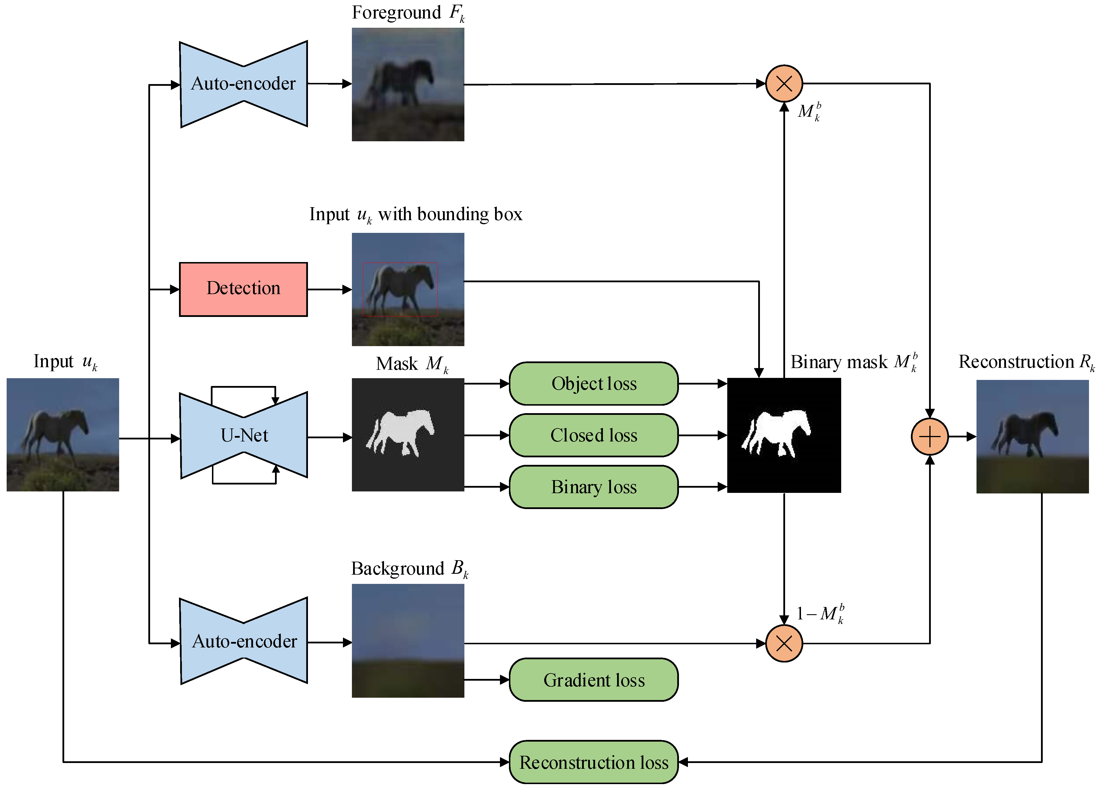
3. Object Location Segmentation (OLSeg)
3.1. The Foreground and Background Branches
| Algorithm 1: Training OLSeg. | |
| |
| 1: for to K do | |
| 2: | ▹ Foreground with the encoder channels |
| 3: | ▹ Background with the encoder channels |
| 4: | ▹ Segmentation mask |
| 5: | ▹ Area of the foreground object |
| 6: | ▹ Reconstruction image and binary mask |
| 7: end for | |
| 8: | ▹ Gradient loss |
| 9: | ▹ Object loss |
| 10: | ▹ Closed loss |
| 11: | ▹ Binary loss |
| 12: | ▹ Loss of the mask branch |
| 13: | ▹ Reconstruction loss |
| 14: | ▹ Overall loss of OLSeg |
| Output: Segmentation network . | |
3.2. The Mask Branch
3.3. The Overall Loss
4. Experiments
4.1. Implementation Details
4.1.1. Datasets
- The YouTube Objects dataset [51] is a large-scale dataset that includes 10 types of objects (e.g., airplane, bird, boat, car, cat, cow, dog, horse, motorbike, and train) downloaded from the YouTube website. It contains 5484 videos and a total of 571,089 video frames. The video consists of the object entering and leaving the line of sight, the object being occluded and the significant changes in the object scale and visual angle. The dataset provides ground-truth bounding boxes on the object of interest in one frame for each of 1407 video shots as the validation set.
- The Internet dataset [13] is a commonly used object segmentation dataset. There are 15,000 images downloaded from the internet. The dataset contains 4542 images of airplanes, 4347 images of cars and 6381 images of horses with the high-quality annotation masks.
- The Microsoft Research Cambridge (MSRC) dataset [52] contains 14 object classes and about 420 images with accurate pixel-wise labels. Each object in the dataset has different background, illumination and pose. This is a real-world dataset, which is often used to evaluate the image segmentation tasks.
4.1.2. Training Details
4.1.3. Evaluation Metrics
4.2. Parameter Selection
4.2.1. Encoder Output Channels in the Foreground and Background Branches
4.2.2. Hyperparameter for the Gradient Loss
4.2.3. Hyperparameter for the Object Loss
4.2.4. Hyperparameter for the Closed Loss
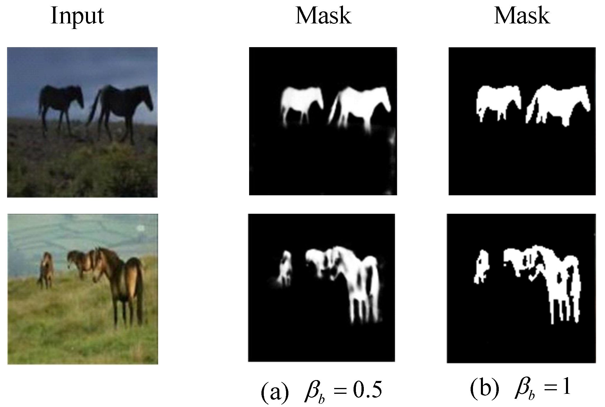
4.2.5. Hyperparameter for the Binary Loss
4.2.6. Results and Visualization
4.3. Evaluation on the Internet Dataset
4.4. Evaluation on the MSRC Dataset
4.5. Ablation Study
5. Conclusions
Author Contributions
Funding
Conflicts of Interest
References
- Kuutti, S.; Bowden, R.; Jin, Y.; Barber, P.; Fallah, S. A survey of deep learning applications to autonomous vehicle control. IEEE Trans. Intell. Transp. Syst. 2020, 22, 712–733. [Google Scholar] [CrossRef]
- Zhou, Z.; Siddiquee, M.M.R.; Tajbakhsh, N.; Liang, J. Unet++: Redesigning skip connections to exploit multiscale features in image segmentation. IEEE Trans. Med. Imaging 2019, 39, 1856–1867. [Google Scholar] [CrossRef] [PubMed] [Green Version]
- Lin, T.Y.; Maire, M.; Belongie, S.; Hays, J.; Perona, P.; Ramanan, D.; Dollár, P.; Zitnick, C.L. Microsoft coco: Common objects in context. In Proceedings of the European Conference on Computer Vision (ECCV), Zurich, Switzerland, 6–12 September 2014; Springe: Berlin/Heidelberg, Germany, 2014; pp. 740–755. [Google Scholar]
- Zhou, T.; Li, L.; Li, X.; Feng, C.M.; Li, J.; Shao, L. Group-wise learning for weakly supervised semantic segmentation. IEEE Trans. Image Process. 2021, 31, 799–811. [Google Scholar] [CrossRef] [PubMed]
- Wei, Y.; Xiao, H.; Shi, H.; Jie, Z.; Feng, J.; Huang, T.S. Revisiting dilated convolution: A simple approach for weakly-and semi-supervised semantic segmentation. In Proceedings of the IEEE Conference on Computer Vision and Pattern Recognition (CVPR), San Juan, PR, USA, 17–19 June 2018; pp. 7268–7277. [Google Scholar]
- Lee, J.; Kim, E.; Lee, S.; Lee, J.; Yoon, S. Ficklenet: Weakly and semi-supervised semantic image segmentation using stochastic inference. In Proceedings of the IEEE Conference on Computer Vision and Pattern Recognition (CVPR), Long Beach, CA, USA, 15–20 June 2019; pp. 5267–5276. [Google Scholar]
- Faktor, A.; Irani, M. Co-segmentation by composition. In Proceedings of the IEEE International Conference on Computer Vision (ICCV), Washington, DC, USA, 1–8 December 2013; pp. 1297–1304. [Google Scholar]
- Fan, J.; Zhang, Z.; Song, C.; Tan, T. Learning integral objects with intra-class discriminator for weakly-supervised semantic segmentation. In Proceedings of the IEEE Conference on Computer Vision and Pattern Recognition (CVPR), Kyoto, Japan, 13–19 June 2020; pp. 4283–4292. [Google Scholar]
- Hochbaum, D.S.; Singh, V. An efficient algorithm for co-segmentation. In Proceedings of the IEEE International Conference on Computer Vision (ICCV), Kyoto, Japan, 29 September–2 October 2009; pp. 269–276. [Google Scholar]
- Mukherjee, L.; Singh, V.; Dyer, C.R. Half-integrality based algorithms for cosegmentation of images. In Proceedings of the IEEE Conference on Computer Vision and Pattern Recognition (CVPR), Miami, FL, USA, 20–25 June 2009; pp. 2028–2035. [Google Scholar]
- Vicente, S.; Kolmogorov, V.; Rother, C. Cosegmentation revisited: Models and optimization. In Proceedings of the European Conference on Computer Vision (ECCV), Heraklion, Greece, 5–11 September 2010; Springer: Berlin/Heidelberg, Germany, 2010; pp. 465–479. [Google Scholar]
- Kim, G.; Xing, E.P.; Fei-Fei, L.; Kanade, T. Distributed cosegmentation via submodular optimization on anisotropic diffusion. In Proceedings of the IEEE International Conference on Computer Vision (ICCV), Barcelona, Spain, 6–13 November 2011; pp. 169–176. [Google Scholar]
- Rubinstein, M.; Joulin, A.; Kopf, J.; Liu, C. Unsupervised joint object discovery and segmentation in internet images. In Proceedings of the IEEE Conference on Computer Vision and Pattern Recognition (CVPR), Portland, OR, USA, 23–28 June 2013; pp. 1939–1946. [Google Scholar]
- Joulin, A.; Bach, F.; Ponce, J. Discriminative clustering for image co-segmentation. In Proceedings of the IEEE Conference on Computer Vision and Pattern Recognition (CVPR), San Francisco, CA, USA, 13–18 June 2010; pp. 1943–1950. [Google Scholar]
- Joulin, A.; Bach, F.; Ponce, J. Multi-class cosegmentation. In Proceedings of the IEEE Conference on Computer Vision and Pattern Recognition (CVPR), Providence, RI, USA, 16–21 June 2012; pp. 542–549. [Google Scholar]
- Quan, R.; Han, J.; Zhang, D.; Nie, F. Object co-segmentation via graph optimized-flexible manifold ranking. In Proceedings of the IEEE Conference on Computer Vision and Pattern Recognition (CVPR), Las Vegas, NV, USA, 27–30 June 2016; pp. 687–695. [Google Scholar]
- Zhao, D.; Ding, B.Q.; Wu, Y.L.; Chen, L.; Zhou, H.C. Unsupervised learning from videos for object discovery in single images. Symmetry 2021, 13, 38. [Google Scholar] [CrossRef]
- Hariharan, B.; Arbeláez, P.; Girshick, R.; Malik, J. Hypercolumns for object segmentation and fine-grained localization. In Proceedings of the IEEE Conference on Computer Vision and Pattern Recognition (CVPR), Boston, MA, USA, 7–12 June 2015; pp. 447–456. [Google Scholar]
- Zhou, B.; Khosla, A.; Lapedriza, A.; Oliva, A.; Torralba, A. Learning deep features for discriminative localization. In Proceedings of the IEEE Conference on Computer Vision and Pattern Recognition (CVPR), Las Vegas, NV, USA, 27–30 June 2016; pp. 2921–2929. [Google Scholar]
- Zhou, Z.H. Learnware: On the future of machine learning. Front. Comput. Sci. 2016, 10, 589–590. [Google Scholar] [CrossRef]
- Doersch, C.; Gupta, A.; Efros, A.A. Unsupervised visual representation learning by context prediction. In Proceedings of the IEEE International Conference on Computer Vision (ICCV), Santiago, Chile, 7–13 December 2015; pp. 1422–1430. [Google Scholar]
- Noroozi, M.; Favaro, P. Unsupervised learning of visual representations by solving jigsaw puzzles. In Proceedings of the European Conference on Computer Vision (ECCV), Amsterdam, The Netherlands, 11–14 October 2016; Springer: Berlin/Heidelberg, Germany, 2016; pp. 69–84. [Google Scholar]
- Larsson, G.; Maire, M.; Shakhnarovich, G. Learning representations for automatic colorization. In Proceedings of the European Conference on Computer Vision (ECCV), Amsterdam, The Netherlands, 11–14 October 2016; Springer: Berlin/Heidelberg, Germany, 2016; pp. 577–593. [Google Scholar]
- Pathak, D.; Girshick, R.; Dollár, P.; Darrell, T.; Hariharan, B. Learning features by watching objects move. In Proceedings of the IEEE Conference on Computer Vision and Pattern Recognition (CVPR), Honolulu, HI, USA, 21–26 July 2017; pp. 2701–2710. [Google Scholar]
- Mahendran, A.; Thewlis, J.; Vedaldi, A. Cross pixel optical-flow similarity for self-supervised learning. In Asian Conference on Computer Vision (ACCV); Springer: Berlin/Heidelberg, Germany, 2018; pp. 99–116. [Google Scholar]
- Dosovitskiy, A.; Springenberg, J.T.; Riedmiller, M.; Brox, T. Discriminative unsupervised feature learning with convolutional neural networks. Adv. Neural Inf. Process. Syst. 2014, 27, 766–774. [Google Scholar] [CrossRef] [PubMed] [Green Version]
- Radford, A.; Metz, L.; Chintala, S. Unsupervised representation learning with deep convolutional generative adversarial networks. arXiv 2015, arXiv:1511.06434. [Google Scholar]
- Rumelhart, D.E.; Hinton, G.E.; Williams, R.J. Learning representations by back-propagating errors. Nature 1986, 323, 533–536. [Google Scholar] [CrossRef]
- Ronneberger, O.; Fischer, P.; Brox, T. U-net: Convolutional networks for biomedical image segmentation. In International Conference on Medical Image Computing and Computer-Assisted Intervention (MICCAI); Springer: Berlin/Heidelberg, Germany, 2015; pp. 234–241. [Google Scholar]
- Bochkovskiy, A.; Wang, C.Y.; Liao, H.Y.M. Yolov4: Optimal speed and accuracy of object detection. arXiv 2020, arXiv:2004.10934. [Google Scholar]
- Batra, D.; Kowdle, A.; Parikh, D.; Luo, J.; Chen, T. icoseg: Interactive co-segmentation with intelligent scribble guidance. In Proceedings of the IEEE Conference on Computer Vision and Pattern Recognition (CVPR), San Francisco, CA, USA, 13–18 June 2010; pp. 3169–3176. [Google Scholar]
- Jerripothula, K.R.; Cai, J.; Yuan, J. Image co-segmentation via saliency co-fusion. IEEE Trans. Multimed. 2016, 18, 1896–1909. [Google Scholar] [CrossRef]
- Stretcu, O.; Leordeanu, M. Multiple frames matching for object discovery in video. In Proceedings of the British Machine Vision Conference (BMVC), Swansea, UK, 7–10 September 2015; Volume 1, p. 3. [Google Scholar]
- Papazoglou, A.; Ferrari, V. Fast object segmentation in unconstrained video. In Proceedings of the IEEE International Conference on Computer Vision (ICCV), Sydney, Australia, 1–8 December 2013; pp. 1777–1784. [Google Scholar]
- Koh, Y.J.; Jang, W.D.; Kim, C.S. POD: Discovering primary objects in videos based on evolutionary refinement of object recurrence, background, and primary object models. In Proceedings of the IEEE Conference on Computer Vision and Pattern Recognition (CVPR), Las Vegas, NV, USA, 27–30 June 2016; pp. 1068–1076. [Google Scholar]
- Wang, W.; Zhou, T.; Yu, F.; Dai, J.; Konukoglu, E.; Van Gool, L. Exploring cross-image pixel contrast for semantic segmentation. In Proceedings of the IEEE International Conference on Computer Vision (ICCV), Montreal, BC, Canada, 11–17 October 2021; pp. 7303–7313. [Google Scholar]
- Zhou, T.; Wang, S.; Zhou, Y.; Yao, Y.; Li, J.; Shao, L. Motion-attentive transition for zero-shot video object segmentation. In Proceedings of the AAAI Conference on Artificial Intelligence, New York, NY, USA, 7–12 February 2020; AAAI Press: Palo Alto, CA, USA, 2020; Volume 34, pp. 13066–13073. [Google Scholar]
- Rother, C.; Minka, T.; Blake, A.; Kolmogorov, V. Cosegmentation of image pairs by histogram matching-incorporating a global constraint into mrfs. In Proceedings of the IEEE Conference on Computer Vision and Pattern Recognition (CVPR), New York, NY, USA, 17–22 June 2006; Volume 1, pp. 993–1000. [Google Scholar]
- Liu, W.; Anguelov, D.; Erhan, D.; Szegedy, C.; Reed, S.; Fu, C.Y.; Berg, A.C. Ssd: Single shot multibox detector. In Proceedings of the European Conference on Computer Vision (ECCV), Amsterdam, The Netherlands, 11–14 October 2016; Springer: Berlin/Heidelberg, Germany, 2016; pp. 21–37. [Google Scholar]
- Zhao, H.; Shi, J.; Qi, X.; Wang, X.; Jia, J. Pyramid scene parsing network. In Proceedings of the IEEE Conference on Computer Vision and Pattern Recognition (CVPR), Honolulu, HI, USA, 21–26 July 2017; pp. 2881–2890. [Google Scholar]
- Mahajan, D.; Girshick, R.; Ramanathan, V.; He, K.; Paluri, M.; Li, Y.; Bharambe, A.; Van Der Maaten, L. Exploring the limits of weakly supervised pretraining. In Proceedings of the European Conference on Computer Vision (ECCV), Munich, Germany, 8–14 September 2018; pp. 181–196. [Google Scholar]
- Wei, X.S.; Luo, J.H.; Wu, J.; Zhou, Z.H. Selective convolutional descriptor aggregation for fine-grained image retrieval. IEEE Trans. Image Process. 2017, 26, 2868–2881. [Google Scholar] [CrossRef] [PubMed] [Green Version]
- Vincent, P.; Larochelle, H.; Bengio, Y.; Manzagol, P.A. Extracting and composing robust features with denoising autoencoders. In Proceedings of the International Conference on Machine Learning (ICML), Helsinki, Finland, 5–9 July 2008; pp. 1096–1103. [Google Scholar]
- Le, Q.V. Building high-level features using large scale unsupervised learning. In Proceedings of the International Conference on Acoustics, Speech and Signal Processing (ICASSP), Vancouver, BC, Canada, 26–31 May 2013; pp. 8595–8598. [Google Scholar]
- Goodfellow, I.; Pouget-Abadie, J.; Mirza, M.; Xu, B.; Warde-Farley, D.; Ozair, S.; Courville, A.; Bengio, Y. Generative adversarial nets. arXiv 2014, arXiv:1406.2661. [Google Scholar]
- Pathak, D.; Krahenbuhl, P.; Donahue, J.; Darrell, T.; Efros, A.A. Context encoders: Feature learning by inpainting. In Proceedings of the IEEE Conference on Computer Vision and Pattern Recognition (CVPR), Las Vegas, NV, USA, 27–30 June 2016; pp. 2536–2544. [Google Scholar]
- Noroozi, M.; Pirsiavash, H.; Favaro, P. Representation learning by learning to count. In Proceedings of the IEEE International Conference on Computer Vision (ICCV), Venice, Italy, 22–29 October 2017; pp. 5898–5906. [Google Scholar]
- Gidaris, S.; Singh, P.; Komodakis, N. Unsupervised representation learning by predicting image rotations. arXiv 2018, arXiv:1803.07728. [Google Scholar]
- Lee, H.Y.; Huang, J.B.; Singh, M.; Yang, M.H. Unsupervised representation learning by sorting sequences. In Proceedings of the IEEE International Conference on Computer Vision (ICCV), Venice, Italy, 22–29 October 2017; pp. 667–676. [Google Scholar]
- Wei, D.; Lim, J.J.; Zisserman, A.; Freeman, W.T. Learning and using the arrow of time. In Proceedings of the IEEE Conference on Computer Vision and Pattern Recognition (CVPR), Salt Lake City, UT, USA, 18–23 June 2018; pp. 8052–8060. [Google Scholar]
- Prest, A.; Leistner, C.; Civera, J.; Schmid, C.; Ferrari, V. Learning object class detectors from weakly annotated video. In Proceedings of the IEEE Conference on Computer Vision and Pattern Recognition (CVPR), Providence, RI, USA, 16–21 June 2012; pp. 3282–3289. [Google Scholar]
- Shotton, J.; Winn, J.; Rother, C.; Criminisi, A. Textonboost: Joint appearance, shape and context modeling for multi-class object recognition and segmentation. In Proceedings of the European Conference on Computer Vision (ECCV), Amsterdam, The Netherlands, 11–14 October 2016; Springer: Berlin/Heidelberg, Germany, 2006; pp. 1–15. [Google Scholar]
- He, K.; Zhang, X.; Ren, S.; Sun, J. Deep residual learning for image recognition. In Proceedings of the IEEE Conference on Computer Vision and Pattern Recognition (CVPR), Las Vegas, NV, USA, 27–30 June 2016; pp. 770–778. [Google Scholar]
- Odena, A.; Dumoulin, V.; Olah, C. Deconvolution and checkerboard artifacts. Distill 2016, 1, e3. [Google Scholar] [CrossRef]


| Parameters | Values |
|---|---|
| Size of input | 128 × 128 |
| Size of output | 128 × 128 |
| Optimizer | Adam |
| Learning rate | 0.00001 |
| Epochs | 10 |
| Batch size | 16 |
| Output channels of encoder in the foreground branch | 128 |
| Output channels of encoder in the background branch | 32 |
| Hyperparameter | 1.5 |
| Hyperparameter | 0.15 |
| Hyperparameter | 0.05 |
| Hyperparameter | 1 |
| Methods | Airplane | Bird | Boat | Car | Cat | Cow | Dog | Horse | Mbike | Train | Avg | Time (s) |
|---|---|---|---|---|---|---|---|---|---|---|---|---|
| Stretcu et al. [33] | 38.3 | 62.5 | 51.1 | 54.9 | 64.3 | 52.9 | 44.3 | 43.8 | 41.9 | 45.8 | 49.9 | 6.9 |
| Papazoglou et al. [34] | 65.4 | 67.3 | 38.9 | 65.2 | 46.3 | 40.2 | 65.3 | 48.4 | 39.0 | 25.0 | 50.1 | 4 |
| Koh et al. [35] | 64.3 | 63.2 | 73.3 | 68.9 | 44.4 | 62.5 | 71.4 | 52.3 | 78.6 | 23.1 | 60.2 | N/A |
| OLSeg | 70.9 | 60.8 | 74.7 | 61.3 | 65.5 | 64.1 | 66.3 | 56.7 | 45.1 | 48.3 | 61.4 | 0.03 |
| Methods | Airplane | Car | Horse | |||
|---|---|---|---|---|---|---|
| Joulin et al. [14] | 49.25 | 15.36 | 58.70 | 37.15 | 63.84 | 30.16 |
| Joulin et al. [15] | 47.48 | 11.72 | 59.20 | 35.15 | 64.22 | 29.53 |
| Kim et al. [12] | 80.20 | 7.90 | 68.85 | 0.04 | 75.12 | 6.43 |
| Rubinstein et al. [13] | 88.04 | 55.81 | 85.38 | 64.42 | 82.81 | 51.65 |
| Quan et al. [16] | 91.00 | 56.30 | 88.50 | 66.80 | 89.30 | 58.10 |
| OLSeg | 91.87 | 61.50 | 90.23 | 68.45 | 89.56 | 58.72 |
| MSRC | Joulin et al. [14] | Joulin et al. [15] | Kim et al. [12] | Rubinstein et al. [13] | Quan et al. [16] | OLSeg |
|---|---|---|---|---|---|---|
| 71.53 | 77.01 | 61.34 | 78.31 | 86.21 | 87.56 | |
| 45.27 | 50.97 | 34.48 | 56.69 | 63.32 | 65.85 |
| Methods | Internet | MSRC | ||
|---|---|---|---|---|
| OLSeg | 90.55 | 62.89 | 87.56 | 65.85 |
| Without the gradient loss | 83.12 | 54.67 | 78.73 | 56.29 |
| Without the closed loss | 84.62 | 56.02 | 80.84 | 58.23 |
| Without the binary loss | 86.45 | 59.13 | 84.01 | 62.72 |
Publisher’s Note: MDPI stays neutral with regard to jurisdictional claims in published maps and institutional affiliations. |
© 2022 by the authors. Licensee MDPI, Basel, Switzerland. This article is an open access article distributed under the terms and conditions of the Creative Commons Attribution (CC BY) license (https://creativecommons.org/licenses/by/4.0/).
Share and Cite
Wu, Y.; Lv, C.; Ding, B.; Chen, L.; Zhou, B.; Zhou, H. Image Segmentation from Sparse Decomposition with a Pretrained Object-Detection Network. Electronics 2022, 11, 639. https://doi.org/10.3390/electronics11040639
Wu Y, Lv C, Ding B, Chen L, Zhou B, Zhou H. Image Segmentation from Sparse Decomposition with a Pretrained Object-Detection Network. Electronics. 2022; 11(4):639. https://doi.org/10.3390/electronics11040639
Chicago/Turabian StyleWu, Yulin, Chuandong Lv, Baoqing Ding, Lei Chen, Bin Zhou, and Hongchao Zhou. 2022. "Image Segmentation from Sparse Decomposition with a Pretrained Object-Detection Network" Electronics 11, no. 4: 639. https://doi.org/10.3390/electronics11040639
APA StyleWu, Y., Lv, C., Ding, B., Chen, L., Zhou, B., & Zhou, H. (2022). Image Segmentation from Sparse Decomposition with a Pretrained Object-Detection Network. Electronics, 11(4), 639. https://doi.org/10.3390/electronics11040639