1. Introduction
Radio frequency spectrum monitoring is a major issue in communications applications due to the expansion of wireless technologies which implies a reduction of available band spectrum. For example, the Internet-of-Things (IoT) communication has recently emerged in many applications such as Smart City which has the advantage of low power consumption. The number of IoT connected devices will explode in the near future. Consequently, a specific bandwidth will be saturated because several wireless devices will be connected at the same time. It is possible to handle this problem by using cognitive radios which are able to manage dynamically the spectrum. During many years, spectrum monitoring has been based on the Shannon–Nyquist sampling theorem [
1,
2]. Indeed, it is possible to reconstruct a signal by picking samples at periodic time. Mathematically, the Nyquist rate
is determined for a band-limited spectrum
by
[
3]. However, in practice, this method is difficult to use in a wideband context, typically more than 1 GHz. Indeed, Nyquist frequency can exceed the specifications of existing Analog to Digital Converters (ADC) and sampling at a high rate introduces amount of data which requires a huge storage capacity.
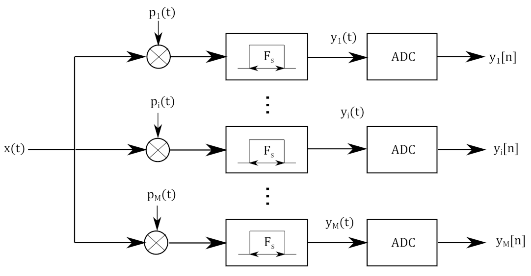
Several techniques, depending or not on the knowledge of the carrier frequency, have been developed to monitor a multiband spectrum (random demodulator [
4,
5], multicoset sampling [
6,
7], Modulated Wideband Converter [
8], quadrature analog-to-information converter [
9], time-segmented quadrature analog-to-information converter [
10], random triggering based modulated wideband compressive sampling [
11] and non uniform wavelet sampling [
12,
13]). In the case of known carrier frequencies, a band of interest is firstly chosen and the signal is demodulated by its carrier frequency. Unwanted bands of signals were rejected by a low-pass filter. Finally, the selected band is sampled by an ADC at a realistic rate [
14]. In the case of unknown carrier frequencies, it is a hard challenge to blindly recover a signal from the measured samples.
One major problem to monitor wideband signal is to choose appropriate ADCs. An ADC is first characterized by a track and hold circuit which tracks the value of the analog input signal and holds it at a constant value between clock cycles. This analog value is then digitized by a quantization module. Therefore, an ADC is generally characterized by an input bandwidth
B corresponding to the maximal frequency supported by the Track/Hold module and by a sampling frequency
equal to the inverse of the time duration
of the quantization processing. Indeed, an ADC can be limited for two main reasons. Firstly, its bandwidth
B needs to be equal to the bandwidth of the signal input, which can be huge in practice. Moreover, according to the Shannon–Nyquist sampling theorem, its sampling frequency
could be very high, which can not be provided by actual ADCs. The first issue can be addressed by multi channel sampling schemes. Uniform interleaved sampling [
15] can be used to sample a wideband signal. Assume that a wideband signal
needs to be sampled at a Nyquist frequency
M times higher than the frequency
specified by an ADC. Instead of using a single ADC at a high rate, a solution is to use
M ADCs in parallel and interleave them with delays. By choosing delays spaced of
, with
,
M samples are contained in the periodic time
. If samples are multiplexed, the scheme can be seen as an unique ADC with a sampling frequency
. To respect the Shannon–Nyquist theorem, i.e.,
, it is necessary to fix the ADC sampling frequency
. Consequently, the sampling frequency is reduced by a factor
M. Although this approach solves the problem of limitation of the ADC sampling frequency
, it still requires an ADC with bandwidth
B at least equal to the input signal bandwidth. Moreover, maintaining constant time shifts of the order of
is difficult to implement [
8]. Nonuniform interleaved sampling [
16] has also been proposed to sample multiband signals. Compared to the uniform interleaved sampling, delays are irregularly spaced. However, to implement this algorithm, delays are assumed periodic. As in the uniform case, the nonuniform sampling allows the ADC frequency
to be reduced by a factor
M; however, it is still also limited because the ADC bandwidth
B must be equal to the bandwidth of the input signal. This approach has the advantage of being compressive. However, this method is difficult to use in practice due to the performance of the ADCs.
Recently, a new approach has been proposed allowing sampling at sub-Nyquist rate. This approach is called compressed sensing, or more generally compressive sampling. Compressed sensing has recently emerged as a potential framework for signal acquisition in many applications [
17], especially to monitor a wideband spectrum [
18]. In [
19,
20], the authors showed that a finite-dimensional signal which has a sparse representation in some basis can be recovered from a small set of linear measurements. Theoretical aspects of compressed sensing have been largely addressed in the literature. For instance, many studies on the design of the measurements scheme have been proposed as in [
21,
22]. However, few works have considered practical constraints of compressed sensing. Indeed, the design of the measurements schemes and their application to practical acquisition systems such as spectrum sensing systems remain a central challenge in the field of compressed sensing. More recently, the authors in [
8] proposed a new scheme, called Modulated Wideband Converter (MWC), which allows sampling at rates much lower than the Nyquist rate while considering practical implementation issues of compressed sensing. In this work, the band locations are unknown to the user. Generally, the proposed scheme architecture in [
8] can be decomposed into two main steps. Firstly, an analog processing is applied to the input signal in order to create several channels through modulation and filtering. In the second step, each channel is sampled by ADCs.
In this paper, the MWC scheme proposed in [
8] is considered which, to the best of our knowledge, seems to be the most convenient scheme in terms of recovering performance, complexity and practical implementation. Some practical implementations of compressed sensing systems have been already proposed [
4,
23,
24]. To realize a prototype of compressed sensing based on MWC scheme, three solutions can be followed. The first solution is to use commercial off-the-shelf components. However, this type of solution had a significant risk in terms of development due to the deflects introduced by all components. The second solution would be to develop a custom silicium solution [
24]. However, this solution can be very expensive and dicey for testing and debugging steps. The third (chosen solution) solution is to design an analog board with discrete components to achieve this functionality. Some authors have already addressed the design of MWC system and a non-exhaustive list of references is given here [
23,
25,
26,
27,
28,
29]. Our analog board has a number of physical channels
M limited to four channels and the length of the modulating sequences
L is realistic and set to 96. These parameters will be explained in detail in
Section 2.
One important step in compressed sensing framework is the knowledge of the sensing matrix required for the reconstruction step. In the ideal case, the sensing matrix can be perfectly estimated from modulating waveforms. However, in practice, some problems introduced by analog components (such as nonlinearities of mixers, phase/attenuation/selectivity of lowpass filters, desynchronization between modulating waveforms) have been identified by researchers from Technion—Israël Institute of Technology [
23]. The authors have proposed a calibration method to estimate the sensing matrix. They estimate one column of the sensing matrix by injecting sine function at a specific frequency. This step is repeated by changing the frequency until all columns of the sensing matrix are estimated. This technique can be considered as a reference. Some researchers have exploited this work to propose calibration algorithms [
29,
30,
31,
32,
33] based on the measurements of different single tones. In our opinion, one drawback of this procedure is that this task can be time consuming and annoying when the number of columns of the sensing matrix
L is high because the same step must be repeated many times. Consequently, the motivation of this paper is to develop a new MWC hardware calibration technique from only one measurement. The idea has been already proposed in [
34,
35] where the calibration signal is a mixture of single tones.
Table 1 sums up the difference between our MWC calibration method and other MWC calibration methods.
The main contributions of this paper are:
A prototype of compressed sensing based on MWC scheme has been developed to monitor a wideband spectrum at Nyquist frequency GHz. The prototype has physical channels. The total equivalent sampling rate is equal to MHz which is 29.16% of the Nyquist rate.
The calibration signal is a white noise signal. Compared to methods based on iterative single-tones or mixture of single-tone signals, our new calibration method has the advantage of being more practical in terms of simplicity of implementation and time saving because only one measurement is used to complete the calibration. The calibration signal spectrum is totally flat in the band of interest and covers all the bandwidths of the spectrum to analyze.
The calibration method uses an advanced resynchronization preprocessing. Our calibration method offers slightly better spectrum reconstruction performances compared to reference method [
23].
The remainder of this paper is organized as follows:
Section 2 describes the MWC theoretical background.
Section 3 presents our prototype of compressed sensing based on MWC scheme.
Section 4 presents our calibration method.
Section 5 presents spectrum reconstruction performances and examples of spectrum reconstruction obtained with our calibration method from MWC output.
3. MWC Hardware Prototype
The genesis of this work, which is a part of a large innovative project dedicated to coastal surveillance, is to monitor a wideband spectrum at Nyquist frequency
GHz. To the best of our knowledge, the MWC seems to be the most convenient scheme in terms of recovering performance, complexity and practical implementation. Some prototypes [
23,
25,
28] of compressed sampling scheme based on MWC with different parameters have been already developed. For simplicity of implementation, the number of physical channels
M must be realistic as in [
23,
25,
28]. For simplicity of generation, the length of mixing sequences
L has been chosen lower than the length of mixing sequences used in [
23,
25,
28]. The values of these parameters are given in
Section 3.1.
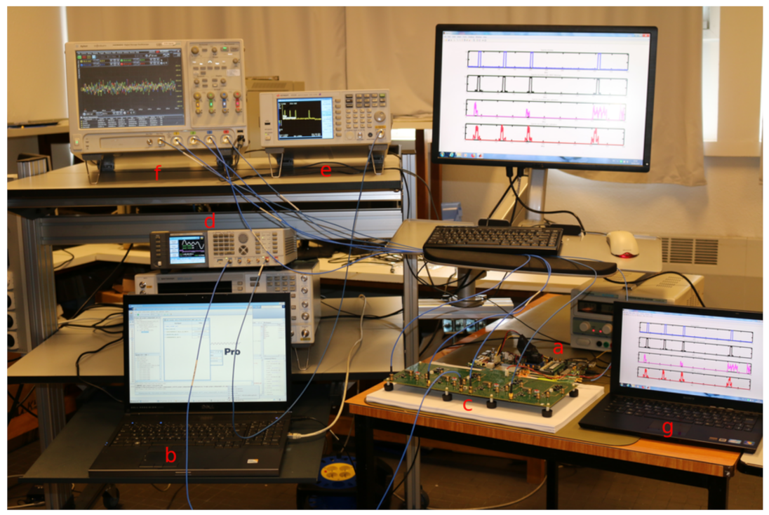
Figure 3 shows our prototype of compressed sampling scheme based on MWC.
In this section, we motivate the choice of the prototype parameters and we present the analog board. An example of spectrum reconstruction without calibration is directly processed from data acquired by the prototype.
3.1. Prototype Parameters
The Nyquist frequency is set to GHz. The number of physical channels is set to in order to save hardware size and price. Pseudo-random binary signal have been chosen for simplicity of generation for the mixing sequences which length is fixed . In our scenario, the bandwidth of each transmitter is set to . To choice the collapsing factor, a trade-off between reasonable total equivalent sampling rate and maximal number of symmetric transmitters must be conducted. Related to the model, the input bandwidth is divided into L subbands with a bandwidth . With this choice, each transmitter can be positioned inside one channel of the MWC or it can be astride at most two channels. The worst case should be taken into account, namely, that each transmitter can locate astride two channels of the equivalent model. We choose a collapsing factor . The condition of sparsity must be verified such as where is the maximum number of active channels in the MWC equivalent model. The number of active channels in the MWC equivalent model is strictly set and to take into account the worst case that the transmitters can be astride two active channels, then we set . Since the transmitters are symmetric in real case; then, we finally set the maximum number of transmitters , which leads to . The bandwith of ideal low-pass filter and ADC (and the sampling rate) is equal to MHz, which involves a cut-off frequency MHz. The repetition frequency of modulating waveforms is equal to MHz. The bandwidth of each transmitter is fixed to MHz. The total equivalent sampling rate is equal to MHz which is 29.16 % of the Nyquist rate.
For the rest of the paper, input signal has transmitters which corresponds to the occupancy of 4 subbands which are symmetric, equivalent to occupy subbands in Nyquist bandwidth.
Table 2 sums up the parameters of the MWC.
The relation between the Signal to Noise ratio (SNR) in the transmitting subbands and the Signal to Noise ratio in the whole spectrum is computed by:
3.2. Analog Board
A (Avnet) “ML605 DSP Kit with AD/DA board” embedding a (Xilinx) Virtex-6 FPGA is used to generate pseudo-random modulating waveforms. The Gigabit-Transceiver X (GTX) high-speed SERDES (SERializer-DESrializer) transceivers embedded in its (Xilinx) LX240T Virtex-6 FPGA model and the different debugging cores from (Xilinx) Chipscope Pro for the Virtex-6 FPGA gave us the required programmability, speed and development flexibility to output the differential signals implementing the mixing sequences. This allowed us to dynamically choose (per channel) the sequence from a compiled list, fix its size, turn on and off channels, adjust output amplitudes and add some pre-emphasis or post-emphasis effects to signals. With recompilation, we can also add new sequences to the list and change the bit rate. The clock source can be physically changed to appropriate external generators. GTXs 0, 1, 2 and 3 are, respectively, connected to channels 1, 2, 3 and 4 of a MWC analog frond-end board.
A Keysight 81180A arbitrary waveform generator is used to generate the input signal. The channel 1 is plugged to a Keysight N9320B spectrum analyzer (range frequency 9 kHz to 3 GHz) to control the simulated input signal and the channel 2 is plugged to a SCA-4-10+ splitter from Mini-Circuits
® of the MWC analog front-end board with four channels. Each channel has one M1-0008 mixer from MArki
® and one SXLP-36+ low-pass filter from Mini-Circuits
® with a cut-off frequency
MHz. The SXLP-36+ filter has been chosen to match the design of the ideal low-pass filter (sharp cut-off, flat band in frequency range [DC-36] MHz).
Figure 4 shows a block diagram of the analog board.
A PC controls the generation of the modulating waveforms with the ML605 board and also the generation of the input signal with the arbitrary waveform generator.
Output signals are acquired and saved by a DSO90404A Agilent Infiniium four-channel scope which provides up 8 GHz real-time bandwidth and 40 Gsample/s sample rate. The outputs are acquired at 40 Gsample/s. To be able to synchronize the acquisition with respect to the modulating waveforms, an extra signal equivalent to a pulse is also generated by the GTX 7 of ML605 board which is plugged to the scope external trigger.
Figure 5 shows our compressed sampling prototype analog front-end board and the ML605 control board.
A PC is used to apply a post-processing for the reconstruction. MWC outputs are downsampled at MHz. Then a digital filter with a bandwidth is applied to eliminate aliasing effect and filtered outputs are downsampled at .
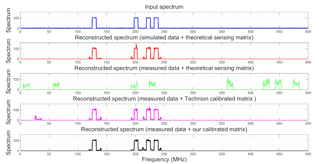
3.3. Example of Reconstruction without Calibration
Figure 6 shows an example of spectrum reconstruction without calibration at
dB from the theoretical sensing matrix. Each reconstructed spectrum is in linear scale and has been normalized such that the power of each reconstructed spectrum is equal to the power of the input spectrum. Real data have been acquired and saved by the scope. Spectrum reconstruction of measured data with the theoretical sensing matrix (calculated directly from modulating waveforms) have bad detection performances and high false alarm compared to the results obtained for the simulated data. This result is due to incorrect estimation of the sensing matrix linked to analog components. Indeed, analog components introduce phases which change the theoretical sensing matrix. Consequently, the goal of the next section is to present a new calibration method to estimate sensing matrix coefficients.
4. Proposed Calibration Method
To ensure correct spectrum recovery, the major problem is to estimate precisely the sensing matrix . In ideal case, it is possible to compute the sensing matrix by knowing the modulating waveforms. However, in practice, this process brings bad results due to the hardware design such as nonlinearities of mixers and amplifiers, filters deflects, desynchronization of modulating waveforms, connectors and cables. Consequently, a calibration method must be used to estimate sensing matrix coefficients.
In 2014, a calibration method for MWC system, developed by Technion, has been proposed in [
23] and provides good reconstruction performance for SNR in the whole spectrum greater than 8 dB. The process estimates the system’s response for every frequency band by injecting consecutive sinusoidal inputs at incremental rates. By knowing the sine frequency of input signal and MWC outputs, it is possible to identify one column of the sensing matrix. This step must be repeated with sine functions at different frequencies to estimate all columns of the sensing matrix. From our experience it appears that this process can be long and difficult because the same step must be repeated for all columns. For our system configuration with 96 columns, the process should be repeated 49 times to complete the calibration (due to symmetries, some columns can be estimated by pairs). That is the reason why we propose a new calibration method which estimates the sensing matrix
by injecting a single white noise signal.
Note that the calibration developed by Technion can be considered as a reference. Indeed, researchers who design the MWC system come also from Technion. For the rest of the paper, our results will be compared with those obtained with calibration technique developed by Technion.
4.1. Calibration Algorithm
The calibration algorithm is divided into two main steps: preprocessing resynchronization step and sensing matrix estimation step.
A specific white noise signal, called “calibration signal”, is first generated (
Figure 7). This signal is periodic with the period equal to the size of the block used for the reconstruction. Its basic pattern (
N samples at
) is first generated in the Fourier domain, specifying perfectly flat amplitudes and random phases, then an inverse-Fast Fourier Transform (FFT) provides the samples in the time domain.
After injection of input signal, the outputs of MWC system are recorded. In parallel, we also record a pulse wave (output of GTX 7) which identifies the beginning of modulating waveforms.
4.1.1. Resynchronization Preprocessing Step
The resynchronization preprocessing step estimates the optimal shift value which minimizes the Frobenius norm (or maximizes the inverse Frobenius norm) of the residual matrix between shifted version of output signal and reconstructed output (relative to the equivalent model) knowing the input signal.
To complete the calibration, we must synchronize three signals:
In practice, it is possible to synchronize together only two signals (for example, the outputs and the pulse wave which identifies the modulating waveforms starts), but not three signals. To achieve this task, digital processing must be followed.
Figure 8 illustrates the synchronization method. At the beginning of the process, we know:
Firstly, a coarse synchronization is conducted to determine the starting sample value
corresponding of the beginning of the input pattern. Let us note
the number of samples in an output block (corresponding to an input block of
N samples). Output blocks, shifted by
samples from the beginning of recorded output
, noted
, are formed to be able to estimate
. By knowing
, which is the vector
z restricted to its active components, with Equation (
3), and using the pseudo-inverse with Equation (
4), the sensing matrix
can be estimated by:
Then, the reconstructed signal
relative to the equivalent model knowing the input signal is computed by:
is obtained by minimizing the Frobenius norm on the residual matrix
:
with
the Frobenius norm.
For example,
is equal to 2041 in
Figure 9. Note that for easier visualization it is the inverse of the Frobenius norm (with respect to
d) which is shown on the figure.
Since, as previously mentioned, we computed it for
, we have two peaks on
Figure 9, while computation could be restricted to
, this extension is preferred, in order to confirm visually (by the presence of two similar peaks separated by
samples) the validity of the obtained synchronization.
A fine synchronization (see
Figure 10) is then performed. Small corrections
are applied to
and evaluated using the same procedure as described above, that is using Equation (
7), Equation (
8) and Equation (
9). The samples required for this fine synchronization are obtained by oversampling the outputs by a factor 32. The computational load remains small because we have to test only a few values of
.
Now, we know that the first output block corresponding to an input pattern starts at
samples from the beginning. This is represented by “input synchro” in
Figure 8.
However, at this step, the calibration can not be conducted because there is no reason that the “input synchro” is synchronous with the modulating waveforms. To solve this problem, the second step enables to select the time corresponding to the pulse of modulating waveform which has just preceded the “input syncho”. We obtained a corrected synchronization (“corrected synchro” in
Figure 8), which is now synchronous with the modulating waveforms, but not with the input pattern anymore. To solve this problem, we recalculated the input pattern (framed part in
Figure 8). This was easy to carry out because we know that the input signal is periodic, so it is just a circular permutation of the input pattern.
4.1.2. Sensing Matrix Estimation Step
By knowing the corrected input pattern and the synchronized outputs of MWC system
, it is possible to estimate the sensing matrix with only one step. The estimated sensing matrix
is equal to:
Note that the which appears in this equation has been recomputed because it now corresponds to the corrected input pattern.
4.2. Examples of Calibration Sensing Matrices
To validate the programming of the reference calibration method, the sensing matrix coefficients are firstly estimated by using Matlab simulation.
Figure 11a shows the modulus of the theoretical sensing matrix
and estimated sensing matrix obtained by the reference calibration method
. The modulus of the difference between the theoretical and estimated sensing matrices shows that the matrices are equal because the maximum of the difference is very small, i.e., less than
. The same conclusion can be conducted with the sensing matrix
estimated by our method (
Figure 11b). However, our proposed calibration method seems to be more accurate because the maximum of modulus of the difference between the theoretical and estimated sensing matrices is less than
.
Figure 12 shows the comparison between theoretical matrix and calibration matrices estimated from real measurements. The estimated sensing matrices have been normalized relative to the Frobenius norm of the theoretical sensing matrix.
Although these matrices have strong similarities, the modulus of the difference between the theoretical and estimated sensing matrices shows that the matrices are quite different. That is the reason why the calibration is essential.
The next section presents reconstruction performances of our proposed calibration method compared to the reference calibration method.
5. Performances
In order to prove the efficiency of the proposed calibration method, the probabilities of correct reconstruction and false alarm are measured and studied correspondingly to the levels of SNR. The results are compared to those obtained with the theoretical MWC scheme and data from the prototype without calibration and with the reference calibration method [
23].
Based on the principle of the MWC, the input bandwidth is divided into
L subbands with a bandwidth
(dash lines in
Figure 13 represent subbands for positive frequencies). The goal of reconstruction algorithm is to seek the active subbands, which contain the information of input signal. Denote
the detected subband from the MWC output and
the real subband from input signal.
The probability of correct detection
includes the expected activity elements among all the reconstructed activity elements in the reconstructed channel; and
is estimated by the percentage of occupation between the detected and real channels related to the real channels occupied by the spectrum:
where
is the detected channels occupation and
is the real channels occupation.
The probability of false alarm
is the unexpected subbands which are introduced by the MWC output. The probability
is determined by the percentage of detected subbands different to real subbands occupation which intersect the complement of real subbands occupied by the spectrum:
Correct reconstruction and false alarm rates are averaged over 50 trials for each SNR belonging to 5, 10, 15, 20, 25, 30 and 40 dB. Central frequencies of each subband of the test signals have been randomly generated.
Figure 13 illustrates an example of spectrum reconstruction (4 transmitters at SNR = 30 dB) obtained with theoretical MWC scheme and data from prototype with calibration versus without calibration. It can be noted that the locations of input spectrum are correctly reconstructed with the calibration and similar to the theoretical MWC scheme whereas the results are bad in location and high false alarm without calibration. Compared to the theoretical MWC scheme, more noise is reconstructed with the calibration due to the additional noise of analog components. Note that one false alarm appears for the frequency range [26;36.5] MHz with the reference method.
Figure 14a (resp.
Figure 14b) is obtained by zooming
Figure 13 between frequency range [119;136] MHz (resp. [190;209] MHz) and by plotting the input spectrum and spectrum reconstructed with the reference calibrated matrix and with our calibrated matrix. From
Figure 14a, it is clear that the position of the transmitter has been correctly detected by both calibration methods. In the transmitter subband, amplitudes reconstructed with both calibration methods are slightly different due to the effect of noise. In the active subbands, the only noise is reconstructed depending on the calibration method.
Figure 14b illustrates partial reconstruction of transmitter position obtained with the reference method whereas our calibration method can correctly detect transmitter position.
Figure 15 presents correct reconstruction and false alarm rates at each SNR level. It can be seen that the proposed calibration method provides high performance above 15 dB SNR, which is approximately equal to 2.4 dB in the whole spectrum. Our proposed method seems to give slightly better results compared to the reference calibration method. Indeed, correct reconstruction rates are 6 % higher than the reference calibration method and false alarm rates are lower for low SNRs. The results obtained without calibration show that it is essential to complete a calibration because the correct reconstruction rates are very low and the false alarm rates are very high. We also show the results obtained with the theoretical MWC in simulation. The correct reconstruction are greater than those obtained with the calibration. The difference can be explained by the impact of measurement on the reconstruction. For low SNR, we obtained high correct reconstruction and false alarm rates because there is an overestimation of the number of active channels.


