High-Performance Magnetoinductive Directional Filters

Abstract

Multiport magnetoinductive (MI) devices with directional filter properties are presented. Design equations are developed and solved using wave analysis and dispersion theory, and it is shown that high-performance directional filters can be realised for use both in MI systems with complex, frequency-dependent impedance and in conventional systems with real impedance. Wave analysis is used to reduce the complexity of circuit equations. High-performance MI structures combining directional and infinite rejection filtering are demonstrated, as well as multiple-passband high-rejection filtering. A new method for improving filtering performance through multipath loss compensation is described. Methods for constructing tuneable devices using toroidal ferrite-cored transformers are proposed and demonstrated, and experimental results for tuneable MI directional filters are shown to agree with theoretical models. Limitations are explored, and power handling sufficient for HF RFID applications is demonstrated, despite the use of ferrite materials.

1. Introduction

Directional filters (DFs) are four-port directional couplers with frequency filtering capability [1,2,3,4]. They can remove band-limited noise or unwanted signals at specific frequencies or be arranged in cascade as multiplexers for frequency-division multiplexing [5,6,7]. Lumped element and waveguide formats have been developed for frequencies ranging from VHF to millimetre wave [8,9,10,11,12,13,14,15]. Two-port filters with high attenuation have also been developed and use multipath cancellation, reflection, or absorption to achieve infinite rejection [16,17,18,19,20,21,22,23]. Applications include transmit/receive modules, multiplexers in ultra-wide-band antennas, and superheterodyne receivers [24,25,26,27,28]. Apart from rare examples [29], development has involved systems with real impedance. However, work on RF and microwave metamaterials showed that (in addition to other novel properties) periodic arrays of coupled metallic resonators allow the propagation of lattice waves including electroinductive (EI) [30,31,32,33] and magnetoinductive (MI) [34,35] waves. The latter have attracted considerably more attention for applications that depend on magnetic rather than electric fields. These include near-field communication in weakly conductive media [36,37,38], inductive power transfer [39,40,41], and magnetic field sensing [42,43,44,45,46]. MI waveguides consist of arrays of magnetically coupled LC resonators. They are band-limited and dispersive and have complex frequency-dependent impedance. Although quasi-optical devices, such as matching networks, mirrors, resonators splitters, and couplers, can be synthesised [47,48,49], MI systems are still embryonic, and it is difficult to integrate other functionality, such as filtering.

Here we show that a pair of coupled right- and left-handed MI waveguides can form a directional filter and investigate its potential for signal blocking in MI-based high-frequency radio frequency identification (HF RFID), where MI antennas may also find application [46]. The filters are designed to effectively operate at high RF power, since operation is based on complementary outputs rather than absorption, and to ensure effective blocking, frequency selectivity is tuneable. Furthermore, a new method for realising four-port directional filters with tuneable infinite-rejection responses is presented. Wave theory is developed to explain the principle of multipath loss compensation, and high attenuation is confirmed by experiment. Designs are extended to allow multiple stopbands with improved rejection. Three-port directional filters are also shown to be feasible and can be made using a section of MI waveguide with the addition of as few as three resonators. In each case, wave theory is used to reduce the complexity of the circuit equations. Simple multiplexers can be implemented by cascading directional filters. Together, these features can introduce additional functionality and complexity in magnetoinductive systems, since the filter components can be integrated directly with MI waveguides. Additionally, such devices can be successfully used in conventional systems.

Essential background is first reviewed in Section 2.1 and Section 2.2. An analytic model for MI directional filters is presented in Section 2.3, the circuit equations are solved using discrete travelling wave analysis, and methods for tuning are proposed. Conditions for infinite rejection are identified in Section 2.4, and the theory is extended to multiple passbands. Methods for constructing tuneable devices with high rejection and multiple passbands are described. Theoretical predictions are shown to be in good agreement with experimental results in the HF band in Section 3. Performance parameters including power handling and frequency scaling are also considered, with conclusions in Section 4.

2. Materials and Methods

2.1. Magnetoinductive Waveguides

Figure 1a is a schematic of a magnetoinductive waveguide, which consists of magnetically coupled resonators with inductance $L$, capacitance $C$, resistance $R$, and nearest-neighbour mutual inductance $M$. Although non-nearest-neighbour coupling is a common problem, we assume that steps have been taken to avoid it. Assuming that the loop current in resonator $n$ is $I_n$, the circuit equations relating the currents in adjacent elements are:

$$\left(j\omega L+\frac{1}{j\omega C}+R\right)I_n+j\omega M(I_{n-1}+I_{n+1})=0.$$

(1)

For convenience, we define the self-impedance $Z=j\omega L+\frac{1}{j\omega C}+R$, mutual impedance $Z_m=j\omega M$, and magnetic coupling coefficient $\kappa =\frac{2M}{L}$. Assumption of a travelling current wave in the form $I_n=I_0{e}^{-jkna}$, where $k=k^{\prime }-j{k}^{″}$ is the complex propagation constant and a is the element spacing, yields the well-known dispersion relation [34]:

$$1-\frac{{\omega }_0^2}{{\omega }^2}-\frac{j}{Q}\frac{{\omega }_0}{\omega }+\kappa \cos \left(ka\right)=0.$$

(2)

Here ${\omega }_0=\frac{1}{\sqrt{LC}}$ is the angular resonant frequency and $Q=\frac{{\omega }_{0}L}{R}$ is the quality factor. For lossless waveguides, the Q-factor is infinite, and the left-hand side of Equation (2) is real with $k^{″}=0$. In real systems, Q must be finite. If losses are low ($k^{″}\ll k^{\prime })$, dispersion and loss may be approximated using:

$$1-\frac{{\omega }_0^2}{{\omega }^2}+\kappa \cos \left(k^{\prime }a\right)=0$$

(3)

$$k^{″}a=\frac{{\omega }_0}{\kappa Q\omega \sin \left(k^{\prime }a\right)}.$$

(4)

Equation (3) is the dispersion relation for lossless guides. It implies that MI waveguides are band limited, with propagation in the range $\frac{1}{\sqrt{1+\left|\kappa \right|}}\le \frac{\omega }{{\omega }_0}<\frac{1}{\sqrt{1-\left|\kappa \right|}}$. Guides with positive $M$ are right-handed and have positive phase velocity, while negative $M$ yields left-handed guides with negative phase velocity. At the resonant frequency, $k^{\prime }a=\frac{\pi }{2}$ when $M>0$ and $-\frac{\pi }{2}$ when $M<0$. Equation (4) implies that losses are inversely proportional to $\left|\kappa Q\right|$, are lowest at the resonant frequency, and rise rapidly at the band edges. Figure 1b shows the frequency dependence of $k^{\prime }a$ and $k^{″}a$ for $Q=200$ and two different values of $\left|\kappa \right|$, which clearly show the band-limited nature of propagation. Crosses show three experimentally measured values along the dispersion relation for $\kappa =0.3$ and are clearly in agreement with Equation (3).

2.2. Impedance and Power Flow

It is simple to show that the characteristic impedance of an MI waveguide is [47]:

$$Z_0=j\omega M{e}^{-jka}.$$

(5)

If the waveguide is lossless, the characteristic impedance $Z_{0M}$ at resonance is purely real, with $Z_{0M}={\omega }_{0}M$. In general, the impedance is complex valued and frequency dependent, which implies that care must be taken when matching to real-valued loads. An important consequence is that conventional scattering parameters cannot be used; instead, the formulation of ‘power waves’, originally developed by Kurokawa [50] and recently adapted to MI waveguides [51], is required. For MI lines extending to the left, type 1 power waves $A1$ and $B1$ are used at element n, as shown in Figure 1a, defined as:

$$A1=\frac{-Z_m{I}_{n-1}+Z_0{I}_n}{2\sqrt{Re\left(Z_0\right)}}B1=\frac{-Z_m{I}_{n-1}-Z_0^{*}{I}_n}{2\sqrt{Re\left(Z_0\right)}}$$

(6)

Here $Z_0^{*}$ represents the complex conjugate of $Z_0$, and $Re\left(Z_0\right)$ its real part. For MI lines extending to the right, type 2 power waves $A2$ and $B2$ must be used, defined as:

$$A2=\frac{Z_m{I}_{n+1}-Z_0{I}_n}{2\sqrt{Re\left(Z_0\right)}},B2=\frac{Z_m{I}_{n+1}+Z_0^{*}{I}_n}{2\sqrt{Re\left(Z_0\right)}}.$$

(7)

The squared moduli of these coefficients provide the correct definition of power.

2.3. Magnetoinductive Directional Filters

A directional filter has four ports connected to lines of characteristic impedance $Z_0$. A voltage source connected to port 1 then gives rise to incident and reflected waves $A{1}_1$ and $B{1}_1$ and transmitted waves $B{2}_2,B{2}_3,B{1}_4$ from ports 2, 3, and 4. Port 2 has the response of a band-reject filter, and Port 4 that of a bandpass filter. In a matched and lossless device, $S_{21}$ and $S_{41}$ are complementary, $S_{31}=0$ for all $\omega$, and $S_{11}=0$ at resonance. Equivalent properties apply no matter which port is used as input. We now develop the analysis for MI directional filters and consider their frequency response, bandwidth, and tuneability.

Figure 2a shows the equivalent circuit of a filter based on a pair of infinite horizontal MI waveguides consisting of identical resonators, but with opposite coupling polarity so that the lower guide is right-handed (blue) and the upper guide left-handed (red). The mutual inductances are equal in magnitude, with $M>0$, so the coupling coefficients are ${\kappa }_f=\frac{2M}{L}$ and ${\kappa }_b=-\frac{2M}{L}$. The waveguides are connected vertically via two resonators, which couple the guides via mutual inductances $M_C$ and coupling coefficients ${\kappa }_c=\frac{2M_c}{L}$, such that ${\kappa }_c<{\kappa }_f$. The network has four ports, 1–4, formed by sections of an MI waveguide. The lower line supports currents $I_n$, and the top line supports $J_n$, while the two coupling resonators have currents $K$ and $P$. Note that guide terminations can also be represented by lumped impedances, as shown in Figure 2b. There are three main possibilities: an infinite MI waveguide, represented by $Z_0$ (1); a resistive termination, represented by $Z_{0M}$ (2); and a broadband termination to $Z_{0M}$, achieved by halving the inductance and doubling the capacitance in the resonant element (3). Termination 2 provides an impedance match at ${\omega }_0$, while termination 3 provides matching at two frequencies, ${\omega }_0$ and $\frac{{\omega }_0}{\sqrt{1-{\kappa }^2}}$, with low reflection in between [49].

For now, we assume type 1 terminations and that an MI wave is incident on port 1 from the left. Experience suggests that this wave will be partially reflected at $n=0$ due to the discontinuity caused by the coupling resonator, and that the remaining power, less any loss, will appear as MI waves from ports 2 to 4. We write expressions for the currents $I_n$ and $J_n$ in terms of incident, reflected, and transmitted MI waves as:

$$\begin{gathered} I_n=I{e}^{-j{k}_{f}na}+R{e}^{j{k}_{f}na},n\le 0 \\ {I}_n=T_2{e}^{-j{k}_{f}na},n\ge 1 \\ {J}_n=T_3{e}^{-j{k}_{b}na},n\ge 1 \\ {J}_n=T_4{e}^{j{k}_{b}na},n\le 0. \end{gathered}$$

(8)

Here $I$ and $R$ are the amplitudes of the incident and reflected waves at port 1; $T_2,T_3,T_4$ are the wave amplitudes from ports 2, 3, and 4; $k_f=k_f^{\prime }-j{k}_f^{″}$ is the propagation constant of the forward waveguide; and $k_b=k_b^{\prime }-j{k}_b^{″}$ is the propagation constant of the backward one. From Figure 1b and Equation (2), we can assume:

$$k_{b}a=k_{f}a-\pi .$$

(9)

Combining Equation (1) with circuit equations for the currents $K$ and $P$ in the coupling resonators, a set of coupled equations may be obtained at the six central resonators:

$$\begin{gathered} Z{I}_0+Z_m\left(I_{-1}+I_1\right)+Z_{mc}K=0,Z{I}_1+Z_m\left(I_0+I_2\right)+Z_{mc}P=0 \\ ZK+Z_{mc}\left(I_0+J_0\right)=0,ZP+Z_{mc}\left(I_1+J_1\right)=0 \\ Z{J}_0-Z_m\left(J_{-1}+J_1\right)+Z_{mc}K=0,Z{J}_1-Z_m\left(J_0+J_2\right)+Z_{mc}P=0. \end{gathered}$$

(10)

Substituting the assumed solutions and using the dispersion equation, $K$ and $P$ may be eliminated, allowing the reflection and transmission coefficients to be calculated:

$$\begin{gathered} \frac{R}{I}=\frac{-\left(e^{j2k_{f}a}+1\right){\mu }^2}{1+2{\mu }^2{e}^{j2k_{f}a}-e^{j4k_{f}a}},\frac{T_4}{I}=\frac{\left(1-e^{j2k_{f}a}\right){\mu }^2}{1+2{\mu }^2{e}^{j2k_{f}a}-e^{j4k_{f}a}} \\ \frac{T_2}{I}=\frac{1-e^{j4k_{f}a}}{1+2{\mu }^2{e}^{j2k_{f}a}-e^{j4k_{f}a}},\frac{T_3}{I}=0. \end{gathered}$$

(11)

Here $\mu =\frac{M_c}{M}$ is the mutual inductance ratio. Note that the coefficients above are complex valued and frequency dependent. They are expressed only in terms of $\mu$ and $k_f$, which may be found from Equation (2). However, care must be taken to ensure that $k_f^{″}\ge 0$ and $0\le k_f^{\prime }\le \pi$. The results imply that no signal leaves port 2 at resonance, provided the guides are lossless. Similarly, the transmission from port 4 is maximum at resonance, while the reflectance from port 1 is zero. Port 3 is isolated at all frequencies, both within and outside the MI passbands. This behaviour is inherent in the way signals are combined. The phase shift at resonance along path P1 in Figure 2a is $\frac{\pi }{2}$, while the phase shift along path P2 is $\frac{3\pi }{2}$. If the device is lossless, the signal from port 2 is then zeroed by cancellation. If Q-factors are finite, losses are different along P1 and P2 and cancellation is partial. Two signal paths, P3 and P4, to port 3 are in antiphase for all frequencies.

Although the results above provide valid amplitude reflection and transmission coefficients, they offer no insight on power flow in devices that are either lossy or operating out of band. We therefore define three sets of discrete power wave pairs, $\left\{A{1}_1,B{1}_1\right\},$ $\{A{2}_2,B{2}_2\}, \mathrm{and} \{A{1}_4,B{1}_4\}$, for ports 1, 2, and 4, as shown in Figure 2a, as follows:

$$\begin{gathered} A{1}_1=\frac{-Z_m{I}_{-1}+Z_{0f}{I}_0}{2\sqrt{Re\left(Z_{0f}\right)}},A{2}_2=\frac{Z_m{I}_2-Z_{0f}{I}_1}{2\sqrt{Re\left(Z_{0f}\right)}},A{1}_4=\frac{Z_m{I}_{-1}+Z_{0b}{I}_0}{2\sqrt{Re\left(Z_{0b}\right)}}, \\ B{1}_1=\frac{-Z_m{I}_{-1}-Z_{0f}^{*}{I}_0}{2\sqrt{Re\left(Z_{0f}\right)}},B{2}_2=\frac{Z_m{I}_2+Z_{0f}^{*}{I}_1}{2\sqrt{Re\left(Z_{0f}\right)}},B{1}_4=\frac{Z_m{I}_{-1}-Z_{0b}^{*}{I}_0}{2\sqrt{Re\left(Z_{0b}\right)}}. \end{gathered}$$

(12)

Here $Z_{0f}=j\omega M{e}^{-j{k}_{f}a}$ and $Z_{0b}=-j\omega M{e}^{-j{k}_{b}a}$ are the characteristic impedances of the forward and backward guides. In fact, $Z_{0f}=Z_0{}_b$whenever Equation (9) applies. Power wave scattering parameters with respect to port 1 may then be found as:

$$S_{11}=\frac{B{1}_1}{A{1}_1},S_{21}=\frac{B{2}_2}{A{1}_1},S_{41}=\frac{B{1}_4}{A{1}_1}.$$

(13)

Using the transmission and reflection coefficients, we may obtain analytic expressions for the scattering parameters of a directional filter with MI line terminations (1) as:

$$\begin{gathered} S_{11}=\left(\left(1-e^{2k_f^{″}a}\right)\left\{e^{j2k_f^{\prime }a}+e^{2\left(k_f^{″}+j2k_f^{\prime }\right)a}\right\}+{\mu }^2\left(1+2e^{2\left(k_f^{″}+j{k}_f^{\prime }\right)a}-e^{j2k_f^{\prime }a}\right)\right)/d \\ {S}_{21}=\left(e^{\left(k_f^{″}+j{k}_f^{\prime }\right)a}-e^{\left(k_f^{″}+j3k_f^{\prime }\right)a}+e^{-\left(k_f^{″}+j{k}_f^{\prime }\right)a}-e^{(-k_f^{″}+j{k}_f^{\prime })a}\right)/d \\ {S}_{41}={\mu }^2\left(e^{j2k_f^{\prime }a}-1\right)/d, \\ d=1+2{\mu }^2{e}^{2\left(k_f^{″}+j{k}_f^{\prime }\right)a}-e^{4\left(k_f^{″}+j{k}_f^{\prime }\right)a}. \end{gathered}$$

(14)

Moduli squared of Equations (11) and (14) are equal whenever $k_f^{″}=k_b^{″}=0$.

2.3.1. Frequency Response

To illustrate the above, Figure 3a shows the frequency dependence of magnitude S-parameters for different terminations, with $L=1 \mu H$, $\kappa =0.6$, and ${\kappa }_c=0.3$ (so that $\mu =1/2$). Results for lossless and lossy elements with magnetoinductive terminations are obtained using Equation (14), and results for lossy elements with narrowband resistive terminations using numerical solution of circuit equations.

In each case, frequencies near ${\omega }_0$ are diverted into port 4, while the remaining power is sent to port 2. Port 4 is therefore bandpass, while port 2 is a bandstop. The MI passband is as estimated from previous arguments. The isolation of port 3 is unaffected by loss; however, power emerging from port 4 is reduced and port 2 rejection diminished. Since losses are inversely proportional to $\kappa Q$ and ${\kappa }_{c}Q$, high coupling coefficients and Q-factors are required to minimise loss. The effect of a narrowband resistive termination is to reduce the bandwidth. However, this can be partly restored by using a broadband termination.

2.3.2. Bandwidth

An analytic expression for the 3-dB bandwidth of $|S_{41}{|}^2$ may be obtained in the lossless case. The half-power frequencies can be found as follows:

$$|S_{41}{|}_{k^{″}=0}^2=\frac{{\mu }^4{e}^{j2k_f^{\prime }a}{\left(e^{j2k_f^{\prime }a}-1 \right)}^2}{1-e^{j4k_f^{\prime }a}\left(4{\mu }^4+2-e^{j4k_f^{\prime }a}\right)}=\frac{1}{2}.$$

(15)

Within the passband, there are two solutions for $k_f^{\prime }$. If these are expressed in terms of $\kappa ,\mu$, and ${\omega }_0$, the half-power bandwidth $B$ is given by:

$$B={\omega }_0\left(\sqrt{\frac{1}{1-\kappa p}}-\sqrt{\frac{1}{1+\kappa p}}\right),p=\frac{\sqrt{{\mu }^4-\sqrt{{\mu }^8+4}+2}}{2}.$$

(16)

Thus, the width of the bandpass channel increases with $\mu$ and ${\omega }_0$. It is simple to calculate the Q-factor of the bandpass response, as $Q_{bp}=\frac{{\omega }_0}{B}$. Figure 3b shows a contour map of the variation of $Q_{bp}$ with $\kappa$ and ${\kappa }_c$ thus obtained. High-filter Q-factors require high values of $\kappa$ and low values of ${\kappa }_c$; however, the achievable Q-factor is limited since the use of real resonators with finite Q-factors will result in high losses if ${\kappa }_c$ is too low.

2.3.3. Frequency Tuning

So far, the filter centre frequency has been determined by ${\omega }_0$, which also determines the operation of the MI waveguides. It would clearly be beneficial to introduce tuning within the MI passband. Figure 3c shows the result of tuning the resonance of the coupling resonators to different values, namely, (a) ${\omega }_0^{\prime }=0.9{\omega }_0$, (b) ${\omega }_0^{\prime }=0.95{\omega }_0$, and (c) ${\omega }_0^{\prime }=1.1{\omega }_0$, assuming lossless resonators and lossless MI terminations. Although the best performance is obtained when ${\omega }_0^{\prime }={\omega }_0$, tuning around ${\omega }_0$ is feasible for the variations in ${\omega }_0^{\prime }$ shown.

From the above, we conclude that the network shown in Figure 2a with lossless terminations possesses all the properties of a directional filter except that it has null reflectivity only within the MI passband. $S_{11}$ is zero at the resonant frequency and very small in its vicinity. Lossy systems and systems with narrowband terminations have similar properties, the main difference being a reduction in the magnetoinductive bandwidth.

2.4. Advanced Filters

In this section, we consider the properties of more advanced filters, which offer either infinite rejection or multiple bandstop frequencies.

2.4.1. Infinite Rejection

In the absence of loss, complete rejection occurs at ${\omega }_0$ at port 2 when port 1 is used as an input. However, for finite Q-factors, the two signal paths from port 1 to port 2 in Figure 2a incur unequal losses, and some leakage into port 2 then occurs even at resonance. To equalise signal amplitudes along the two paths, the magnetic coupling strength between resonators 0 and 1 in the forward waveguide may be adjusted. We define a new positive coefficient, ${\kappa }_f^{\prime }=\lambda {\kappa }_f$, between these elements and reconsider the port reflection and transmission coefficients. The circuit equations must be modified to:

$$\begin{gathered} Z{I}_0+Z_m\left(I_{-1}+\lambda I_1\right)+Z_{mc}K=0,Z{I}_1+Z_m\left(\lambda I_0+I_2\right)+Z_{mc}P=0 \\ ZK+Z_{mc}\left(I_0+J_0\right)=0,ZP+Z_{mc}\left(I_1+J_1\right)=0 \\ Z{J}_0-Z_m\left(J_{-1}+J_1\right)+Z_{mc}K=0,Z{J}_1-Z_m\left(J_0+J_2\right)+Z_{mc}P=0. \end{gathered}$$

(17)

As before, we may substitute the assumed solutions and use the dispersion relation to obtain modified reflection and transmission coefficients. The transmission from port 2 may then be expressed as a rational polynomial in $\lambda$ as follows:

$$\begin{gathered} \frac{T_2}{I}=\frac{p_0+\lambda p_1}{q_0+2{\mu }^4{e}^{j2k_{f}a}\lambda +q_2{\lambda }^2} \\ {p}_0={\mu }^4{e}^{j2k_{f}a}\left(1-e^{j2k_{f}a}\right) \\ {p}_1={\left(e^{j4k_{f}a}-1\right)}^2+{\mu }^2{e}^{j2k_{f}a}\left(2-2e^{j4k_{f}a}+{\mu }^2\left(e^{j2k_{f}a}-1\right)\right) \\ {q}_0=e^{j2k_{f}a}\left(e^{j6k_{f}a}+e^{j4k_{f}a}-e^{j2k_{f}a}-1\right)+{\mu }^2{e}^{j2k_{f}a}\left(2-2e^{j2k_{f}a}-4e^{j4k_{f}a}+4{\mu }^2{e}^{j2k_{f}a}-{\mu }^2\right) \\ {q}_2=1+e^{j2k_{f}a}-e^{j4k_{f}a}-e^{j6k_{f}a}+{\mu }^2{e}^{j2k_{f}a}\left(2+2e^{j2k_{f}a}-{\mu }^2\right). \end{gathered}$$

(18)

For infinite rejection at midband, we require the numerator of $T_2/I$ to equal zero:

$$\lambda =-\frac{p_0}{p_1}.$$

(19)

At resonance, the propagation constant can be rewritten in terms of $\kappa$ and $Q$ alone:

$${k_{f}a|}_{\omega ={\omega }_0}=\frac{\pi }{2}+jln\left(\sqrt{1+\frac{1}{{\kappa }^2{Q}^2}}-\frac{1}{\kappa Q}\right).$$

(20)

Substituting into Equation (19), we obtain the condition for infinite rejection as:

$$\lambda =\frac{{\mu }^4{\rho }^4}{{\mu }^4{\rho }^4-2{\mu }^2{\rho }^4+2{\mu }^2{\rho }^2+{\rho }^6-{\rho }^4-{\rho }^2+1},\rho =\sqrt{1+\frac{1}{{\kappa }^2{Q}^2}}-\frac{1}{\kappa Q}.$$

(21)

Figure 4a shows the variation of $\lambda$ with $\mu$ for a range of Q-factors. Lower values of $\lambda$ are required for higher losses, as well as for lower values of $\mu$. In each case, $\lambda \to 1$ as $\mu$ increases, with sharper increases at lower losses. When $\lambda$ is set as above, port 2 is isolated at resonance. However, there is an impact on filter performance; namely, port 3 is no longer fully isolated, the passband of port 2 reduces, and reflectance at port 1 is improved. Figure 4b shows the frequency dependence of scattering parameters for filters with lossy MI (1) and resistive narrowband (2) terminations for $\kappa =0.6$, ${\kappa }_c=0.3$,$Q=200$, and $\lambda =0.8746$ from Equation (21). Both cases demonstrate excellent directional filtering with reflectance mostly <−30 dB within the passband, as well as infinite rejection at resonance. If isolation is important, $\lambda$ may be adjusted to balance rejection with leakage into port 3. The mutual inductance discontinuity generated by tuning $\lambda$ implies that the complementary waveguide pair is no longer symmetrical, meaning the ports cannot be used interchangeably. Only the two ports immediately adjacent to the $\lambda$-tuned resonator pair would yield an infinite-rejection response. The remaining two ports would suffer from reduced performance if used as inputs.

2.4.2. Multiple Bandstop Frequencies

A directional filter with $N$ complementary bandstop and bandpass responses can be realised by increasing the number of coupling resonators from 1 to $N$, as shown in Figure 5a. Here MI waveguides with coupling coefficients $\pm \kappa$ are connected using vertical lines containing $N$ weakly coupled resonators with coupling ${\kappa }_c$. The resonator rows are labelled from 0 (bottom) to top ($N-1$) and have the currents $K_m$ and $P_m$ flowing in the left and right columns, respectively. The lines of coupling resonators can be considered as two identical uniform MI waveguides with a passband of $\frac{1}{\sqrt{1+\left|{\kappa }_c\right|}}\le \frac{\omega }{{\omega }_0}\le \frac{1}{\sqrt{1-\left|{\kappa }_c\right|}}$ and dispersion relation $Z+Z_{mc}(e^{-j{k}_{c}a}+e^{j{k}_{c}a})=0$, where $k_c$ is the propagation constant. The currents $P_m$ and $K_m$ may also be expressed in terms of reflected and transmitted waves as:

$$P_m=P_T{e}^{-j{k}_{c}ma}+P_R{e}^{j{k}_{c}ma}, K_m=K_T{e}^{-j{k}_{c}ma}+K_R{e}^{j{k}_{c}ma}.$$

(22)

The solutions for currents $I_n$ and $J_n$ remain unchanged from Equation (8). Once again, we may write down the equations at the junctions as:

$$\begin{gathered} Z{I}_0+Z_m\left(I_{-1}+I_1\right)+Z_{mc}{K}_0=0,Z{I}_1+Z_m\left(I_0+I_2\right)+Z_{mc}{P}_0=0 \\ Z{K}_0+Z_{mc}\left(I_0+K_1\right)=0,Z{P}_0+Z_{mc}\left(I_1+P_1\right)=0 \\ Z{K}_{N-1}+Z_{mc}\left(K_{N-2}+J_0\right)=0,Z{P}_{N-1}+Z_{mc}\left(P_{N-2}+J_1\right)=0 \\ Z{J}_0-Z_m\left(J_{-1}+J_1\right)+Z_{mc}{K}_{N-1}=0,Z{J}_1-Z_m\left(J_0+J_2\right)+Z_{mc}{P}_{N-1}=0. \end{gathered}$$

(23)

Equation (23) can again be solved for the reflection coefficient at port 1 and transmission coefficients at ports 2–4 by substituting the dispersion relations and eliminating the terms $P_T,P_R,$ and $K_T, K_R$. When $N=1$, Equation (24) is identical to Equation (11).

$$\begin{gathered} \frac{R}{I}=(e^{j2k_{c}a\left(N+1\right)}-1)\left\{e^{j2k_{c}a}\left(1+e^{j2k_{f}a}\right)-\mu e^{j\left(k_f+k_c\right)a}\left(1+e^{j2k_{c}a}\right)+{\mu }^2{e}^{j2\left(k_f+k_c\right)a}\right\} /D \\ \frac{T_2}{I}=\left(1-e^{j2\left(N+1\right)k_{c}a}\right)\left\{2e^{j2\left(k_f+k_c\right)a}-\mu e^{j\left(3k_f+k_c\right)a}\left(1+e^{j2k_{c}a}\right)\right\}/D \\ \frac{T_4}{I}=\mu e^{j\left(N+1\right)k_{c}a}\left\{2e^{j\left(k_f+k_c\right)a}\left(1-e^{j2k_{c}a}\right)-\mu e^{j2k_{f}a}\left(1-e^{j4k_{c}a}\right)\right\}/D \\ D=\left(e^{j2ka}-1\right)e^{j2k_{c}a}\left(1-e^{j2k_{c}a\left(N+1\right)}\right)+2\mu e^{j\left(k_f+k_c\right)a}\left(1-e^{j2k_{c}a\left(N+2\right)}\right)-{\mu }^2{e}^{j2ka}\left(1-e^{j2k_c\left(N+3\right)a}\right) \end{gathered}$$

(24)

The coefficients can be converted to scattering parameters as before. Figure 5b shows the frequency dependence of S-parameters for $N=2$ and $N=5$. The additional coupling resonators generate multiple bandpass responses in $S_{41}$ and complementary notches in $S_{21}$. The value of $\left|{\kappa }_c\right|$determines the sharpness of the peaks in $S_{41}$, as well as the notch frequencies, with a larger separation between peaks for higher values. The quality factors of the peaks are higher for increasing $N$, and the effect of loss is to reduce rejection in $S_{21}$ and increase insertion loss in $S_{41}$.

The frequencies of peaks and notches can be found by computing the maxima of $S_{41}$ or the minima of $S_{21}$ within the MI passband. The central frequencies ${\omega }_k$ simplify to:

$${\omega }_k={\omega }_0\sqrt{\frac{1}{1+{\kappa }_c\cos \left(\frac{\nu \pi }{N+1}\right)}},\nu \in \left[1,N\right].$$

(25)

The notch spacing is nonuniform and can be adjusted by varying ${\omega }_0$ or ${\kappa }_c$. The values for ${\omega }_k$ are independent of $\kappa$, provided that $\kappa >{\kappa }_c$. When $N$ is odd, there is always a peak at the resonant frequency. As previously shown, infinite rejection can be achieved at resonance for $N=1$. However, since path losses cannot be equalised at several frequencies, infinite rejection cannot be obtained for all notches simultaneously when $N>1$. However, simulations show that it is simple to improve performance by adjusting $\lambda$.

2.4.3. Three-Port Filters and Multiplexers

In the absence of infinite or improved rejection ($\lambda =1$), the current in port 3 is identically zero at all frequencies with port 1 as an input. This implies that port 3 can be physically removed from either the single- or multiple-notch device, along with a resonator at n=1 in the backward-wave guide in Figure 2a or Figure 5a. Hence, a three-port directional filter can be generated with the addition of just three weakly coupled resonators, and a backward-wave resonator at $n=0$loaded with one of the terminations from Figure 2b. Loss compensation, however, is then impossible due to the removal of signal paths. Nevertheless, filter performance would be indistinguishable from Figure 3a or Figure 5b, as long as $\lambda$ is unity. Multiplexers can also be implemented by cascading filters, with the notch frequencies of the constituent filters defining the frequencies of extracted signals.

3. Results and Discussion

In this section, we present experimental results for filters constructed for $f_0=13.56\mathrm{MHz}$ to remove residual carrier from tag responses in HF RFID. A tuneable design was developed to allow the demonstration of filter operation and extension to complex filters.

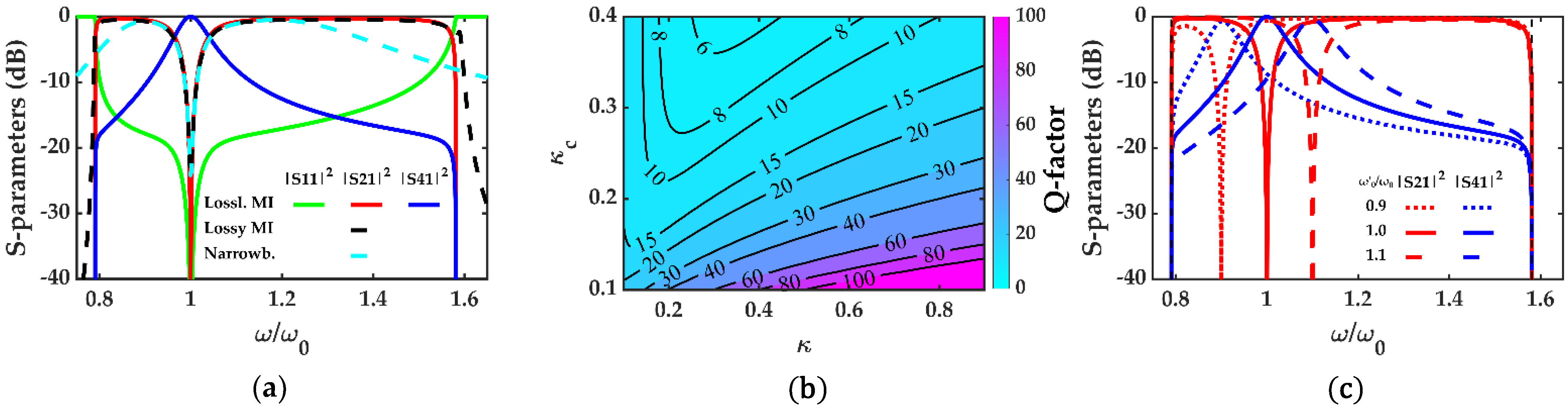
3.1. Single-Notch Filter

The overall design was as shown in Figure 2a; however, resistive terminations were used, and ports were floated using paired capacitors. To allow frequency tuneability, all capacitors included varicaps. To confine magnetic fields and ensure nearest-neighbour coupling, all inductors used low-loss ferrimagnetic toroidal cores with inner and outer diameters of 13.2 and 21 mm (Fair-Rite 5967000601, based on “67” Ni–Zn ferrite material with cutoff at 50 MHz). The initial relative permeability was ≈40, implying that the magnetic flux was almost completely contained in the core. Two windings (with inductances $L_C$ and $L_T$, such that $L_C+L_T=L$) were used for the waveguide elements, and three (with inductances $L_C$, $L_C$, and $L_S$, such that $2L_C+L_S=L$) for the coupling resonators. Adjacent windings were reversed to obtain negative coupling coefficients. A method was used to allow the tuning of mutual inductance using components constructed by 3D printing with a polycarbonate filament. Figure 6a shows this mechanism, allowing control over the relative position of two copper windings. The coupling coefficient was a nonlinear function of the winding separation with minimum separation yielding maximum coupling.

Figure 6b shows a photograph of the completed filter constructed as a copper-clad printed circuit board using low-loss mica capacitors. Mechanical tuning was provided for all mutual inductances. The value of $M$ needed for impedance matching to a $50\mathsf{\Omega }$ load at resonance was first identified. Inductors $L_s$ were then chosen to equalise the self-inductance of all resonators, and capacitances were tuned to achieve resonance at 13.56 MHz.

Table 1. Experimental parameter values.

Parameter	Value	Range of Adjustment
$L_T$	1.16 μH	N/A (not applicable)
$L_c$	460 nH	N/A
$L_s$	710 nH	N/A
$\kappa$	0.725	0.51–0.92
${\kappa }_c$	0.28	0.19–0.34
${\omega }_0$	13.56 MHz	DC to 50 MHz
$Q$	200 ± 10%	N/A

shows the values of the most important parameters after tuning.

Four-port scattering parameters were measured using an electronic network analyser (Agilent E5061B). To begin with, $\lambda$ was set to unity so that responses were independent of the port used as input. Figure 7a compares the frequency dependence of S-parameters with the predictions of the theoretical model for ${\kappa }_c=0.28$. Excellent agreement with experimental results can be seen. Larger values of $\mu$ were investigated and found to reduce losses and increase the passband of the bandpass channel and the notch depth.

3.2. Single-Notch Filter with Infinite Rejection

Stopband rejection can be greatly improved by fine-tuning $\lambda$ according to Equation (21). For parameters in Table 1, the value of $\lambda$ required for infinite rejection is 0.79, well within range for the coupling tuning mechanism. Figure 7b compares the simulated and measured scattering parameters obtained in this case. A performance improvement of over 50 dB is achieved compared with that in Figure 7a, with 70 dB rejection at port 2. This improvement is at the expense of reduced isolation of port 3 with a minimum attenuation of 18 dB at resonance between ports 1 and 3. However, losses in $S_{21}$are still extremely low.

3.3. Double-Notch Filters

A two-notch directional filter with parameter values shown in Table 1 was implemented in the same way by increasing the number of coupling resonators in each vertical branch from one to two. The magnitude of ${\kappa }_c$ determines the frequency locations of the notches in $S_{21}$ according to Equation (25). However, smaller values of ${\kappa }_c$ also increase propagation losses through the coupling resonators, reducing notch depth and increasing losses in the bandpass channel. Figure 8a compares theoretical and experimental results for ${\kappa }_c=0.3$. Agreement between simulation and experimental results is again excellent. Attenuation in $S_{21}$ is the same as for the single-notch filter, implying that two signals can be extracted simultaneously without hindering performance.

3.4. Double-Notch Filter with Improved Rejection

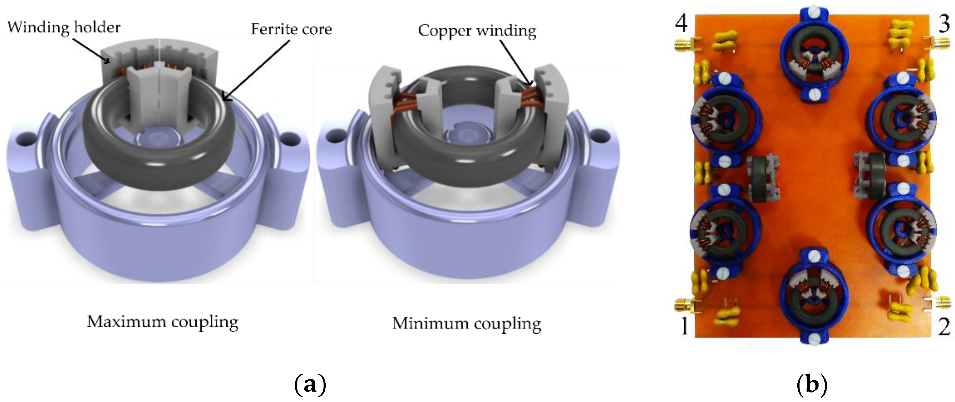
Although infinite rejection appears impossible in multinotch filters, rejection can be improved by adjusting $\lambda$. Figure 8b compares theoretical and measured S-parameters for a two-notch filter with ${\kappa }_c=0.3$ with $\lambda$ chosen to equalise rejection at the two notches. A significant performance improvement in a rejection of over 15 dB is obtained, once again at the expense of port 3 isolation. As regards single-notch filters, lower values of $\lambda$ are needed for higher values of $\mu$. Low insertion loss is observed around the resonance frequency but increases elsewhere as matching between the guides and load deteriorates.

3.5. Applications

Toroid transformers based on soft ferrites allow magnetoinductive designs to be realised with low non-nearest-neighbour coupling. However, core materials must have low loss and high linearity. Some applications also require high power handling. In HF RFID, a modulated AC magnetic field delivers power and data to tags, which couple to the field using inductive loops. For the ISO/IEC 14443 type A standard, the carrier frequency is $f_c=13.56 \mathrm{MHz}$, while tags use an internally generated subcarrier at $f_m=\frac{f_c}{16}$ to return data, generating sideband spectra with central frequencies, $f_c\pm f_m$. Since the carrier power can be orders of magnitude greater than that of the sidebands, receiver protection is required. The single-notch filter presented here can be integrated into existing MI systems via direct connection to the waveguides, has high rejection at resonance, and may be used to transfer residual carrier to a load. However, the filter must be effective at the representative carrier powers, despite potential nonlinearities introduced by ferrite cores. To emulate generic HF RFID signals, we modulated a high-power carrier at $f_c$ using a simple cosine message waveform at $f_m$. The waveform of the input signal $s\left(t\right)$ is:

$$s\left(t\right)=[A_c+A_m\cos \left(2\pi f_{m}t\right)]\cos \left(2\pi f_{c}t\right).$$

(26)

Here $A_c$ and $A_m$ are the carrier and message amplitudes. The signal was derived from a first signal generator (Agilent E4433B) modulated by a second signal modulator (Agilent N5181A) with amplification by a 27 dB power amplifier (Minicircuits ZFDWHA-1–20+). $A_c$ was adjusted to deliver a carrier power, $P_c$, into a 50 $\mathsf{\Omega }$load, while the modulation index $A_m/A_c$ was chosen to generate typically small sidebands. Detection was performed using a digital storage oscilloscope (Keysight InfiniiVision DSOX3024T, Santa Rosa, CA, USA) using a 30 dB attenuator for unfiltered signals. Figure 9a shows the power spectral density (PSD) of the signal input to port 1 of the single-notch filter for $P_c=1 W$. Amplifier nonlinearities have resulted in minor harmonics of the AM spectrum, which have been partially suppressed at high frequencies with a low-pass filter. Figure 9b shows the PSD at port 2, the stopband channel. The output shows a carrier attenuation of 73 dB and a sideband attenuation of 1.2 dB, implying an output signal with almost intact message and negligible carrier. No significant additional harmonics are introduced. Figure 9c shows the attenuation of the two sidebands and the carrier over a power range between 0.1 and 1 W. Attenuation is almost independent of $P_c$, implying effective power handling despite the use of ferrites.

3.6. Frequency Scaling

The potential for scaling to higher frequencies is largely determined by ferrite performance.

Table 2. Properties of a selection of ferrite materials and toroids.

Manufacturer	Model	OD (mm)	ID (mm)	Height (mm)	Initial μi	Fmax (MHz)	TC °C	Material	Loss Factor
Ferroxcube	-	-	-	-	125	20	>350	4C65	130 @ 10 MHz
Fair-Rite	5961001801	22.10	13.70	06.35	125	25	>300	61	10 @ 10 MHz
Ferroxcube	-	-	-	-	25	100	>400	4E2	-
Fair-Rite	5968001801	22.10	13.70	6.35	16	150	>500	68	300 @ 100 MHz
National Magnetics	-	-	-	-	7.5	400	>320	M5	<3500 @ 100 MHz

shows performance parameters for low-cost NiZn soft ceramic ferrite materials and toroids designed for RF applications, such as EMI suppressors (upper group) and broadband transformers and baluns (lower), including their initial relative permeability ${\mu }_i$, Curie temperature T_C, and loss factor. The main difference between groups is the maximum usable frequency F_max. Following Snoek’s limit [52], ${\mu }_i$falls as F_max is raised. High-frequency performance is therefore accompanied by a reduction in magnetic field confinement and an increase in loss. Small toroids may be used to minimise the volume of magnetic material. However, careful design will be required to optimise performance, power handling will be reduced, and automated coil winding may be required for construction [53]. Despite this, the data suggest that response may be extended to the low UHF band. Above this, air-cored inductors may be used, but non-nearest-neighbour coupling and radiation will inevitably complicate the design and reduce performance.

3.7. Future Work

MI directional filters can also be designed for use at UHF. Potential research could concentrate on counteracting ferrite losses or, alternatively, minimising non-nearest-neighbour coupling and radiation in open-loop designs. Furthermore, the device wave operating principles can be extended to other metamaterial types, such as elastic or acoustic [54]. In particular, it has already been shown by us that MEMS could be used to generate high-performance two-port notch and comb filters [55]. Once again, wave analysis was used to simplify the coupled dynamical equations. Extension to multiport devices can be a fitting research target. Higher performance is expected due to inherently higher Q-factors of MEMS resonators.

4. Conclusions

New configurations of a magnetoinductive device with directional filter properties have been introduced based purely on magnetically coupled LC resonators. Design rules have been established, and methods for calculating scattering parameters when filters are used in MI systems (which have complex, frequency-dependent impedance) or conventional systems (with real impedance) have been clarified. The circuit equations have been simplified and solved using wave analysis. Analytic expressions have been developed for S-parameters and bandwidth, a simple method for introducing tuneability has been proposed, and extensions to allow infinite rejection at a chosen frequency or multiple stopbands with high rejection have been described.

Device construction and operation have been verified at HF. Ceramic ferrite cores have been used to ensure nearest-neighbour coupling in a compact layout, and simple mechanical methods of tuning resonant frequency and coupling (essential in blocker applications) have been proposed and demonstrated. Experimental results for tuneable filters, filters with infinite rejection, and filters with multiple bandstop frequencies have all been shown to agree with theoretical models. Power handing capability sufficient for blocker applications in HF RFID has been demonstrated, with little harmonic generation due to ferrite nonlinearity. Further development will involve direct connection to a magnetoinductive antenna, and this work is in progress.

References

1. Cohn, S.; Coale, F. Directional Channel-Separation Filters. Proc. IRE 1956, 44, 1018–1024. [Google Scholar] [CrossRef]
2. Coale, F.S. A Traveling-Wave Directional Filter. IRE Trans. Micr. Theory Tech. 1956, 4, 256–260. [Google Scholar] [CrossRef]
3. Walker, J.L.B. Exact and Approximate Synthesis of TEM-Mode Transmission-Type Directional Filters. IEEE Trans. Micr. Theory Tech. 1978, 26, 186–192. [Google Scholar] [CrossRef]
4. Matthaei, G.L.; Young, L.; Jones, E.M. Design of Microwave Filters, Impedance-Matching Networks, and Coupling Structures; McGraw-Hill: New York, NY, USA, 1963; Chapter 14. [Google Scholar]
5. Coale, F.S. Applications of Directional Filters for Multiplexing Systems. IEEE Trans. Micr. Theory Tech. 1958, 6, 450–453. [Google Scholar] [CrossRef]
6. Wing, O. Cascade Directional Filter. IEEE Trans. Micr. Theory Tech. 1959, 7, 197–201. [Google Scholar] [CrossRef]
7. Cameron, R.; Yu, M. Design of manifold-coupled multiplexers. IEEE Microw. Mag. 2007, 8, 46–59. [Google Scholar] [CrossRef]
8. Tuttle, L.P.; Wanselow, R.D. Practical Design of Strip-Transmission-Line Half-Wavelength Resonator Directional Filters. IEEE Trans. Microw. Theory Tech. 1959, 7, 168–173. [Google Scholar] [CrossRef]
9. Moore, B.D.; Cogdell, J.R. A Millimeter-Wave Directional Filter Cavity. IEEE Trans. Microw. Theory Tech. 1976, 24, 843–847. [Google Scholar] [CrossRef]
10. Uysal, S. Microstrip loop directional filter. Electron. Lett. 1997, 33, 475. [Google Scholar] [CrossRef]
11. Rosloniec, S.; Habib, T. Novel microstrip-line directional filters. IEEE Trans. Microw. Theory Tech. 1997, 45, 1633–1637. [Google Scholar] [CrossRef]
12. Cheng, Y.; Hong, W.; Wu, K. Half Mode Substrate Integrated Waveguide (HMSIW) Directional Filter. IEEE Microw. Wireless Comp. Lett. 2007, 17, 504–506. [Google Scholar] [CrossRef]
13. Kim, J.P. Improved Design of Single-Section and Cascaded Planar Directional Filters. IEEE Trans. Microw. Theory Tech. 2011, 59, 2206–2213. [Google Scholar] [CrossRef]
14. Zhang, Y.; Shi, S.; Martin, R.D.; Prather, D.W. Slot-Coupled Directional Filters in Multilayer LCP Substrates at 95 GHz. IEEE Trans. Microw. Theory Tech. 2017, 65, 476–483. [Google Scholar] [CrossRef]
15. Zhang, Y.-B.; Chen, B.; Ran, C.-Z. An X-band single-layer waveguide directional filter with compact size and low insertion loss. IEICE Electron. Express 2018, 15, 20180826. [Google Scholar] [CrossRef]
16. Stone, A.M.; Lawson, J.L. Infinite-Rejection Filters. J. Appl. Phys. 1947, 18, 691–703. [Google Scholar] [CrossRef]
17. Parthasarathy, D.; Harjani, R. Novel integratable notch filter implementation for 100 dB image rejection. In Proceedings of the 2003 International Symposium on Circuits and Systems, ISCAS’03, Bangkok, Thailand, 25–28 May 2003. [Google Scholar]
18. Jachowski, D.R. Passive enhancement of resonator Q in microwave notch filters. In Proceedings of the 2004 IEEE MTT-S International Microwave Symposium Digest (IEEE Cat. No.04CH37535), Fort Worth, TX, USA, 6–11 June 2004. [Google Scholar]
19. Jachowski, D.R. Compact, frequency-agile, absorptive bandstop filters. In Proceedings of the IEEE MTT-S International Microwave Symposium Digest, 2005, Long Beach, CA, USA, 17 June 2005. [Google Scholar]
20. Ghaffari, A.; Klumperink, E.A.M.; Nauta, B. Tunable N-Path Notch Filters for Blocker Suppression: Modeling and Verification. IEEE J. Solid-State Circuits 2013, 48, 1370–1382. [Google Scholar] [CrossRef]
21. Lababidi, R.; Le Roy, M.; Le Jeune, D.; Perennec, A.; Vauche, R.; Bourdel, S.; Gaubert, J. Compact highly selective passive notch filter for 3.1–5 GHz UWB receiver system. In Proceedings of the 2015 IEEE International Conference on Electronics, Circuits, and Systems (ICECS), Cairo, Egypt, 6 December 2015. [Google Scholar]
22. Morgan, M.A.; Boyd, T.A. Theoretical and Experimental Study of a New Class of Reflectionless Filter. IEEE Trans. Microw. Theory Tech. 2011, 59, 1214–1221. [Google Scholar] [CrossRef]
23. Morgan, M.A.; Boyd, T.A. Reflectionless Filter Structures. IEEE Trans. Microw. Theory Tech. 2015, 63, 1263–1271. [Google Scholar] [CrossRef] [Green Version]
24. Standley, R.D. A Time-Delay Equalizer Using Directional Filter Cascades. IEEE Trans. Microw Theory Tech. 1971, 19, 497–498. [Google Scholar] [CrossRef]
25. Erickson, N.R. A Directional Filter Diplexer Using Optical Techniques for Millimeter to Submillimeter Wavelengths. IEEE Trans. Microw. Theory Tech. 1977, 25, 865–866. [Google Scholar] [CrossRef]
26. Hunter, I.; Musonda, E.; Parry, R.; Guess, M.; Meng, M. Transversal directional filters for channel combining. In Proceedings of the 2013 IEEE MTT-S International Microwave Symposium Digest (MTT), Seattle, WA, USA, 2–7 June 2013. [Google Scholar]
27. Sorocki, J.; Piekarz, I.; Gruszczynski, S.; Wincza, K. Miniaturized directional filter multiplexer for band separation in UWB antenna systems. In Proceedings of the 2015 International Symposium on Antennas and Propagation (ISAP), Hobart, Australia, 9–12 November 2015; pp. 1–4. [Google Scholar]
28. Wincza, K.; Gruszczynski, S. Frequency-Selective Feeding Network Based on Directional Filter for Constant-Beamwidth Scalable Antenna Arrays. IEEE Trans. Antennas Propag. 2017, 65, 4346–4350. [Google Scholar] [CrossRef]
29. Sun, J.S.; Lobato-Morales, H.; Choi, J.H.; Corona-Chavez, A.; Itoh, T. Multistage Directional Filter Based on Band-Reject Filter with Isolation Improvement Using Composite Right-/Left-Handed Transmission Lines. IEEE Trans. Microw. Theory Tech. 2012, 60, 3950–3958. [Google Scholar] [CrossRef]
30. Beruete, M.; Falcone, F.; Freire, M.J.; Marqués, R.; Baena, J.D. Electroinductive waves in chains of complementary metamaterial elements. Appl. Phys. Lett. 2006, 88, 083503. [Google Scholar] [CrossRef] [Green Version]
31. Liu, N.; Kaiser, S.; Giessen, H. Magnetoinductive and Electroinductive Coupling in Plasmonic Metamaterial Molecules. Adv. Mater. 2008, 20, 4521–4525. [Google Scholar] [CrossRef]
32. Navarro-Cia, M.; Carrasco, J.M.; Beruete, M.; Falcone, F.J. Ultra-wideband metamaterial filter based on electro-inductive wave coupling between microstrips. PIER Lett. 2009, 12, 141–150. [Google Scholar] [CrossRef] [Green Version]
33. Gil, M.; Velez, P.; Aznar-Ballesta, F.; Munoz-Enano, J.; Martin, F. Differential Sensor Based on Electroinductive Wave Transmission Lines for Dielectric Constant Measurements and Defect Detection. IEEE Trans. Antennas Propag. 2020, 68, 1876–1886. [Google Scholar] [CrossRef]
34. Shamonina, E.; Kalinin, V.A.; Ringhofer, K.H.; Solymar, L. Magneto-inductive waveguide. Electron. Lett. 2002, 38, 371. [Google Scholar] [CrossRef]
35. Shadrivov, I.V.; Reznik, A.N.; Kivshar, Y.S. Magnetoinductive waves in arrays of split-ring resonators. Physica B 2007, 394, 180–183. [Google Scholar] [CrossRef]
36. Stevens, C.J.; Chan, C.W.T.; Stamatis, K.; Edwards, D.J. Magnetic Metamaterials as 1-D Data Transfer Channels: An Application for Magneto-Inductive Waves. IEEE Trans. Microw. Theory Tech. 2010, 58, 1248–1256. [Google Scholar] [CrossRef]
37. Sun, Z.; Akyildiz, I.F. Magnetic Induction Communications for Wireless Underground Sensor Networks. IEEE Trans. Antennas Propag. 2010, 58, 2426–2435. [Google Scholar] [CrossRef] [Green Version]
38. Gulbahar, B.; Akan, O.B. A Communication Theoretical Modeling and Analysis of Underwater Magneto-Inductive Wireless Channels. IEEE Trans. Wireless Comms 2012, 11, 3326–3334. [Google Scholar] [CrossRef]
39. Zhong, W.; Lee, C.K.; Hui, S.Y.R. General Analysis on the Use of Tesla’s Resonators in Domino Forms for Wireless Power Transfer. IEEE Trans. Indust. Electron. 2013, 60, 261–270. [Google Scholar] [CrossRef] [Green Version]
40. Agbinya, J.I. A magneto-inductive link budget for wireless power transfer and inductive communication systems. PIER C 2013, 37, 15–28. [Google Scholar] [CrossRef] [Green Version]
41. Stevens, C.J. A magneto-inductive wave wireless power transfer device. Wireless Power Transf. 2015, 2, 51–59. [Google Scholar] [CrossRef] [Green Version]
42. Freire, M.J.; Marqués, R. Planar magnetoinductive lens for three-dimensional subwavelength imaging. Appl. Phys. Lett. 2005, 86, 182505. [Google Scholar] [CrossRef]
43. Syms, R.R.A.; Young, I.R.; Ahmad, M.M.; Rea, M. Magnetic resonance imaging using linear magneto-inductive waveguides. J. Appl. Phys. 2012, 112, 114911. [Google Scholar] [CrossRef] [Green Version]
44. Floume, T. Magneto-inductive conductivity sensor. Metamaterials 2011, 5, 206–217. [Google Scholar] [CrossRef]
45. Yan, J.; Stevens, C.J.; Shamonina, E. A Metamaterial Position Sensor Based on Magnetoinductive Waves. IEEE Open J. Antennas Propag. 2021, 2, 259–268. [Google Scholar] [CrossRef]
46. Syms, R.R.A.; Sydoruk, O.; Wiltshire, M.C.K. Magneto-Inductive HF RFID System. IEEE J. RFID 2021, 5, 148–153. [Google Scholar] [CrossRef]
47. Shamonina, E.; Solymar, L. Magneto-inductive waves supported by metamaterial elements: Components for a one-dimensional waveguide. J. Phys. D Appl. Phys. 2004, 37, 362–367. [Google Scholar] [CrossRef]
48. Syms, R.R.A.; Shamonina, E.; Solymar, L. Magneto-inductive waveguide devices. IEE Proc. Microw. Antennas Propag. 2006, 153, 111. [Google Scholar] [CrossRef] [Green Version]
49. Syms, R.R.A.; Solymar, L.; Young, I.R. Broadband coupling transducers for magneto-inductive cables. J. Phys. D Appl. Phys. 2010, 43, 285003. [Google Scholar] [CrossRef] [Green Version]
50. Kurokawa, K. Power Waves and the Scattering Matrix. IEEE Trans. Microw. Theory Tech. 1965, 13, 194–202. [Google Scholar] [CrossRef] [Green Version]
51. Voronov, A.; Sydoruk, O.; Syms, R.R.A. Power waves and scattering parameters in magneto-inductive systems. AIP Adv. 2021, 11, 045327. [Google Scholar] [CrossRef]
52. Snoek, J.L. Dispersion and absorption in magnetic ferrites at frequencies above one Mc/s. Physica 1948, 14, 207–217. [Google Scholar] [CrossRef]
53. Kazimierczuk, M. High-Frequency Magnetic Components; John Wiley & Sons: Chichester, UK, 2014. [Google Scholar] [CrossRef]
54. Wang, Y.; Wang, Y.; Wu, B.; Chen, W.; Wang, Y. (February 26, 2020). Tunable and active phononic crystals and metamaterials. ASME. Appl. Mech. Rev. 2020, 72, 040801. [Google Scholar] [CrossRef]
55. Bouchaala, A.; Syms, R.R.A. New architectures for micromechanical coupled beam array filters. Microsyst. Technol. 2021, 27, 3377–3387. [Google Scholar] [CrossRef]
Figure 1. Magnetoinductive (MI) waveguide: (a) equivalent circuit; (b) frequency dependence of k a and k a for κ = { ± 0.6 , ± 0.3 } and Q = 200 . Crosses show measured points for   κ = 0.3 .
Electronics 11 00845 g001
Figure 2. (a) MI directional filter equivalent circuit; (b) lumped element terminations: (1) magnetoinductive, (2) resistive, and (3) broadband resistive.
Electronics 11 00845 g002
Figure 3. MI directional filter performance for κ = 0.6 and κ c = 0.3 : (a) scattering parameters for lossless and lossy ( Q = 200 ) resonators with MI terminations (1) and real narrowband terminations (2); (b) variation of Q b p with κ and κ c for a lossless filter with MI terminations (1); (c) scattering parameters for lossless resonators with MI terminations (1) for ω 0 / ω 0 = 0.9 ,   1.0 ,   and   1.1 .
Electronics 11 00845 g003
Figure 4. (a) Variation of λ with μ for different unloaded resonator Q-factors with κ = 0.6 . (b) Frequency dependence of scattering parameters for infinite rejection filter with lossy MI and resistive narrowband terminations with κ = 0.6 , κ c = 0.3 , and   Q = 200 .
Electronics 11 00845 g004
Figure 5. (a) Multiple bandstop MI directional filter; (b) frequency dependence of S-parameters for multiple passband filter with lossless MI terminations (1) for κ = 0.6 , κ c = 0.3 ,   N = 2 , and N = 5 .
Electronics 11 00845 g005
Figure 6. MI directional filter: (a) mechanism for tuning of magnetic coupling (LH–maximum coupling; RH–minimum coupling); (b) complete PCB with labelled port numbers.
Electronics 11 00845 g006
Figure 7. Experimental (solid) and theoretical (dashed) frequency dependence of scattering parameters for MI filter with resistive narrowband terminations (2) with ω 0 = 13.56 MHz, Q = 200 , and Z 0 M = 50   Ω . (a) κ c = 0.28 and λ = 1 ; (b) infinite rejection with κ c = 0.25 and λ = 0.79.
Electronics 11 00845 g007
Figure 8. Experimental (solid) and theoretical (dashed) frequency dependence of S-parameters for double passband MI filter with resistive narrowband terminations with ω 0 = 13.56 MHz, Q = 180 , Z 0 M = 50   Ω , and κ c = 0.3 . (a) No improved rejection; (b) improved rejection.
Electronics 11 00845 g008
Figure 9. Power spectral densities of (a) input signal to port 1 of MI single-notch directional filter; (b) output signal at port 2 normalised by the input carrier power P c . Dashed lines: filter bandwidth; red: harmonics at multiples of carrier frequencies; green: harmonics at message sidebands. (c) Attenuation of sidebands and carrier.
Electronics 11 00845 g009